Essays in inflation and monetary dynamics in developing countries

(1)

Dissertations, Theses, and Student Research

from the College of Business Business, College of

Summer 8-10-2012

Essays in inflation and monetary dynamics in developing

countries

Simon K. Harvey

University of Nebraska-Lincoln

Follow this and additional works at: https://digitalcommons.unl.edu/businessdiss

Part of the Business Commons, Econometrics Commons, and the International Economics Commons Harvey, Simon K., "Essays in inflation and monetary dynamics in developing countries" (2012).

Dissertations, Theses, and Student Research from the College of Business. 30. https://digitalcommons.unl.edu/businessdiss/30

This Article is brought to you for free and open access by the Business, College of at DigitalCommons@University of Nebraska - Lincoln. It has been accepted for inclusion in Dissertations, Theses, and Student Research from the College of Business by an authorized administrator of DigitalCommons@University of Nebraska - Lincoln.

(2)

By% % % % Simon%Kwadzogah%Harvey% % % % A%DISSERTATION% % Presented%to%the%Faculty%of% The%Graduate%College%at%the%University%of%Nebraska% In%Partial%Fulfillment%of%Requirements% For%the%Degree%of%Doctor%of%Philosophy% % % Major:%Economics% % Under%the%Supervision%of%Professor%Matthew%J.%Cushing% % % % Lincoln,%Nebraska% August%2012%

(3)

Simon%Kwadzogah%Harvey,%PhD% University%of%Nebraska%2012% Advisor:%Matthew%J.%Cushing%

This% dissertation% is% consists% of% three% essays.% In% the% first% essay,% I% analyze% how% the% information%contained%in%the%disaggregate%components%of%aggregate%inflation%helps% improve%the%forecasts%of%the%aggregate%series%using%inflation%data%from%Ghana.%Direct% univariate% forecasting% of% the% aggregate% inflation% data% by% an% autoregressive% (AR)% model%is%used%as%the%benchmark%with%which%all%autoregressive%(AR),%moving%average% (MA)% and% vector% autoregressive% (VAR)% models% of% the% disaggregates% are% compared.% The%results%show%that%directly%forecasting%the%aggregate%series%from%the%benchmark% model% is% generally% superior% to% aggregating% forecasts% from% the% disaggregate% components.% Additionally,% including% information% from% the% disaggregates% in% the% aggregate%model%rather%than%aggregating%forecasts%from%the%disaggregates%performs% best% in% all% forecast% horizons% when% appropriate% disaggregates% are% used.% The% implication%of%these%results%is%that%better%inflation%forecasts%for%Ghana%are%produce% by% using% information% from% relevant% disaggregates% in% the% aggregate% model% rather% than% direct% forecasts% of% the% aggregate% or% aggregating% forecasts% from% the% disaggregates.%

In% the% second% essay,% I% use% a% structural% vector% autoregression% (SVAR)% to% model% inflation%so%as%to%identify%the%relative%importance%of%shocks%to%real%output%growth,% monetary% growth% and% exchange% rate% depreciation% in% inflation% dynamics% in% Ghana.% The% results% show% that% neither% monetary% growth% alone% nor% structural% factors% alone%

(4)

monetary% growth% in% the% inflation% dynamics.% There% is% a% fairly% strong% feedback% between% inflation% and% exchange% rate% depreciation% both% of% which% have% weak% relationship%with%monetary%growth.%These%suggest%that%policies%that%boost%domestic% supply% and% therefore% reduce% import% demand% will% be% more% potent% than% direct% monetary%management%to%curb%inflation%in%Ghana.%

Finally,% in% the% third% essay,% I% the% test% whether% the% West% African% Monetary% Zone% (WAMZ)%is%a%common%currency%area%by%using%a%vector%autoregressive%model%to%study% the%variance%decomposition,%impulse%responses%of%key%economic%variables%and%linear% dependence% of% the% underlying% structural% shocks% of% the% countries% in% the% zone.% The% variance% decomposition% shows% that% the% zone% a% whole% does% not% have% common% sources%of%shock,%which%is%expected%because%of%the%diverse%economic%structures%of% these% countries.% The% correlation% of% the% structural% shocks% also% shows% that% these% countries%respond%asymmetrically%to%common%supply,%demand%and%monetary%shocks% and%will%therefore%respond%differently%to%a%common%monetary%policy.%It%is%therefore% not%in%the%interest%of%the%individual%countries%to%go%into%a%monetary%union%now%or%in% the%near%future%unless%the%economies%of%these%countries%converge%further.%

(5)

DEDICATION

(6)

ACKNOWLEDGMENTS

I sincerely acknowledge the contribution of Professor Matthew Cushing to my academic carrier. From time of application for the program through coursework and dissertation to graduation, Professor Cushing has always been ready and willing to help me succeed. I truly appreciate his mentoring throughout the PhD program especially during the dissertation period when he became the chair of my dissertation committee. He did not “spare the rod to spoil the child”. Beyond academics, Professor Cushing has been very much interested in the welfare of my family in times of difficulties. I am, and will forever be grateful for the support. I cannot thank him enough.

I appreciate the timely response of the members of my dissertation committee; Professor James Schmidt, Professor Eric Thompson and Professor John Geppert. I owe my timely completion of the program to them and to McConnell Fellowship for providing with stipend for ten months during the period of my dissertation writing to enable me concentrate on research. Also, Office of Research, Innovation and Development (ORID) of University of Ghana provided me with a grant to support my research and University of Ghana Business School supplemented my living expenses.

Mr. and Mrs. Roger and Julie Sand have been very good my wife and I throughout our stay in the United States. Inviting us to their home on every important occasion to meet family members and taking us to their cabin to cruise and learn more of American culture were pleasurable moments that we cherish so much and cannot forget. I thank them so much for their generosity. I thank Bernard Walley for his friendship and willingness to talk with me on the phone for hours to discuss both academic and personal issues. I also thank Andy Boateng and the family for their friendship. Finally, the greatest of all the thanks go to my wife Vickita, to whom I dedicate this

(7)

work, for all the sacrifices she has made during the course of my PhD program.

While all the above acknowledgements are for people I know and see often, I would like to acknowledge that without the grace of God Almighty, the unseen, who gives good health and life, nothing would have gone right.

(8)

LIST OF TABLES

Table 2.1: Descriptive statistics ... 21!

Table 2.2: Unit root tests of the variables in the data (ADF p-values) ... 23!

Table 2.3: Weights for aggregating forecasts ... 24!

Table 2.4: Pairwise Granger causality between the aggregate and the disaggregate series ... 26!

Table 2.5: Root Mean Square Forecast Error (RMSE) for year-on-year inflation ... 29!

Table 3.1: Augmented Dickey-Fuller tests ... 49!

Table 3.2: Variance decomposition of real output growth ... 50!

Table 3.3: Variance decomposition of inflation ... 50!

Table 3.4: Variance decomposition of exchange rate ... 51!

Table 3.5: Variance decomposition of money supply (M+) ... 51!

Table 4.1: Performance of WAMZ countries on primary convergence criteria ... 70!

Table 4.2: Structure and real GDP growth of WAMZ countries ... 72!

Table 4.3: Variance decomposition of the variables in the model ... 84!

Table 4.4: Relationship between supply shocks ... 93!

Table 4.5: Relationship between demand shocks ... 95!

Table 4.6: Relationship between monetary shocks ... 97! !

(12)

LIST OF FIGURES

Figure 2.1: Graphs of the level of the series in the dataset ... 22!

Figure 3.1: Year-on-year monthly Inflation in Ghana ... 38!

Figure 3.2: Year-on-year monthly monetary (M2+) growth in Ghana ... 40!

Figure 3.3: Graphs of the variables in the models ... 48!

Figure 4.1: Impulse response for Gambia ... 86!

Figure 4.2: Impulse response for Ghana ... 87!

Figure 4.3: Impulse response for Guinea ... 88!

Figure 4.4: Impulse response for Nigeria ... 89!

(13)

1 CHAPTER 1: INTRODUCTION 1.1 Background

This study consists of three papers: “Does using disaggregate components help in producing better forecasts for aggregate inflation?”, “Separating monetary and structural causes of inflation” and “Is West African Monetary Zone (WAMZ) a common currency area?” The motivation for the first paper stems from the fact that the private sector, governmental and international institutions as well as central banks use forecasts of macroeconomic aggregates, especially inflation in their decision-making. This makes inflation one of the main economic aggregates forecast by central banks around the world, because of their responsibilities in maintaining stable prices. Additionally, other macroeconomic policies depend on inflation forecasts.

Prior literature on inflation forecasting has employed univariate aggregate series. However, the question is whether inflation forecasts can be improved by aggregating forecasts from subcomponents. In an attempt to answer this question, studies have developed on sectoral disaggregation of inflation series (Aron and Mueller(2008), de Dois Tena et al.(2010) and Hendry and Hubrisch(2005)). While the theoretical literature is clear on the conditions under which forecasting aggregate series, empirical results have not reached any consensus on whether disaggregation by sectors improves forecast of the aggregate series. Also, the concentration of the studies on the heterogeneity across product categories and the neglect of spatial heterogeneity perhaps are based on the implicit assumption of the Law of One Price, which assumes that the product markets are efficient. While these assumptions may hold for the developed economies, spatial heterogeneity in price developments may be significant in developing and emerging

(14)

market economies where information is asymmetric due to poor transportation and telecommunication infrastructure. This paper fills the gap by looking at the subcomponents in other dimensions such as the regional and rural-urban series.

The second paper is motivated by the fact that there are two schools of thought on what explains inflation; monetary growth or structural factors. The monetarist believes that money is all that matters in explaining inflation. Their argument is based on the link between monetary growth and domestic prices, which is rooted in the traditional quantity theory of money, which forms the basis of the monetarist statement that “inflation is always and everywhere a monetary phenomenon”. The structuralists, on the other hand, believe that structural and institutional factors play a more prominent role in inflation dynamics. The structuralists’ argue that inelastic food supply, infrastructural problems posing problems for distribution of output, lack of financial resources and low export receipts leading to foreign exchange shortages in less developing countries put pressure on domestic prices (London(1989)). The nominal exchange rate pass-through to domestic price inflation depends on how the changes in the exchange rates are passed through to import prices and therefore to domestic consumer prices (Mishkin(2008)). These structural factors can be categorized into supply, demand, monetary and direct price shocks to inflation. In the case of Ghana, it is not known what actually explains the inflationary dynamics, which is what this paper sets out to provide.

Finally, the proposal for the introduction of a single currency within the West African Monetary Zone (WAMZ) and the fact that there have been unsuccessful attempts at introducing it inspires the third paper to ascertain if the right economic conditions for a successful introduction and maintenance of a single currency exits in the zone. It has been initially proposed to implement the monetary integration process in in Economic community of West African States (ECOWAS)

(15)

as a whole but due to the complexities of the process, it was later change to a two-stage implementation where a second monetary zone, the West African Monetary Zone (WAMZ) for the Anglophone West Africa is formed, which will later merge with the existing zone, the West Africa Economic and Monetary Union (WAEMU) for the Francophone West Africa. Since the introduction of the proposed single currency is in two stages analyzing the convergence of non-CFA countries alone will draw a better picture of what is needed now by ECOWAS.

1.2 Objectives of the study

The study aims at contributing to the literature by analyzing inflation and monetary dynamics of emerging economies. In the light of this, three distinct research papers will be produced.

The first research paper extends the previous studies by considering disaggregation across regions, rural – urban as well as product groups. Also, the study investigates whether including disaggregate information in the aggregate model for inflation can improve the forecasts of the aggregate series.

The second paper identifies the extent to which shocks to real output growth, monetary growth and exchange rate depreciation explain inflation dynamics in Ghana. Specifically, this paper explores two objectives. First, it identifies the relative importance of output supply shocks, money supply changes and exchange rate changes in inflation dynamics by analyzing the variance decomposition of the forecast error variance of inflation a Structural Vector Autoregression (SVAR). Secondly, the paper analyzes how shocks to changes in money supply and exchange rates transmit through to price developments and how fast these shocks dissipate.

(16)

The third research paper tests whether the economies of the ECOWAS member countries are exposed to similar sources of shock. This will be done by studying the impulse-response functions of the countries in a Structured Vector Autoregression (SVAR) to determine if it takes similar times for common shocks to dissipate across the region. The paper will also test the linear dependence of these shocks using Geweke(1982) measure of linear dependence.

1.3 Methodologies

Each of these research papers employs estimation strategy that is unique and addresses a specific research question. The overview of these methodologies a given below.

1.3.1 Does(using(disaggregate(components(help(in(producing(better(forecasts(for(

aggregate(inflation?(

A benchmark model of the aggregate series with which all the other models are compared is the simple autoregressive (AR) model. Granger-causality tests are done to determine which of the disaggregate series contain more information in forecasting the aggregate series. The individual components of the aggregate inflation series are modeled jointly in an unrestricted Vector Autoregressions (VAR) and the forecasts from these models are aggregated and compared with the benchmark forecasts from the aggregate inflation series using on the Root Mean Square Error (RMSE) of the forecasts. Also, the disaggregate components are included in vector autoregressive (VAR) with the aggregate series and aggregate series forecast from these VARs and compared. The optimal lag selection for all the models are based on Akaike Information Criterion (AIC).

(17)

1.3.2 Separating(monetary(and(structural(causes(of(inflation.(

The approach to modeling inflation in this paper is to identify the variables that are found to explain inflation dynamics in Africa, from the literature, and analyze these variables in a Structural Vector Autoregression by imposing appropriate economic theory on their dynamic relationship. Monetary growth and exchange rate depreciation have a significant positive relationship with inflation in African countries (Canetti and Greene(1991)), and the structuralist argument also maintained that real GDP growth explains the inflationary process in developing countries. So in modeling monetary policy transmissions to inflation in Ghana, four endogenous variables, real GDP, inflation, nominal exchange rate of the Ghanaian cedi against the US dollar and monetary growth are considered in a Structural Vector Autoregression (SVAR). The identification of the structural shocks from the SVAR are based on Blachard and Quah(1989).

1.3.3 Is(West(African(Monetary(Zone((WAMZ)(a(common(currency(area?(

The method of identifying shock asymmetry across the WAMZ derives from the trivariate Structural Vector Autoregression (SVAR) used by Clarida and Gali(1994) and Kempa(2002) to recover demand, supply and monetary shocks to real economic activity, real exchange rate changes and price level changes. The three endogenous variables that will be considered are a measure of growth of economic activity of a country relative to the US, change in bilateral real exchange rates between each country’s currency and the US dollar and change in price level of each country relative to the US price level. The identification of the structural shocks from the SVAR is based on Gali(1992).

1.4 Data sources

The data on inflation rates are obtained from Ghana Statistical Service. The published series are monthly data categorized by the level 1 of United Nation’s Classification of Individual

(18)

Consumption by Purpose (CIOCOP) and by administrative regions of Ghana. The paper uses monthly data from January 2000 to December 2011.

Data on policy variables of the Banks of Ghana and other member countries of WAMZ are sourced from IMF’s International Financial Statistics (IFS). Data on trade that are used as a measure of economic activity are obtained from Direction of Trade Statistics, which is also published by the IMF. These data are validated by the data from reports of the central banks of the countries and individual country reports published by the West Africa Monetary Institute (WAMI). For the models on monetary policy and common currency issues, monthly data covering the period January 1982 to October 2011 are used. The start date is chosen based on the preliminary survey of the data that indicates that data is available for all the countries in the sub-region for that period.

1.5 Organization of the study

The dissertation is organized into five chapters. Chapter 1 covers the introduction to the dissertation while the succeeding three chapters cover each of the papers respectively. Chapter 5 draws overall conclusions from the results and provides policy implications emanating from the findings of the three core chapters.

(19)

References

Aron, J. and N. J. Mueller(2008). "Multi-Sector Inflation Forecasting - Quarterly Models for South Africa." CSAE, WPS/2008-27.

Blachard, O.J. and D Quah(1989). "The Dynamic Effects of Aggregate Demand and Supply Disturbances." American Economic Review, 79(4), pp. 655-673.

Canetti, E. and J. Greene(1991). "Monetary Growth and Exchange Rate Depreciation as Causes of Inflation in African Countries: An Empirical Analysis." IMF WORKING PAPER, International Monetary Fund, WP/91/67.

Clarida, R and J Gali(1994). "Sources of Real Exchange Rate Fluctuations: How Important Are Nominal Shocks?" Carnegie-Rochester Conference Series on Public Policy, 41, pp. 1-56.

de Dois Tena, J. ; A. Espasa and G. Pino(2010). "Forecasting Spanish Inflation Using Maximum Disaggregation Level by Sectors and Geographical Regions." International Regional Science Review, 33 (2), 181-204.

Gali, J(1992). "How Well Does the Is-Lm Model Fit the Postwar Us Data." The Quaterly Journal of Economics, 107(2), pp. 709 - 738.

Geweke, J.(1982). "Measurement of Linear Dependence and Feedback between Multiple Time Series." Journal of American Statistical Association, 77(378), pp. 304 - 313.

Hendry , D. F. and K. Hubrisch(2005). " Forecasting Aggregates with Disaggregates." Manuscript.

Kempa, B(2002). "Is Europe Converging to Optimality? On Dynamic Aspects of Optimum Currency Areas." Journal of Economic Studies, 29(2), pp. 109 - 120.

London, A.(1989). "Money, Inflation, and Adjustment Policy in Africa: Some Further Evidence." African Development Review, 1(1989), pp. 87-111.

Mishkin, F. S.(2008). "Exchange Rate Pass-through and Monetary Policy." Speech At the Norges Bank Conference on Monetary Policy, Oslo, Norway.

Vandaele, W.(1983). "Applied Time Series and Box-Jenkins Models." Academic Pres Inc., New York.

(20)

2 CHAPTER 2: DOES USING DISAGGREGATE COMPONENTS HELP IN PRODUCING BETTER FORECASTS FOR AGGREGATE INFLATION? 2.1 Introduction

Central banks all over the world are charged with the responsibility of maintaining low and stable prices in their countries. To achieve their goals, the central banks adopt monetary policy frameworks that they believe address local inflation problems. Many of these central banks adopt inflation targeting as their monetary policy framework, which makes accurate inflation forecasts indispensable. Apart from the use of inflation forecasts by central banks and other macroeconomic policy authorities, consumers, businesses, and other policy oriented institutions need inflation forecasts for planning purposes. Additionally, other macroeconomic policies depends, to a great extend, on inflation forecasts. The standard practice, as seen in the published data sets, is that inflation is calculated for sectors and other disaggregate components but forecasting in many cases has been performed using the aggregate series.

A recent question arising in the literature is whether aggregate inflation forecasts can be improved by using information from the subcomponents. In attempts to answer this question, literature has developed on the use of information from sectoral disaggregates of inflation series (see for example Aron and Mueller(2008), de Dois Tenaet al.(2010), and Hendry and Hubrisch(2005)). These studies, however, concentrate on disaggregation by product sectors. The concentration of the studies on product categories and the neglect of spatial categories like regions and rural – urban classifications perhaps are based on the implicit assumption of the Law of One Price, which assumes that product markets are efficient. While these assumptions may hold true for the developed economies, spatial heterogeneity in price developments may be

(21)

significant in developing and emerging market economies where information is asymmetric due to poor road and telecommunication infrastructure.

Although theoretical literature is clear on the conditions under which forecasting aggregate series from the sub-components will outperform the direct forecasting of the aggregate series, empirical studies have reached mixed conclusions. This study extends the previous studies by considering disaggregation across regions, rural – urban as well as product groups and applies the test to data from a developing economy, Ghana. Although previous studies have aggregated forecasts from the disaggregates, this study tests whether including the disaggregates in the aggregate model improves forecasts of the aggregate series. Also, the study investigates which form of disaggregation makes a more significant difference to the aggregate forecast and tests whether pooling forecast from both dimensions can make improve aggregate forecasts. Apart from using the rural – urban and regional forecasts to compare forecast improvements or otherwise of the series, forecasts of the components are important for regional and business planning.

The rest of the paper is structured as follows; section 2 is an overview of the existing literature on the subject. Section 3 discusses the methodologies used in the analysis of the data while section 4 discusses the empirical results. Section 5 states the conclusions and recommendations.

2.2 Literature review

The issue of whether micro models explain and/or forecast macro/aggregate series better started with Theil(1954) and expanded later by Grunfeld and Griliches(1960). Series of studies have been done after these pioneering works, which identify three alternatives to using the disaggregate components to improve on the direct forecasts of aggregate series. One approach is to model the subcomponents independently and aggregate the forecast from the independent

(22)

models based on a weighting scheme. A second approach is to model the subcomponents jointly in a vector autoregression (VAR) and the forecasts of the subcomponents from the VAR are aggregated into an aggregate forecast. A third approach is to use the disaggregate components in the aggregate model and forecast the aggregate directly.

Grunfeld and Griliches(1960) show, by comparing R!_{from OLS regression from aggregate} variable and composite R!_{calculated from}_R!_′s_{of OLS regressions of individual components,} that there is no gain in explaining an aggregate variable by aggregating the results of the components. A formal test for Grunfeld and Griliches(1960) procedure for discriminating between the composite model and the aggregate model stated in Pesaran et al.(1989) as choosing the micro models approach if the hypothesis H!:!e!′e! <e!′e! holds, where e!′e! is the

composite sum of square error computed from the micro models and e_!′e_! is the sum of square error from the aggregate model. Grunfeld and Griliches(1960) therefore conclude that if the data generating process at the micro level in not known, it is better to forecast the aggregate series directly. Building on this, Pesaranet al.(1989) note that Grunfeld and Griliches(1960) procedure suffers from finite sample bias and develops a choice criterion, and a test of perfect aggregation, for discriminating between aggregate and disaggregate models. Pesaranet al.(1989) test corrects for the finite sample bias and account for the contemporaneous correlation among the micro models. This test is further generalized by van Garderen et al.(2000) for application in non-linear models.

Pesaranet al.(1989)’s application of their tests to employment functions for the UK economy disaggregated by 40 industries and the manufacturing sector disaggregated by 23 industries find that the disaggregated model fits better than the aggregate model for the whole economy but not

(23)

for the manufacturing sector. They however interpret the performance of the aggregate model in the case of the manufacturing sector as a misspecification of the aggregate model.

Kohn(1982) and Lutkepohl(1984) consider the problem in time series forecasting setting and give a set of conditions under which a linear combination of the components of an aggregate series can forecast the aggregate series from its past. According to these studies, if x_! is a k−dimensional (i.e. k components of an aggregate series) stationary process with y_! =dx_! (the aggregate series) where d= (d_!,d_!…d_!) is a k−dimensional vector of weight, let F be an m×k matrix with rank m and the first row of the k−dimensional d, y_! is also stationary and both x_! and y!!have MA representations x! =Ψ(B)v! and y! =Φ(B)u! respectively where v! is k−dimensional and u! m−dimensional vector of white noise. The optimal h−!step forecasts, as laid out in Lutkepohl(1984), are x_!(_!₎ = ! Ψ_!_!_!v_!!_!

!!! and y!(!) = !!!!Φ!!!u!!! with their

mean square forecast errors _! h and _! h respectively, generally _! h −F _! h F′ is positive definite and zero if and only if FΨ(B)= Φ B F. These conditions mean that generally, pooling forecasts from sub-components of contemporaneously aggregated series outperforms direct forecast of the aggregate series if the data generating process is known. Kohn(1982) further adds that “if x_! is an ARMA process, then so is y_! and has the same AR and MA orders as x! and if the moving average polynomial of x! has all its roots on or outside the unit circle, then the same holds for y!”. In a detailed review of the early literature on combining subcomponent forecasts into aggregate forecasts Clemen(1989) concludes that “forecast accuracy can be substantially improved through the combination of multiple individual forecasts”. The later literature, however, is mixed on the subject.

(24)

As noted by Hendry and Hubrisch(2010) these methods “focus on disaggregate forecasts rather than disaggregate information” and suggest an approach that uses the disaggregate components in the aggregate model. They find that forecasting aggregates directly using its past information or including disaggregate information in the aggregate model outperforms aggregate forecasts that are derived from aggregating the forecasts from the individual subcomponents. This supports Zellner and Tobias(2000) who find that aggregating forecasts from disaggregates outperforms direct forecast of the aggregate if the aggregate is not included in the disaggregate model. Hendry and Hubrisch(2010) also recommends dimension reduction by first combining the disaggregate variables and then include the aggregate information in the aggregate model. This reduces estimation uncertainty and mean square forecast error.

While the theoretical literature on the issue of forecasting the aggregate directly or through the subcomponents is conclusive that indirectly forecasting the aggregate series from the subcomponents performs better when the data generating process is known, empirical literature is mixed. In an earlier work, Hubrisch(2003) uses both univariate and multivariate linear time series models to forecast euro area inflation by aggregating the forecasts from the sub components and conclude that aggregating forecasts by component does not necessarily help forecast year-on-year inflation twelve months ahead. Hendry and Hubrsch(2005)) later investigate why forecasting the aggregate using information on its disaggregate components improves forecast accuracy of the aggregate forecast of euro area inflation in some situations, but not in others and conclude that more information can help, more so by including macroeconomic variables than disaggregate components. Hendry and Hubrisch(2005) find that multivariate models provide little costs or benefits compared to direct forecasts but as the forecast horizon increases aggregating forecasts from the disaggregates performs worst. They also find that

(25)

including the disaggregates in a VAR with the aggregate series improves the forecasts of the aggregate series. The overall conclusion from Hendry and Hubrisch(2005) is that “the theoretical result on predictability that more disaggregate information does help does not find strong support in this forecasting context”.

Using vector equilibrium correction models Aron and Mueller(2008) evaluate the advantages of forecasting South African inflation data by aggregating projections from different sectors and geographical areas and find that inflation forecast can always be improved by aggregating projections from different sectors and geographical areas. They, however, emphasize that both levels of disaggregation are required in order to obtain a significantly better inflation forecast. Zellner and Tobias(2000) experiments also provide some evidence that improved forecasting results can be obtained by disaggregation. Benalal et al.(2004) using the euro area inflation find that the direct forecast of the aggregate inflation provides better forecasts than indirectly forecasting from the subcomponents for 12- and 18-steps-ahead forecasts, but the results are mixed for shorter horizons forecasts.

Fritzer et al.(2002) compare forecast performance from independent ARIMA models of the aggregate and disaggregates and VAR models for Australian inflation and find that VAR models outperform aggregation of forecasts from the independent ARIMA models for long-term forecasts horizons. For ARIMA models, they find that the indirect approach of aggregating forecasts from the individual ARIMA models is superior to the direct forecasts from the ARIMA model for the aggregate their results are mixed for the forecasts from the VAR.

(26)

2.3 Methodology

This section outlines the methodologies used in this study. The models for forecasting the inflation series are discussed followed by forecast pooling and evaluation methods and a description of the data and their sources. Finally, the approach used to reduce the data into a smaller number of variables is discussed.

2.3.1 Models((

The method used in selecting which model performs best follows Hendry and Hubrisch(2010) in which five different models are used to forecast the US aggregate inflation series and the forecast performances compared using root mean square forecast error. In this paper, I use the following the models from Hendry and Hubrisch(2010).

i. An autoregressive (AR) model of the aggregate inflation series

ii. A moving average (MA) model of the aggregate inflation series

iii. Aggregating forecasts from independent autoregressive (AR) models of all the subcomponents (regions, sectors and rural-urban components) into aggregate forecasts

iv. Aggregating forecasts from independent moving average (MA) models of all the subcomponents (regions, sectors and rural-urban components) into aggregate forecasts

v. Modeling all the subcomponents jointly in a vector autoregression (VAR) and aggregating the individual forecasts from the VAR into an aggregate forecast.

vi. Including the all subcomponents in a vector autoregression (VAR) with the aggregate series and forecasting the aggregate series form the VAR.

(27)

2.3.2 Granger causality tests

This section outlines the procedure used in testing whether the information contained in one series helps in forecasting another series based on Granger(1969). As defined by Judge et al.(1988) “a variable y1t is said to be Granger-caused by a variable y2t if the information in the past and present y2t helps to improve the forecasts of y1tvariable”. This definition is operationalized in a bivariate vector autoregression p, VAR(p).

y1t y2t ⎛ ⎝ ⎜⎜ ⎞_⎠⎟⎟ = µ1 µ2 ⎛ ⎝ ⎜⎜ ⎞_⎠⎟⎟+ θ11θ21jj θθ2122jj ⎛ ⎝ ⎜ ⎜ ⎞ ⎠ ⎟ ⎟ j=1 p

∑

y1t−j y2t−j ⎛ ⎝ ⎜ ⎜ ⎞ ⎠ ⎟ ⎟+ ε1t ε2t ⎛ ⎝ ⎜⎜ ⎞_⎠⎟⎟

y₁_t does not Granger-cause y₂_t if and only if θ₂₁_j =0(j=1,...,p) andy₂_tdoes not Granger-cause

y1tif and only if θ12j =0(j=1,...,p) (Judgeet al.(1988)).

2.3.3 The AR and MA models

Forecasting of the aggregate series using autoregressive (AR) model is set as the benchmark with which all the other models are compared. The autoregressive (AR) representation of a stationary time series yt assumes that the current level of the series yt is a weighted average of the previous levels and an error. The general form of an autoregression of order p, AR(p), for a

univariate variable yt is

Φ(L)y_t =δ+ε_t where Φ(L)=1−φ1L−φ2L2−...−φ

pL p

, L is the lag operator and εt N(0,σε2).

The moving average representation, on the other hand, assumes that y_t is a weighted average of the current and previous errors in the series. The general form of an MA(p) is

(28)

y_t =µ +Θ(L)ε_t

where Θ(L)=1−θ1L−θ2L

2−

...−θpL p_,

L is the lag operator and εt N(0,σ_ε2 )

These general forms of the models are applied to the aggregate inflation series and the subcomponents individually and the optimal lags for the final models are selected based on Akaike Information Criterion (AIC).

2.3.4 The VAR models

In order to test if including the disaggregates in a model with aggregate or aggregating forecasts from the disaggregates improve the forecasts of the aggregate, many vector autoregressions are run with the aggregate series and the subcomponents. Let xt be a k− dimensional vector, an unrestricted VAR(p) specification for xt is of the form

A(L)x_t =µ +ε_t

where A(L) is a k×k matrix of coefficients, A(L)=I−A1L−A2L

2₋

...−ApL

p_and

εt N(0,Σ_ε). Different forms of the VARs are estimated with and without the aggregate and the results compared with the benchmark AR model. Optimum lag selection for the VARs is also based on Akaike Information Criterion (AIC). Granger causality tests are also done to determine predictive information content of the disaggregates in the aggregate. Also, in order to determine how the variables enter the models, unit root test are conducted using Augmented Dickey-Fuller tests.

(29)

2.4 Forecast pooling and evaluation

The aggregate consumer price index (CPI) is a weighted sum of all its subcomponents. Since the forecasts are performed for the inflation series rather than the consumer price index (CPI), the expenditure weights used in aggregating the CPI are not appropriate for aggregating the inflation series. In the following, I derive time-varying weights that are appropriate for aggregating the subcomponent forecasts for comparison with the direct forecast of the aggregate inflation series.

Let yt be the aggregate price level (CPI), which is a weighted aggregate of two subcomponents x1t and x2t with constant weights α1 and α2 respectively. Then

yt =α1x1t+α2x2t

Inflation is percentage change in CPI over time. Define aggregate inflation as aggrt = 

y

y and the

inflation for subcomponent i as compi =

 xi xt where y= dyt dt and xi = dxit dt therefore  y yt = α1x1+α2x2t α1x1t+α2x2t =α1x1 yt +α2x2 yt =α1x1 yt x1t x1t ⎛ ⎝⎜ ⎞ ⎠⎟+ α2x2 yt x2t x2t ⎛ ⎝⎜ ⎞ ⎠⎟

(30)

 y y_t =α1 x1t y_t ⎛ ⎝⎜ ⎞ ⎠⎟  x1 x₁_t ⎛ ⎝⎜ ⎞ ⎠⎟+α2 x2t y_t ⎛ ⎝⎜ ⎞ ⎠⎟  x2t x₂_t ⎛ ⎝⎜ ⎞ ⎠⎟

aggrt =w1tcomp1t+w2tcomp2t

w1t and w2t are time-varying weights that are shares of each component in the aggregate

inflation series and are functions of both the aggregate series and the subcomponent CPIs and compit is inflation calculated from the ith subcomponent. For a CPI of n sectors

yt = αixit i=1

n

∑

and the aggregate inflation series is

aggrt = witcompit

i=1

n

∑

In-sample forecasts are aggregated using the weights derived above. Consistent with Hendry and Hubrisch(2010), out-of-sample forecasts are aggregated using the last weights from the sample since the future weights cannot be known at the time of forecast.

Forecast evaluation of the alternative models, that is, pooled forecasts and direct forecasts, is based on the Root Mean Square Forecast Error (RMSFE) defined as;

RMSFE= 1 F t=1εt

F

∑

(31)

out-of-sample number of observations retained for forecast evaluation. yˆt+h are obtained from

recursive estimation of the models. These RMSFEs is used to judge the models’ performance where lower RMSFE means better performance.

2.5 Data sources and description

Monthly data on Ghanaian Consumer Price Index (CPI) and inflation series are collected from Prices Section of Ghana Statistical Service. The sector classification of the series is done according to the level 1 of United Nation’s “Classification of Individual Consumption by Purpose” (CIOCOP). This is a 12-sector classification that is made up of food and non-alcoholic beverages; alcoholic beverages, tobacco and narcotic; clothing and footwear; housing, water, electricity, gas and other; furnishings, household equipment etc.; health; transport; communications; recreation and culture; education; hotels, cafés and restaurants; and miscellaneous goods and services. This sector classification is further grouped into food and nonfood sectors. The series are also classified into rural-urban and by administrative regions of Ghana. Two regions, Upper East and Upper West, are merged into one for the purpose of the series publications so that we have nine regions instead of ten. The aggregate series is a weighted index of the subcomponents with the sector, regional and rural – urban weights derived from household expenditure patterns recorded in Ghana Living Standard Surveys (GLSS), a household expenditure survey that is conducted every five years in Ghana.

The sample data for the CPI cover the period 1997:9 to 2011:9 for the aggregate series and the subcomponents, which gives 169 data points. The inflation series cover 1998:9 to 2011:9 giving 157 data points for the study. The starting point of the sample necessitated by data availability from Ghana Statistical Service.

(32)

2.6 Reduction of the series

Given the relatively short sample with 12 sector and 9 regions, the estimation of VAR of such dimension will suffer from lack of degrees of freedom, so the estimation for the sector series is done using the two-sector classification of food and nonfood series. The estimation for the urban – rural models is also done using the published series. The problem, however, is with the regional series where there are nine regions. This problem is solved by first pooling the series of contiguous regions to have smaller number of variable in the VARs.

I group the regional data into three zones based on contiguity. South zone is made up of Western, Central, Greater Accra and Volta regions (the regions with coast lines); middle zone is made up of Eastern, Ashanti and Brong Ahafo regions; and north zone is made of northern region, upper east and upper west. The series generated for these zones are weighted series based on GLSS expenditure weights used by Ghana Statistical service in aggregating the regional series into the aggregate national series.

2.7 Empirical results

This section presents the empirical results of the models developed earlier. The main question I address in this section is whether including additional information from subcomponent in modeling aggregate inflation improves forecast results of the aggregate series. These results are also compared with the results of aggregating forecasts from the subcomponents and the benchmark model. I start with the time series characteristics of the data so as to decide whether the series enter the models at their levels or at their first differences.

(33)

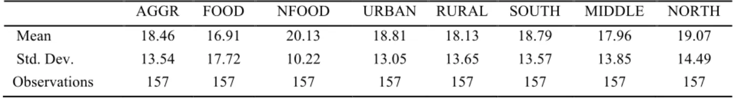
2.7.1 Descriptive statistics

The descriptive statistics in Table 2.1 show that the inflation series are not different in terms of the average and volatility. On average, inflation is highest in the non-food sector over the period with the food sector recording the lowest average inflation among all the subcomponents considered. The food inflation series happens to be the most volatile while the non-food series is the least volatile among all the subcomponents.

Table 2.1: Descriptive statistics

AGGR FOOD NFOOD URBAN RURAL SOUTH MIDDLE NORTH

Mean 18.46 16.91 20.13 18.81 18.13 18.79 17.96 19.07

Std. Dev. 13.54 17.72 10.22 13.05 13.65 13.57 13.85 14.49

Observations 157 157 157 157 157 157 157 157

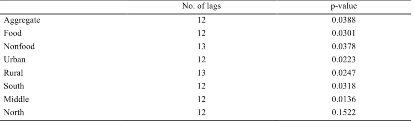
2.7.2 Time series characteristics of the series in the dataset

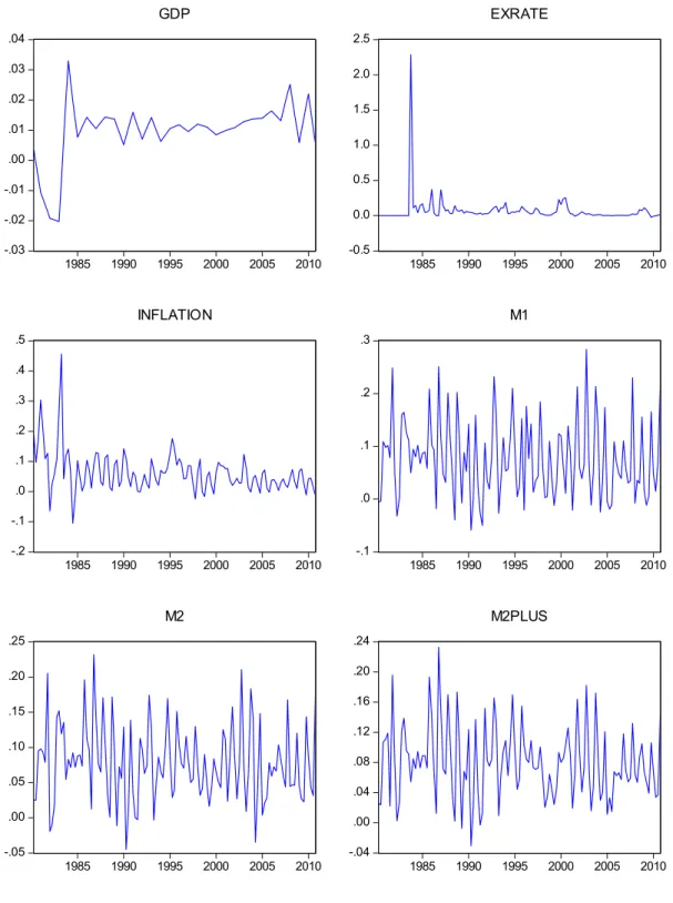
Since the ways the series are modeled depend on their time series characteristics, I investigate the series for their order of integration. The characteristics of the series are not clear from the visual examination of the graphs in Figure 2.1, so Augmented Dickey-Fuller (ADF) tests are used to determine whether the series have unit roots. Table 2.2 shows the results of the ADF tests and apart from the north series, all the series are stationary at 5 percent level of significance. This means that the series enter the models at their levels except the north series. Even though the north series is not stationary, including the first difference in the models do not produce any different result from including it at the level. I therefore treat the north series as all the other series and present the results for the levels of all the series. Similarities of the graphs also suggest that their characteristics should not be different.

(34)

Figure 2.1: Graphs of the level of the series in the dataset 0 10 20 30 40 50 60 70 2000 2002 2004 2006 2008 2010 AGGREGAT E -20 0 20 40 60 80 2000 2002 2004 2006 2008 2010 FOOD 0 10 20 30 40 50 60 2000 2002 2004 2006 2008 2010 NONFOOD -20 0 20 40 60 80 2000 2002 2004 2006 2008 2010 URBAN -20 0 20 40 60 80 2000 2002 2004 2006 2008 2010 RURAL -20 0 20 40 60 80 2000 2002 2004 2006 2008 2010 SOUT H -20 0 20 40 60 80 2000 2002 2004 2006 2008 2010 MIDDLE 0 20 40 60 80 2000 2002 2004 2006 2008 2010 NORT H

(35)

Table 2.2: Unit root tests of the variables in the data (ADF p-values)

No. of lags p-value

Aggregate 12 0.0388 Food 12 0.0301 Nonfood 13 0.0378 Urban 12 0.0223 Rural 13 0.0247 South 12 0.0318 Middle 12 0.0136 North 12 0.1522 2.7.3 Weights(

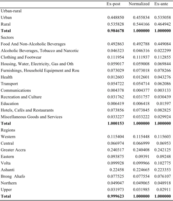
The published weights from Ghana Statistical Service suggests that the weights are constant over the sample period but analysis of the data shows that aggregating the components with the published weights do not produce the same aggregate series as published. I, therefore, compute average ex-post weight for the sample period. The ex-post weights are regression coefficient from the regression of the aggregate series on respective components corrected for serial correlation. These weights are normalized to sum to 1 and the ex-ante weights are the published weights. Table 2.3 shows the ex-post weights, normalized ex-post weights and the ex-ante weights. A major observation is the reversal of the weights for the rural-urban series, which weights the urban series more that the rural series ex-ante. The normalized ex-post weights are used in calculating the time-varying weights for aggregating the forecasts. The use of these weights as opposed to the ex-ante weights does not change the results significantly enough to change the conclusions.

(36)

Table 2.3: Weights for aggregating forecasts

Ex-post Normalized Ex-ante Urban-rural

Urban 0.448850 0.455834 0.535058

Rural 0.535828 0.544166 0.464942

Total 0.984678 1.000000 1.000000

Sectors

Food And Non-Alcoholic Beverages 0.492863 0.492788 0.449084

Alcoholic Beverages, Tobacco and Narcotic 0.046323 0.046316 0.022299

Clothing and Footwear 0.111954 0.111937 0.112855

Housing, Water, Electricity, Gas and Oth 0.059017 0.059008 0.069844 Furnishings, Household Equipment and Rou 0.073029 0.073018 0.078266

Health 0.012603 0.012601 0.043276

Transport 0.054722 0.054714 0.062086

Communications 0.004378 0.004377 0.003133

Recreation and Culture 0.031762 0.031757 0.030439

Education 0.006419 0.006418 0.01597

Hotels, Cafés and Restaurants 0.073856 0.073845 0.082825

Miscellaneous Goods and Services 0.033227 0.033222 0.029924

Total 1.000153 1.000000 1.000000 Regions Western 0.115404 0.115448 0.115603 Central 0.066974 0.066999 0.06953 Greater Accra 0.240317 0.240408 0.242125 Eastern 0.093875 0.09391 0.09248 Volta 0.099928 0.099966 0.102775 Ashanti 0.22458 0.224665 0.223353 Brong Ahafo 0.077525 0.077554 0.076107 Northern 0.049047 0.049065 0.048918 Upper 0.031973 0.031985 0.02911 Total 0.999623 1.000000 1.000000

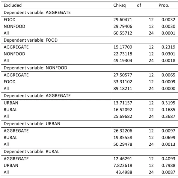
2.7.4 Granger causality tests

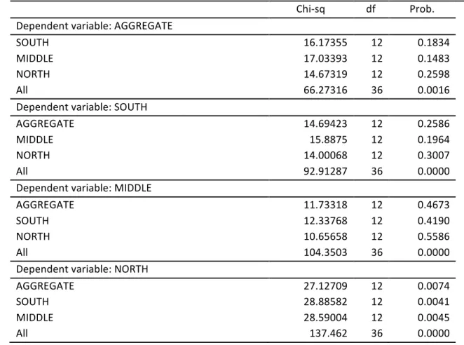
Table 2.4 is the result of Eviews’ pairwise Granger causality tests that tests whether an endogenous variable can be treated as exogenous in a particular equation. For each equation in the VAR, Table 2.4 shows chi-square statistics for the joint significance of each of the other lagged endogenous variables in that equation in column 2, degrees of freedom (df) in column 3 and p-values in column 4. The statistics in the last row (All) are for the joint significance of all other

(37)

lagged endogenous variables in the equation. The results from Table 2.4 show that food and nonfood series Granger-cause the aggregate series individually and jointly and there is a feedback from the aggregate series to nonfood but not to food series. The urban and rural series do not Granger-cause the aggregate series either individually or jointly. The aggregate series, however, Granger-cause the urban series. For the regional series, there is a strong joint Granger causality from the disaggregates to the aggregate series but none from the individual series. Feedback runs from the aggregate only to the north series. These results indicate that the food and nonfood series individually and jointly provide much information in forecasting the aggregate series but the urban and rural series do not provide much information in forecasting the aggregate series as the other disaggregates, either individually or jointly. The joint information contained of the regional series helps forecast the aggregate series but the individual series do not provide enough information to forecast the aggregate series.

(38)

Table 2.4: VAR Granger Causality/Block Exogeneity Wald Test between the aggregate and the disaggregate series

Excluded! ChiOsq! df! Prob.!

Dependent!variable:!AGGREGATE! ! ! ! FOOD! 29.60471! 12! 0.0032! NONFOOD! 29.79406! 12! 0.0030! All! 60.55712! 24! 0.0001! Dependent!variable:!FOOD! ! ! ! AGGREGATE! 15.17709! 12! 0.2319! NONFOOD! 22.73118! 12! 0.0301! All! 49.19304! 24! 0.0018! Dependent!variable:!NONFOOD! ! ! ! AGGREGATE! 27.50577! 12! 0.0065! FOOD! 33.31102! 12! 0.0009! All! 89.18211! 24! 0.0000! Dependent!variable:!AGGREGATE! ! ! ! URBAN! 13.71157! 12! 0.3195! RURAL! 16.52092! 12! 0.1685! All! 25.69682! 24! 0.3687! Dependent!variable:!URBAN! ! ! ! AGGREGATE! 26.32206! 12! 0.0097! RURAL! 19.85558! 12! 0.0699! All! 50.29478! 24! 0.0013! Dependent!variable:!RURAL! ! ! ! AGGREGATE! 12.46291! 12! 0.4093! URBAN! 7.822618! 12! 0.7988! All! 43.4988! 24! 0.0087!

(39)

Table 2.4 (Continued): VAR Granger Causality/Block Exogeneity Wald Test between the aggregate and the disaggregate series ! ChiOsq! df! Prob.! ! Dependent!variable:!AGGREGATE! ! ! ! SOUTH! 16.17355! 12! 0.1834! MIDDLE! 17.03393! 12! 0.1483! NORTH! 14.67319! 12! 0.2598! All! 66.27316! 36! 0.0016! Dependent!variable:!SOUTH! ! ! ! AGGREGATE! 14.69423! 12! 0.2586! MIDDLE! 15.8875! 12! 0.1964! NORTH! 14.00068! 12! 0.3007! All! 92.91287! 36! 0.0000! Dependent!variable:!MIDDLE! ! ! ! AGGREGATE! 11.73318! 12! 0.4673! SOUTH! 12.33768! 12! 0.4190! NORTH! 10.65658! 12! 0.5586! All! 104.3503! 36! 0.0000! Dependent!variable:!NORTH! ! ! ! AGGREGATE! 27.12709! 12! 0.0074! SOUTH! 28.88582! 12! 0.0041! MIDDLE! 28.59004! 12! 0.0045! All! 137.462! 36! 0.0000!

2.7.5 Results of the various models and model comparison

Three main models are estimated in various forms; an autoregressive (AR) model of the aggregate series and the subcomponents, a moving average (MA) of the aggregate series and the subcomponents and a vector autoregressive (VAR) model of the aggregate and the different subcomponents or all the subcomponents. The VARs are labeled by the variables that enter it, for example VAR_aggr_food means a VAR with the aggregate series and the food series as shown in Table 2.5.

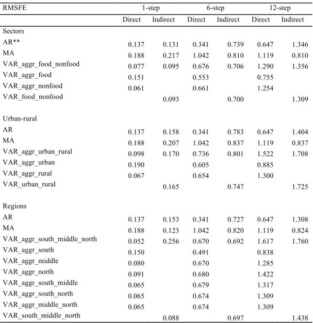
The results from the comparison of the Root Mean Squared Forecast Errors (RMSFE) from Table 2.5 show that, for all the categories considered, the benchmark autoregressive (AR) model

(40)

of the aggregate inflation series outperforms aggregate forecasts that are obtained from aggregating forecasts from the subcomponents except for the 1-step-ahead forecasts for the product sectors where aggregating the forecasts from the subcomponents perform marginally better. For the moving average (MA) models, the direct forecasts are better in all the steps except for the regions where aggregating the forecasts performs better for the 1-step-ahead.

Including additional information from the subcomponents generally performs better for all the models at 1-step-ahead forecasts. The forecasts are, however, less accurate when only food, urban or south series is included in the aggregate model individually, even for the 1-step-ahead forecasts. These results imply that the subcomponents help in producing better short-term forecasts of aggregate inflation if the right subcomponents or their combinations are used in the aggregate model. For the product sector, including the nonfood series improves the forecasts most, while including the rural series improves the forecasts most in the case of the urban-rural classification. In the case of the regional classification, including all the subcomponents improves the forecasts most.

(41)

Table 2.5: Root Mean Square Forecast Error (RMSE) for year-on-year inflation*

RMSFE 1-step 6-step 12-step

Direct Indirect Direct Indirect Direct Indirect Sectors AR** _0.137 _0.131 _0.341 _0.739 _0.647 _1.346 MA _0.188 _0.217 _1.042 _0.810 _1.119 _0.810 VAR_aggr_food_nonfood _0.077 _0.095 _0.676 _0.706 _1.290 _1.356 VAR_aggr_food _0.151 _0.553 _0.755 VAR_aggr_nonfood _0.061 _0.661 _1.254 VAR_food_nonfood _0.093 _0.700 _1.309 Urban-rural AR _0.137 _0.158 _0.341 _0.783 _0.647 _1.404 MA _0.188 _0.207 _1.042 _0.837 _1.119 _0.837 VAR_aggr_urban_rural _0.098 _0.170 _0.736 _0.801 _1.522 _1.708 VAR_aggr_urban _0.190 _0.605 _0.885 VAR_aggr_rural _0.067 _0.654 _1.300 VAR_urban_rural _0.165 _0.747 _1.725 Regions AR _0.137 _0.153 _0.341 _0.727 _0.647 _1.308 MA _0.188 _0.123 _1.042 _0.820 _1.119 _0.824 VAR_aggr_south_middle_north _0.052 _0.256 _0.670 _0.692 _1.617 _1.760 VAR_aggr_south _0.150 _0.491 _0.838 VAR_aggr_middle _0.080 _0.670 _1.285 VAR_aggr_north _0.091 _0.680 _1.422 VAR_aggr_south_middle _0.065 _0.679 _1.317 VAR_aggr_south_north _0.065 _0.674 _1.309 VAR_aggr_middle_north _0.065 _0.674 _1.309 VAR_south_middle_north _0.088 _0.697 _1.438

* Direct forecasts are the forecasts of the aggregate series from a particular model, and the indirect forecasts are the aggregate forecasts that are obtained from aggregating forecasts from the disaggregates

**The lag length for the AR varies between 1 and 3 that of the MA varies between 1 and 2 2.8 Conclusions

This study investigates whether forecasting aggregate inflations series by modeling the subcomponents performs better than forecasting the aggregate series directly, and whether

(42)

including the disaggregate components in the aggregate model improves the forecasts of the aggregate series. The benchmark model with which all the other models are compared is the univariate autoregressive (AR) of the aggregate series. The aggregate series is also modeled using moving average (MA) models. The subcomponents are modeled either independently as autoregressions (AR), moving average (MA) or jointly as vector autoregressions (VARs) with or without the aggregate series.

From the results direct forecasts of aggregate inflation outperform aggregate forecasts that are derived from aggregating forecasts from the subcomponents for all the steps of the forecasts. Including information from the subcomponents improves on the direct forecasts of the aggregate series for 1-step-ahead forecasts. This, however, depends on the subcomponents or their combinations that are used with the aggregate series. A careful selection of the subcomponents into the models is, therefore, needed to achieve more accurate forecasts. The results for 6-step-ahead and 12-step-6-step-ahead forecasts show that direct univariate forecasts are superior to the forecasts from all the models. This result should therefore be taken carefully because a longer sample is needed to evaluate more independent forecasts errors for these steps.

The results are similar to that of Hendry and Hubrisch(2010) who find that combining disaggregate information outperforms combining disaggregate forecasts. The results, however, contradict Aron and Mueller(2008) and others who find that aggregating forecasts from disaggregates is superior to direct forecasting of the aggregate series.

(43)

References

Aron, J. and N. J. Mueller(2008). "Multi-Sector Inflation Forecasting - Quarterly Models for South Africa." CSAE, WPS/2008-27.

Benalal, N.; J. L. Diaz del Hoyo; B. Landau; M. Roma and F. Skudelny(2004). "To Aggregate or Not to Aggregate? Euro Area Inflation Forecasting, ." European Central Bank Working Paper, 374.

Clemen, R. T.(1989). "Combining Forecasts: A Review and Annotated Bibliography." International Journal of Forecasting, 5, pp. 558 - 583.

de Dois Tena, J. ; A. Espasa and G. Pino(2010). "Forecasting Spanish Inflation Using Maximum Disaggregation Level by Sectors and Geographical Regions." International Regional Science Review, 33 (2), 181-204.

Fritzer, F.; G. Moser and J Scharler(2002). "Forecasting Austrian Hicp and Its Components Using Var and Arima Models." Oesterreichische Nationalbank working paper http://www.oenb.co.at/workpaper/pubwork.htm, 73.

Granger, C. W. J.(1969). "Investigating Causal Relations by Econometric Models and Cross-Spectral Methods " Econometrica, 37, pp. 424 - 438.

Grunfeld, Y and Z. Griliches(1960). "Is Aggregation Necessarily Bad?" Review of Economics and Statistics, XLII(1), 1-13.

Hendry , D. F. and K. Hubrisch(2005). " Forecasting Aggregates with Disaggregates." http://www.nuff.ox.ac.uk/users/hendry/HendryHubrich05.pdf, Manuscript.

Hendry , D. F. and K. Hubrisch(2010). "Combining Disaggregate Forecasts or Combining Disaggregate Information to Forecast an Aggregate " European Central Bank Working Paper Peries, No. 1155, pp. 1 - 32

Hendry , D.F and K. Hubrsch(2005). "Forecasting Aggregates with Disaggregates." Manuscript.

Hubrisch, K. (2003). " Forecasting Euro Area Inflation: Does Aggregating Forecasts by Hicp Components Improve Forecast Accuracy? ." European Central Bank Working Paper 247.

Judge, G. G.; W. E. Griffiths; R. C. Hill; H. Lutkepohl and T. C. Lee(1988). Introduction to the Theory and Practice of Econometrics. John Wiley & Sons Inc.

Kohn, J(1982). "When Is Aggregation of a Time Series Efficiently Forecast by Its Past?" Journal of Econometrics, 18(2002), 337-349.

Lutkepohl, H. (1984). "Forecasting Contemporaneously Aggregated Vector Arma Processes." Journal of Business & Economic Statistics, 2(3), 201-214.

(44)

Pesaran, M.H.; R.G. Pierse and M.S. Kumar(1989). "Econometric Analysis of Aggregation in the Context of Linear Prediction Models." Econometrica, 57(4), 861-888.

Theil, H(1954). "Linear Aggregationof Economicrelations." Amsterdam: North-Holland.

van Garderen, K.J.; K. Lee and M.H. Pesaran(2000). "Cross-Sectional Aggregation of Non-Linear Models." Journal of Econometrics, 95 (2000), 285-331.

Zellner, A. and J Tobias(2000). "A Note on Aggregation, Disaggregation and Forecasting Performance." Journal of Forecasting, 19, 457-469.

(45)

3 CHAPTER 3: SEPARATING MONETARY AND STRUCTURAL CAUSES OF INFLATION.

3.1 Introduction and theoretical framework

There are two schools of thought on what explains inflation; monetary growth or structural factors. The monetarist school argues that money is all that matters in explaining inflation. This forms the basis of the monetarist statement that “inflation is always and everywhere a monetary phenomenon”. The structuralist school, on the other hand, argues that structural and institutional factors play a more prominent role in inflation dynamics. The structuralists’ argue that inelastic food supply, infrastructural inadequacies that pose problems for distribution of output, lack of financial resources and low export receipts leading to foreign exchange shortages in developing countries put pressure on domestic prices (London(1989)). “The nominal exchange rate pass-through to domestic price inflation depends on how the changes in the exchange rates are passed through to import prices and therefore to domestic consumer prices” (Mishkin(2008)). It is also argued that the lack of financial resources coupled with a limited tax base cause these less developed countries to resort to deficit financing through the central banks, that lead to inflationary pressures.

This study uses a structural vector autoregression to model inflation so as to identify the relative importance of monetary and structural factors in explaining inflation in developing countries by using data from Ghana. Specifically, this paper explores three things; first, the paper identifies the relative importance of output supply shocks, monetary growth shocks and exchange rate depreciation shocks in inflation dynamics by analyzing the variance decomposition of the forecast error variance of inflation. Secondly, the paper analyzes how shocks to real output growth, monetary growth and exchange depreciation transmit through to price developments and

(46)

how fast these shocks dissipate. Lastly, the paper identifies what other channels of monetary policy transmission mechanisms exist in Ghana’s monetary policy framework over the years. These help identify which of the variables has more information in better management of inflation in Ghana.

In 2002, Ghana adopted inflation targeting as its monetary policy framework, which requires appropriate target setting for inflation. The adoption of the inflation-targeting framework has certain prerequisites and technical issues as outlined in Blejer and Leone(2000). Among these prerequisites and technical issues are a clear understanding of the monetary policy transmission mechanism and reliable forecasts of inflation. This shows that setting appropriate inflation targets require not only accurate forecast but also knowledge of the channels through which policy variables affect inflation. The knowledge of the impact of these policy variables on inflation also helps in the efficient policy formulation to achieve the target. Also, “a successful implementation of any monetary policy regime requires an accurate and informed assessment of how fast the effects of policy changes propagate to other parts of the economy and how large these effects are. This requires a thorough understanding of the mechanism through which monetary policy actions and other forms of shocks affect economic activity” (Abradu-Otoo et al.(2003)). So knowing the forecast values from the univariate time series models is necessary but not sufficient for the inflation targeting monetary policy framework adopted by the Bank of Ghana.

3.2 Literature on inflation in Africa

The monetarists-structuralists debate makes it hard to determine what actually causes inflation, especially in Africa where structural factors are more highlighted. Some studies find that neither

(47)

monetary nor structural factors alone explain inflation completely especially in Africa. Among the most relevant studies on monetary growth, exchange rate and inflation nexus in Africa are Chhibber et al.(1989), London(1989), Tegene(1989), Canetti and Greene(1991) and Imimole and Enoma(2011). Chhibberet al.(1989) observe that inflationary process goes beyond simple monetary explanation and identify three transmission mechanisms for the inflationary dynamics in Zimbabwe. First, cost-push factors such as nominal wage changes, pass-through effect of import prices and government price controls impact domestic prices directly. Secondly, excess money supply interactions with modes of deficit financing translate into pressure on prices and finally, unfavorable supply conditions pressure prices. London(1989) uses both cross-section data over several African countries and time series data for individual countries and finds that monetarists view on inflation holds in the cross-section equations but not in the individual time series models for all the countries. London(1989) sug