Statistical Inference Based on Upper Record Values

(1)

W&M ScholarWorks

Undergraduate Honors Theses Theses, Dissertations, & Master Projects

6-2013

Statistical Inference Based on Upper Record Values

Daniel J. Luckett

College of William and Mary

Follow this and additional works at: https://scholarworks.wm.edu/honorstheses

Recommended Citation Recommended Citation

Luckett, Daniel J., "Statistical Inference Based on Upper Record Values" (2013). Undergraduate Honors Theses. Paper 577.

https://scholarworks.wm.edu/honorstheses/577

This Honors Thesis is brought to you for free and open access by the Theses, Dissertations, & Master Projects at W&M ScholarWorks. It has been accepted for inclusion in Undergraduate Honors Theses by an authorized administrator of W&M ScholarWorks. For more information, please contact [email protected].

(2)

Statistical Inference Based on Upper Record Values

A thesis submitted for partial fulfillment of the requirements for the degree of Bachelor of Science in Mathematics from

The College of William and Mary

by Daniel J. Luckett Accepted for

f/

o

r

tO

r

s

~~

Y;I-Tanujit Dey

:

9 &~.

Ross J. laci

~-'

---

-~

7

_{Lawrence M. Leemis}

~

Williamsburg, VA 24 April, 2013

(3)

Acknowledgments

I would like to thank my thesis advisor, Dr. Tanujit Dey, as well as the thesis committee members, Dr. Lawrence M. Leemis, Dr. Ross J. Iaci, and Dr. M. Drew LaMar. I would also like to thank Dr. Sanku Dey for his valuable contributions to this research. Finally, I would like to thank the many faculty members at the William & Mary Mathematics Department, too numerous to name.

(6)

Abstract

The goal of this thesis is to examine methods of statistical inference based on upper record values. This includes estimation of parameters based on samples of record values and prediction of future record values. We first define and discuss record times and record values and their distributions. Then we propose an efficient algorithm to generate random samples of record values. The algorithm, based on the conditional survivor function, has a time complexity that is linear with respect to the sample size. It is quite efficient and can be useful in simulation. Next, we discuss inference prob-lems related to two distributions, the generalized inverted exponential distribution and the generalized Rayleigh distribution. A number of techniques are considered, including both frequentist and Bayesian techniques. The following are considered for each of these two distributions. We first consider maximum likelihood and Bayesian estimation of the unknown parameters based on upper record values. We also con-sider empirical Bayes estimation. Then, we derive approximate confidence intervals based on a normal approximation, bootstrap confidence intervals, and two-sided Bayes probability intervals based on record values. We derive both maximum likelihood and Bayesian methods for predicting future record values. Numerical results include both simulation and data analysis. We conduct a simulation study for each distribution. Simulation is used to compare the performance of maximum likelihood estimators, Bayesian estimators, and empirical Bayes estimators. We consider the average bias and mean squared error for these estimators. We also consider the average length and coverage probability for approximate confidence intervals. As many of the results in this paper cannot be found in closed form, we use numerical methods to find the maximum likelihood estimates and we implement the Metropolis–Hastings algorithm to compute the Bayes estimates. We use each distribution to model one real data set by estimating the parameters, computing approximate confidence intervals and two-sided Bayes probability intervals, and evaluating the fit. Finally, we illustrate Bayesian prediction methods on a simulated sample for each distribution.

(7)

Chapter 1 Introduction

1.1 Overview and Motivation

Record values and record times have been of interest to humans throughout his-tory. Meteorologists frequently deal with upper and lower record temperatures and precipitation levels. A seismologist may be interested in earthquakes of record magni-tude. Record values appear often in sporting events. For example, an analyst may be concerned with record performances in the Olympic one hundred meter dash. There is something about record breaking performances that makes them fascinating to humans. Thus, it is natural to try to quantify the study of records in a statistical sense.

The study of statistical records ﬁrst emerged in a landmark paper by Chandler (1952). Numerous papers on records were published throughout the 1950s. A number of statisticians have worked on interesting problems pertaining to the study of records. Wilks (1959) posed the question of how many additional observations are needed to observe a value exceeding the maximum of nobservations. R´enyi (1962) showed that record times are independent. The notion ofkth record times was introduced by Dz-iubdziela and Kopocinsky (1976). Weak records were introduced by Vervaat (1973). Arnold et al. (1998) give a likelihood function for estimating unknown parameters based on record samples. Basak and Balakrishnan (2003) give a predictive likelihood function for future record values.

A number of statisticians have studied inference based on record samples for cer-tain distributions. Doostparast (2009) and Jaheen (2004) studied the exponential distribution. Doostparast and Ahmadi (2006) studied the geometric distribution. For an overview of the theory of records see Nevzorov (2001). Ahsanullah (1995) contains an overview of records along with applications to a wide variety of distributions.

The goal of this paper is to study statistical inference based on upper record val-ues for the generalized inverted exponential distribution (GIED) and the generalized

(8)

Rayleigh (GR) distribution. Frequentist and Bayesian methods are used to estimate unknown parameters and predict future record values. After introducing theoretical results pertaining to inference based on records, we assess the performance of diﬀer-ent estimators and predictors using simulation. Multiple real data sets are used for illustrative purposes. As simulation is such an important part of this research, we address the problem of generating samples of record values by proposing an eﬃcient algorithm to generate record samples.

There are many situations where a data set may consist of only record values. As an example, consider a sporting event where only record-breaking performances are recorded. The analyst needs to ﬁt a model to the data when the record values are known but the whole sample is not. Such situations require an ability to accurately estimate parameters of a distribution based only on a record sample. There are many situations where the prediction of future records is essential. A meteorologist may want to know how much ﬂooding will occur the next time the current rainfall record is broken. The statistician must estimate the next record value of rainfall from a data set consisting of past record values. The goal of this paper is to evaluate methods for inference and prediction problems like these.

This thesis is organized as follows. The rest of Chapter 1 deﬁnes the mathemat-ical properties of record times and record values and their distributions. Chapter 2 proposes an algorithm to quickly and eﬃciently generate samples of record values. Chapters 3 and 4 discuss statistical inference based on upper records for the gen-eralized inverted exponential distribution and the gengen-eralized Rayleigh distribution, respectively. The results presented are compared using simulation and data analysis.

1.2 Applications of Records

The mathematical theory of records has extensive applications to real world situ-ations. We will consider two of them here as motivating examples. First, consider an example from reliability theory. Suppose we have a system ofnidentical components such that the system functions when k or more out of the n components are func-tioning. Thus, the system will fail when the (n₋k+ 1)th component fails. Note that this includes the cases of series and parallel systems when k=n and k= 1, respec-tively. There are many examples of systems that ﬁt this description. Suppose we are interested in predicting the lifetime of the system whenr components have failed, for some 1_≤r < k_≤n. The lifetime of the system corresponds to the (n₋k₋r+ 1)th future record value.

(9)

As a second example, consider a Type-II censoring scheme. Suppose there are n

items on test and the test will conclude after k failures, for some k < n. It may be of interest to predict how long the test will last. To do this, one must predict the

kth future record value. Such a situation would occur, for example, in an accelerated life test to test the lifetime of mechanical components, when the failure time for each component is recorded. Alternatively, the same situation would occur in a clinical trial when the time at which a patient is cured is recorded.

1.3 Deﬁnition of Upper and Lower Records

Suppose that X1, X2, . . . is a sequence of independent and identically distributed

(iid) random variables from a continuous distribution. We say that Xi is an upper

record value and i is an upper record time ifXi > Xj for all j < i. In other words,

an upper record value is a value that is greater than all observed values so far. The record times are the indices at which record values occur. We note that, by this deﬁnition, an observation must be strictly greater than and not equal to the previous upper record in order to be considered a record value.

To formalize this notion, let X1, X2, . . . , Xn be a random sample of sizen from a

continuous distribution. Deﬁne the ﬁrst record time, U(1) = 1 and the mth record time, for m >1 by the recursive formula

U(m) = min{j > U(m−1) :Xj > XU(m−1)}.

The mth record value, then, isXU(m).

Next we will deﬁne the notion of kth records. Let X1, X2, . . . , Xn be a random

sample of size nfrom a continuous cumulative distribution function. Deﬁne the ﬁrst

kth record time as U(1, k) = k and the mth kth record time, for m > 1 by the recursive formula

U(m, k) = min{j > U(m−1, k) :Xj > XU(j−k,k−1)}.

For details on kth records, see Nevzorov (2001).

Finally, we say that Xi is a weak record if Xi ≥ Xj for all j < i. Weak records

generalize the notion of records by including as an upper record any observation that is equal to the most recent upper record. This corresponds to the situation where a record is “tied” but not “broken.” Analogous deﬁnitions for all of these exist for lower records as well.

An important question that arises is that of how many records one should expect to observe in a sample of size n. Let Mn be the number of record observations in a

(10)

random sample of size n. It is shown in Ahsanullah (1995), that the expected value of Mn is E[Mn ] = n ∑ i=1 1 i.

Thus, in a sample of size n, one can expect to see only approximately logn record values (Doostparast (2009)).

Another interesting question is that of how long one would expect to wait before observing a new upper record. Wilks (1959) addresses this question. For a random sample of size n, letN(n) be the minimum number of additional observations needed in order to observe a value greater than Mn = max{X1, X2, . . . , Xn}. Let N(1) be

the minimum number of additional observations needed in order to observe a value less than mn = min{X1, X2, . . . , Xn}. Deﬁne N(1, n) as the minimum number of

additional observations needed to observe a value that falls outside of the interval [mn, Mn]. It is shown in Nevzorov (2001) that while E[N(1, n)] = n, E[N(1)] =

E[N(n)] = _∞. Thus, the expected time to observe a new record value is inﬁnite. These two results show how diﬃcult it can be to generate simulated samples of record values.

1.4 Distributions of Record Times and Record

Val-ues

We will now derive the distributions of record times and record values. We will concern ourselves only with upper records. Results for lower records can be derived analogously.

1.4.1 Record Times

Let U(1) = 1 be the ﬁrst record time. Nevzorov (2001) shows that the survivor function of the second record time is

S2(j) =P

(

U(2)> j)= 1

j j= 1,2, . . . .

Thus, the probability mass function of U(2) is

f2(j) =P

(

U(2)> j₋1)₋P(U(2)> j)= 1

j(j−1) j = 2,3, . . . . We know from R´enyi (1962) that record times are independent. Thus, the joint probability mass function of the ﬁrst n record times is

f(j2, j3, . . . , jn) =P ( U(1) = 1, U(2) =j2, . . . , U(n) =jn ) = 1 (j2−1)(j3−1)· · ·(jn−1)(jn) ,

(11)

for 1 =j1 < j2< . . . < jn. The marginal probability mass function of themth record time is fm(j) = ∑ 1<k2<...<km−1<j 1 (k2−1)(k3−1)· · ·(j−1)(j) .

It can be shown that record times U(1), U(2), . . .form a Markov chain.

Along with the record times U(i), we can deﬁne the inter-record times ∆(1) = 1 and ∆(i) =U(i)−U(i−1) for i > 1. Inter-record times correspond roughly to the number of non-record observations between record values. Nevzorov (2001) shows that the inter-record times are conditionally independent given the record values, and the ith inter-record time has probability mass function

fi(m) =P ( ∆(i) =m_|XU(1), XU(2), . . . ) =(1₋F(XU(i−1)) )( F(XU(i−1)) )m−1 ,

form= 1,2, . . ., and i= 2,3, . . . .Thus, theith inter-record time follows a geometric distribution.

1.4.2 Record Values

Let X1, X2, . . .be a sequence of iid random variables with continuous cumulative

distribution function F and probabilty density function f. The survivor function of the mth record value, XU(m), given the past record values XU(1), XU(2), . . . , XU(m−1),

is Fm(x) =P ( XU(m)> x|XU(2) =x2, XU(3)=x3, . . . , XU(m−1)=xm−1 ) = 1−F(x) 1−F(xm−1) .

The conditional density function is

fm(x|x1, x2, . . . , xm−1) =

f(x) 1−F(xm−1)

.

It follows that record values form a Markov chain as well. The joint probability density function of the record values XU(1), XU(2), . . . , XU(n) is

fn(x1, x2, . . . , xn) =

f(x1)f(x2)· · ·f(xn)

(1₋F(x1))(1−F(x2))· · ·(1−F(xn−1))

.

This joint density function is important for maximum likelihood estimation based on record values.

Nevzorov (2001) notes one more important result dealing with extending the probability integral transformation to record values. Let X1, X2, . . . , Xn be the ﬁrst

n upper record values from a continuous cumulative distribution function, F. Let

U1, U2, . . . , Un be the ﬁrstn upper record values from a uniform distribution on the

interval [0,1]. Then, the random vector (F(X1), F(X2), . . . , F(Xn)) has the same

(12)

The mathematical theory of records is a growing area of study with great potential for research. The results we have presented comprise only a small number of the developments that have been made.

(13)

Chapter 2 An Eﬃcient Algorithm for

Generating Record Values

2.1 Introduction

The study of record values is popular in many areas because of its wide applicabil-ity in the modeling and analysis of lifetime data. Motivated by the study of extreme weather conditions, Chandler (1952) introduced the study of record values and doc-umented many of the basic properties of records. There is a volume of statistical literature on the subject of record statistics, and the underlying theory for the likeli-hood of a record-breaking event taking place in a stable system is remarkably simple (see Benestad (2003)). Properties of record values have been extensively studied in the literature by Ahsanullah (1988, 1995), Arnold and Balakrishnan (1989), Arnold et al. (1992, 1998), Nevzorov (2001), Kamps (1995) and Jaheen (2004).

Simulation studies are an integral part of statistical research. Simulation is used advantageously in a number of situations. This includes providing the empirical es-timation of sampling distributions, studying the misspecification of assumptions in statistical procedures, determining the power in hypothesis tests, and many others. However, in order to design simulation studies relating to record values, one must be able to efficiently generate record samples from a wide variety of distributions. Doostparast (2009) claims that from a sequence of n independent and identically distributed random variables, only about logn variates will be record values. Al-gorithms that generate records by generating n random variates and accepting only those which are record values are very inefficient. To the best of our knowledge, there is no algorithm at hand that can efficiently generate record values from several distributions. Given this condition, generating moderately large samples of record values or a large number of samples of record values will take a significant amount of time. A vast amount of research has been conducted where simulation studies have

(14)

been carried out only based on small samples. Simulation studies come with their own set of limitations. In the framework of multilevel studies an important problem is generating an adequate sample size that provides unbiased and accurate estimates. In this chapter we present an eﬃcient algorithm for generating records that is based on the conditional survivor function and will work for any distribution with a closed form inverse survivor function. We proceed as follows. Section 2.2 discusses the algorithm for upper record values and section 2.3 discusses the analogous case for lower record values. Section 2.4 contains an example for implementing our algorithm. We conclude with ﬁnal remarks in section 2.5.

2.2 Algorithm for Upper Records

Let X be a random variable with population probability density function f(x) on positive support and cumulative distribution function F(x). We wish to generate a random sample of n upper records from the distribution of X. That is, we need a sample xU(1), xU(2), . . . , xU(n) where xU(i) is drawn from the distribution of X and

xU(i) < xU(j) for all i < j. This is challenging because it may take many repeated

sample points before nupper records are generated, even for relatively small n. We set the condition that each record value xU(i) is greater than xU(i−1). Thus,

the ﬁrst sample point generated will be the ﬁrst upper record, xU(1). The second

upper record is obtained by sampling from the conditional distributionFX|X>xU(1)(x).

Iterating this process will yield a random sample of upper records, where each record is drawn from the desired distribution and each record is greater than all those before it. Assuming that random variates can be generated from the distribution of X

and that the conditional distribution of X is easily obtained, each iteration can be performed in constant time. Thus, the entire algorithm has a time complexity that is linear with respect to the desired sample sizen. Next, we show how this algorithm can be easily implemented for a variety of distributions.

Assuming that the distribution of X has survivor function S(x) and inverse sur-vivor function S−1₍_x_{) that can be obtained in closed form, it is well known that a}

simple variate generation algorithm for X is generateU ∼U(0,1)

return X=S−1₍_U₎

(15)

known that the conditional survivor function of X given that X > t is

SX|X>t(x) =

S(x)

S(t) x > t. The inverse of the conditional survivor function is found as

S_X−1_|_X>t(x) =S(t)S−1(x) x > t.

So, an eﬃcient algorithm for generating a random sample of upper records can be obtained as in Algorithm 1.

Algorithm 1 To generate upper records

1: generate U ∼U(0,1) 2: calculate X1=S−1(U) 3: for i= 2 tondo 4: generateU ∼U(0,1) 5: calculate Xi=S(Xi−1)S−1(U) 6: end for 7: return X1, X2, . . . , Xn

8: the sample X1, X2, . . . , Xn will represent n upper record values

(xU(1), xU(2), . . . , xU(n)) =0

2.3 Algorithm for Lower Records

Here we propose an analogous algorithm for generating samples of lower records. Let X be a random variable with probability density function f(x) on positive sup-port and cumulative distribution function F(x). We wish to generate a random sample of lower records from the distribution of X. That is, we need a sample

xL(1), xL(2), . . . , xL(n)wherexL(i)is drawn from the distribution ofX andxL(i)> xL(j)

for all i < j.

An analogous algorithm can be deﬁned for generating samples of lower records. Assume that the distribution of X has survivor function S(x), inverse survivor func-tionS−1₍_x_{), and cumulative distribution function}_F₍_x_{) that can be obtained in closed}

form. The conditional survivor function given that X is less than tis given by

SX|X<t(x) =

S(x)

F(t) x < t. The inverse of the conditional survivor function is found as

S_X−1_|_X>t(x) =F(t)S−1(x) x < t.

So, an algorithm for generating a random sample of lower records can be obtained as in Algorithm 2.

(16)

Algorithm 2 To generate lower records 1: generate U _∼U(0,1) 2: calculate X1=S−1(U) 3: for i= 2 tondo 4: generateU _∼U(0,1) 5: calculate Xi=F(Xi−1)S−1(U) 6: end for 7: return X1, X2, . . . , Xn

8: the sample X1, X2, . . . , Xn will represent n lower record values

(xL(1), xL(2), . . . , xL(n)) =0

2.4 Illustration and Analysis

As an example, we can easily implement the above algorithms for the one pa-rameter exponential distribution as follows. Let X be an exponentially distributed random variable with parameterλ with survivor function

S(x) =e−λx x_≥0. Then, SX|X>t(x) = e−λx e−λt =e −λ(x−t) _x ≥t.

So the corresponding inverse survivor function is

S−1(u) =₋log(u)/λ,

whereuis a sample from theU(0,1) distribution. So, the inverse conditional survivor function is

S_X|X>t−1 (u) =S(t)S−1(u) =₋e

−λt_log(_u₎

λ .

We can now use Algorithm 1 to generate a sample of upper records from the expo-nential distribution. The algorithm is reasonably eﬃcient. We have implemented and executed our algorithm in R software to generate upper records from the exponen-tial(1) distribution. The running times (in seconds) for generating a sample of upper records of size n from an exponential(1) is shown in Table 2.1. A plot of execution times against the sample size appears in Figure 2.1.

n 1000 2000 3000 4000 5000

Time 0.0115 0.0266 0.0435 0.0641 0.0857

Table 2.1: Execution times (in seconds) for generating exponential(1) upper record samples

Table 2.1 and Figure 2.1 both provide visual evidence that the proposed algorithm achieves a linear time complexity. Running times featured in Table 2.1 and Figure 2.1 are average running times over 100 executions of the algorithm for each sample size.

(17)

0 1000 2000 3000 4000 5000 0.000 0.025 0.050 0.075 n t

Figure 2.1: Plot of execution time against sample size

The execution time grows no faster than linearly with respect to the sample size. Any algorithm that produces random data must go through a certain degree of exer-tion to generate each value. In other words, the number of steps required to produce

n values must be a linear function ofn. Thus, any algorithm that produces random data must feature an execution time that grows linearly with respect to the sample size, and one would not expect any algorithm to achieve a better time complexity than the algorithm presented here.

2.5 Conclusion

Statistical research involving record values is vital as it has countless applications in several areas. Simulation studies are an imperative part of this research. However, an eﬃcient variate generation algorithm is needed to perform any kind of simulation study. In the past, record samples have been generated by constructing many sample points and accepting only those random variates which are records. This technique is vastly wasteful and inept. In this chapter we propose a faster algorithm for generating records. It is simple and easy to implement under any circumstances. The algorithm presented here generates record samples for large sample sizes in milliseconds. Even for sample sizes as large as n = 5000, the algorithm executes in under 0.1 seconds. This algorithm should greatly improve computational eﬃciency for simulation studies related to record data.

(18)

Chapter 3 Statistical Inference for the

Generalized Inverted Exponential

Distribution Based on Upper

Record Values

3.1 Introduction

The study of record values and associated statistics are of great signiﬁcance in many real life situations such as meteorology, seismology, athletic events, economics, and life testing. The frequency of weather conditions inspired Chandler (1952) to study the distributions of lower records, record times, and inter-record times for indepen-dent and iindepen-dentically distributed (iid) sequences of random variables. Since then, numerous papers on record values and their distributional properties have appeared in the statistical literature. Among them are Ahsanullah (1988, 1995), Arnold and Balakrishnan (1989), Arnold et al. (1992, 1998), and Kamps (1995).

LetXU(1), XU(2), . . . , XU(n)be the ﬁrstnupper record values from the two-parameter

generalized inverted exponential distribution (GIED) with probability density func-tion

f(x;α, λ) = αλ

x2e

−λ/x₍₁

−e−λ/x)α−1 x≥0, α, λ >0 (3.1) and cumulative distribution function

F(x;α, λ) = 1₋(1₋e−λ/x)α x_≥0. (3.2) The hazard function, then, is

h(x;α, λ) = αλ

x2₍_eλ/x₋₁₎ x≥0. (3.3)

Here α, λ > 0 are the shape and scale parameters, respectively. The generalized in-verted exponential distribution with shape parameterαand scale parameterλwill be

(19)

denoted by GIED(α, λ). The generalized inverted exponential distribution (GIED) was introduced in the literature by Abouammoh and Alshingiti (2009) as a general-ization of the inverted exponential distribution. Abouammoh and Alshingiti (2009) carried out extensive studies on the properties of the GIED. Due to its practicality, the GIED can be used for many applications, including accelerated life testing, horse racing, supermarket queues, sea currents, wind speeds, and others (see Nadarajah and Kotz (2000)). The hazard function of the GIED can never be constant. The GIED has a unimodal and right skewed density function. Abouammoh and Alshingiti (2009) observed that in many situations, the GIED provides a better ﬁt than the gamma, Weibull, generalized exponential, and inverted exponential distributions. Plotted be-low on the left are probability density functions for the GIED with α = 1, λ = 1 plotted as the solid line, α= 2, λ= 1 plotted as the dashed line, and α=.25, λ= 1 plotted as the dotted line. Plotted on the right are various hazard functions for the GIED using the same parameter settings.

0 1 2 3 4 0.0 0.2 0.4 0.6 0.8 1.0 f(x) x

Figure 3.1: GIED density functions

0 1 2 3 4 0.0 0.5 1.0 1.5 h(x) x

Figure 3.2: GIED hazard functions Recently, Krishna and Kumar (2012) studied the reliability estimation of this distribution under progressive type-II censoring.

The rest of this chapter is organized as follows. In Section 3.2, we derive the maximum likelihood estimators for the two unknown parameters of the GIED. In Section 3.3 we derive the Bayes estimators based on the general entropy loss function. Section 3.4 presents the predictive distribution of the future record values based on a given set of the ﬁrstnupper records. Numerical comparison results and data analysis are presented in Section 3.5. We conclude in Section 3.6.

(20)

3.2 Non-Bayesian Estimation

In this section we discuss the process of obtaining the maximum likelihood estimators of the parametersαandλbased on upper record values. LetX1, X2, . . .be a sequence

of independent and identically distributed random variables with cumulative distri-bution functionF(x) and probability density function f(x) on positive support. Let

Yn = max{X1, X2, . . . , Xn}forn≥1. The observationXj is an upper record value of {Xi}i≥1 if it is greater than all preceding observations, that is, ifYj > Yj−1 forj >1.

Suppose we observe n upper record values X = {XU(1), XU(2), . . . , XU(n)} from

a sequence of iid random variables following a GIED(α, λ) with probability density function in (3.1). Arnold et al. (1998) give the likelihood function as

L(α, λ_|x) =f(xU(n);α, λ) n−1 ∏ i=1 f(xU(i);α, λ) 1₋F(xU(i);α, λ) 0_≤xU(1)< xU(2)< . . . < xU(n)<∞. (3.4) Substituting (3.1) and (3.2) in (3.4), we get the likelihood function

L(α, λ_|x) =αnλneαln ( 1−e−λ/xU(n))∏n i=1 1 x2 U(i) · e −λ/xU(i) 1₋e−λ/xU(i). (3.5)

The maximum likelihood estimates are the values of α and λ that maximize this likelihood function.

3.2.1 Maximum Likelihood Estimation

The log likelihood function ℓ(α, λ|x) = logL(α, λ|x), dropping terms that do not involve αandλ, is ℓ(α, λ|x) =n(ln α+ ln λ)− n ∑ i=1 λ xU(i) +αln(1−e−λ/xU(n))− n ∑ i=1 ln(1−e−λ/xU(i))_. (3.6) We assume that the parametersαandλare unknown. To obtain the normal equations for the unknown parameters, we diﬀerentiate (3.6) partially with respect to αandλ

and equate to zero. The resulting equations are

0 = ∂ℓ ∂α = n α+ ln ( 1−e−λ/xU(n)) _(3.7) and 0 = ∂ℓ ∂λ = n λ− n ∑ i=1 1 xU(i) +α e −λ/xU(n) xU(n) ( 1−e−λ/xU(n))− n ∑ i=1 e−λ/xU(i) xU(i) ( 1−e−λ/xU(i)). (3.8)

(21)

The solutions of the above equations are the maximum likelihood estimators of the GIED parameters αandλ, denoted ˆαM LE and ˆλM LE, respectively. As the equations

expressed in (3.7) and (3.8) cannot be solved analytically, one must use a numerical procedure to solve them.

3.2.2 Approximate Conﬁdence Intervals

Since the maximum likelihood estimators of the unknown parametersαandλcannot be derived in closed form, it is not easy to derive the exact distributions of the MLEs. Hence, we cannot obtain exact conﬁdence intervals for the parameters. We must use the large sample approximation. It is known that the asymptotic distribution of the MLE ˆθ is (ˆθ₋θ)_→ N2(0, I−1(θ)) (see Lawless (1982)), where I−1(θ), the inverse of

the observed information matrix of the unknown parameters θ= (α, λ), is

I−1(θ) = ( −∂2ℓ(∂αα,λ|x2 ) − ∂2_ℓ₍_α,λ|x₎ ∂α∂λ −∂2ℓ∂λ∂α(α,λ|x) − ∂2_ℓ₍_α,λ_|_x₎ ∂λ2 ) −1 (α,λ)=( ˆα,ˆλ) = ( var(ˆα) cov(ˆα,λˆ) cov(ˆλ,αˆ) var(ˆλ) ) .

The derivatives in I(θ) are given by

∂2_ℓ₍_{α, λ} |x) ∂α2 = − n α2 (3.9) ∂2_ℓ₍_{α, λ}_|_x₎ ∂α∂λ = e−λ/xU(n) xU(n) ( 1−e−λ/xU(n)) = ∂2_log_L ∂λ∂α (3.10) ∂2_ℓ₍_{α, λ}_|_x₎ ∂λ2 =− n λ2 −α e−λ/xU(n) x2 U(n) ( 1₋e−λ/xU(n))2 + n ∑ i=1 e−λ/xU(i) x2 U(i) ( 1₋e−λ/xU(i))2 . (3.11) The above approach is used to derive approximate 100(1₋τ)% conﬁdence intervals of the parameters αandλof the forms

ˆ α_±zτ /2 √ var(ˆα) and ˆ λ±zτ /2 √ var(ˆλ),

(22)

3.2.3 Bootstrap Conﬁdence Intervals

Here we present bootstrap conﬁdence intervals for the GIED. First, we will use a bootstrap method based on percentiles as presented in Efron (1982). The algorithm uses the following steps.

1. From the sample xU(1), xU(2), . . . , xU(n), compute the maximum likelihood

esti-mates ˆαand ˆλ.

2. Generate a bootstrap samplex∗

U(1), x∗U(2), . . . , xU∗(n), using ˆαand ˆλas parameters.

3. Compute the maximum likelihood estimates ˆα∗

1 and ˆλ∗1 based on the bootstrap

sample.

4. Repeat steps 2 and 3 N times, and store ˆα∗i and ˆλ∗i from step 3 for i =

1,2, . . . , N. 5. Arrange the ˆα∗

i in ascending order and obtainαU andαL, the upper and lower

limits of a 100(1₋γ)% bootstrap conﬁdence interval for α, as the γ/2 and (1₋γ/2) percentiles of the ˆα∗

i.

6. Arrange the ˆλ∗

i in ascending order and obtain λU andλL, the upper and lower

limits of a 100(1₋γ)% bootstrap conﬁdence interval for λ, as the γ/2 and (1−γ/2) percentiles of the ˆλ∗i.

A second bootstrap method is based on Hall (1988). The algorithm proceeds as follows.

3. Based on the bootstrap sample, compute the maximum likelihood estimates, ˆα∗

and ˆλ∗_{, as well as the statistics.}

T₁∗= √ n(ˆα∗₋_α_ˆ₎ √ V ar(ˆα∗₎ and T ∗ 2 = √ n(ˆλ∗₋_λˆ₎ √ V ar(ˆλ∗₎

where V ar(ˆλ∗_{) and} _{V ar}_(ˆ_α∗_{) are found from the observed Fisher information}

matrix.

(23)

5. For the values ofT∗

1 andT2∗ found in step 3, let F(x) =P(Ti∗ < x), fori= 1,2

be the cumulative distribution function ofT∗

1 andT2∗. Deﬁne ˆ αt(x) = ˆα+ √ V ar(ˆα) √ n and ˆλt(x) = ˆλ+ √ V ar(ˆλ) √ n

whereV ar(ˆλ) andV ar(ˆα) are also found from the observed Fisher information matrix.

6. Approximate 100(1−γ)% conﬁdence intervals ofαand λare given by

( ˆ αt(γ/2),αˆt(1−γ/2) ) and (ˆλt(γ/2),λˆt(1−γ/2) ) .

These bootstrap conﬁdence intervals provide an alternate to the approximate con-ﬁdence intervals derived in Section 3.2.2.

3.3 Bayesian Estimation

In this section we consider Bayesian inference of the unknown parameters of the GIED. It is assumed that αand λ have the independent gamma prior distributions with probability density functions

g(α)∝αa−1e−bα α >0 (3.12) and

g(λ)_∝λc−1e−dλ λ >0. (3.13) The hyper-parameters a, b, c, and d are known and non-negative. If both the parameters α and λ are unknown, joint conjugate priors do not exist. It is not unreasonable to assume independent gamma priors on the shape and scale parameters for a two-parameter GIED, because gamma distributions are very flexible, and the Jeffreys (non-informative) prior, introduced by Jeffreys (1946) is a special case of this. The joint prior distribution in this case is

g(α, λ) _∝ αa−1e−bαλc−1e−dλ α, λ >0. (3.14) Combining (3.14) with (3.5) and using Bayes theorem, the joint posterior distri-bution is derived as π(α, λ|x) =αn+a−1λn+c−1e−dλ−bα(1−e−λ/xU(n))α 1 Jo n ∏ i=1 e−λ/xU(i) (1₋e−λ/xU(i)), (3.15)

(24)

where, Jo= ∫ ∞ 0 ∫ ∞ 0 αn+a−1λn+c−1 e−dλ−bα(1₋e−λ/xU(n))α n ∏ i=1 e−λ/xU(i) (1₋e−λ/xU(i))dα dλ. (3.16) The marginal posterior distribution of a parameter is obtained by integrating the joint posterior distribution with respect to the other parameter. Hence, the marginal posterior probability density functions of αandλ are given, respectively, by

π1(α|x) = αn+a−1_e−bα J0 ∫ ∞ 0 e−dλλn+c−1(1−e−λ/xU(n))α n ∏ i=1 e−λ/xU(i) ( 1−e−λ/xU(i))dλ (3.17) and π2(λ|x) = e−dλ_λn+c−1 J0 n ∏ i=1 e−λ/xU(i) ( 1−e−λ/xU(i)) ∫ ∞ 0 αn+a−1e−bα(1−e−λ/xU(n))α_dα. (3.18) Next, we must consider the question of what loss function will be used to derive the estimators from the marginal posterior distributions.

3.3.1 Bayes Estimators Under the General Entropy Loss

Func-tion

Following Calabria and Pulcini (1996), the Bayes estimators for the parametersαand

λ for the probability density function (3.1) under the general entropy loss function may be deﬁned as ˆ αBGE= [ E(α−p)]−1/p (3.19) and ˆ λBGE=[E(λ−p)]− 1/p (3.20) respectively, provided thatE(α−p) andE(λ−p) exist and are ﬁnite. These estimators can be expressed as ˆ αBGE= [_J α J0 ]−1/p and ˆ λBGE= [_J λ J0 ]−1/p ,

(25)

where Jα= ∫ ∞ 0 ∫ ∞ 0 αn+a−p−1λn+c−1e−dλe−α ( b−ln(1−e−λ/xU(n)))∏n i=1 e−λ/xU(i) 1₋e−λ/xU(i)dαdλ and Jλ = ∫ ∞ 0 ∫ ∞ 0 αn+a−1λn+c−p−1e−dλe−α ( b−ln(1−e−λ/xU(n)))∏n i=1 e−λ/xU(i) Jo1−e−λ/xU(i) dαdλ.

All the double integrals above have no closed form. Therefore, we will implement the Metropolis–Hastings (M-H) algorithm to compute the estimators. The M-H al-gorithm is a powerful Markov Chain Monte Carlo (MCMC) alal-gorithm. The M-H algorithm was introduced by Metropolis et al. (1953). For a discussion of the algo-rithm, the reader is referred to any Bayesian statistics textbook. In this chapter, we consider three special cases of the general entropy loss function, corresponding to

p =−1, p= 1, and p=−2. It should be mentioned that forp =−1 the general en-tropy loss function simpliﬁes to the squared-error loss (SEL) function. The weighted squared-error loss (WSEL) function results from p = 1. For p = −2, the general entropy loss function is referred to as the precautionary loss function.

3.3.2 Two-Sided Bayes Probability Intervals

The Bayesian method to interval estimation is much more direct than the frequentist method based on conﬁdence intervals. Once the marginal posterior distribution of

α has been obtained, a symmetric 100(1−γ)% two-sided Bayes probability interval estimate ofα, denoted by [αL, αU], can be obtained by solving the two equations (see

Martz and Waller (1982), pages 208–209)

∫ αL 0 π1(w|x)dw= γ 2 (3.21) and ∫ ∞ αU π1(w|x)dw = γ 2 (3.22)

for the limits αL andαU.

Similarly, a symmetric 100(1₋γ)% two-sided Bayes probability interval estimate of λ, denoted by [λL, λU], can be obtained by solving

∫ λL

0

π2(w|x)dw =

γ

(26)

and ∫ ∞ λu π2(w|x)dw = γ 2 (3.24)

for the limits λL andλU. Again, these equations cannot be solved in closed form.

3.3.3 Empirical Bayes Estimation

In the preceding sections, we have assumed the hyper-parameters a, b, c, and d

are known. Empirical Bayes estimation addresses the question of estimating the hyper-parameters from existing data. When the current sample is observed, assume that m past samples Xj,U(1), Xj,U(2), . . . , Xj,U(n), for j = 1,2, . . . , m, are available.

Each sample is assumed to be an upper record sample of size n from a GIED(α, λ) distribution. The likelihood function for each sample j is given by

L(α, λ_|xj) =αnλne αln(1−e−λ/xjU(n))∏n i=1 1 x2 jU(i) · e −λ/xjU(i) 1₋e−λ/xjU(i). (3.25)

For each samplej, let ˆαj and ˆλj be the maximum likelihood estimates for αand

λ, respectively, based on samplej, which are obtained from (3.25). We then calculate the mean and variance of the maximum likelihood estimators for each of thejsamples, equate these to the mean and variance of the gamma prior distribution, and solve for the hyper-parameters. We can ﬁnd ˆaand ˆb, estimators fora andb, by solving

1 m m ∑ j=1 ˆ αj = b a and 1 m₋1 m ∑ j=1 ( ˆ αj− 1 m m ∑ j=1 ˆ αj )2 = b a2.

We can ﬁnd ˆc and ˆd, estimators for cand d, by solving 1 m m ∑ j=1 ˆ λj = d c and 1 m₋1 m ∑ j=1 ( ˆ λj− 1 m m ∑ j=1 ˆ λj )2 = d c2.

Solving the above equations yields the estimators for the hyper-parameters ˆ a= ( 1 m m ∑ j=1 ˆ αj ) / ( 1 m₋1 m ∑ j=1 ( ˆ αj− 1 m m ∑ j=1 ˆ αj )2)

(27)

and ˆ_b₌ ( 1 m m ∑ j=1 ˆ αj )2/ ( 1 m−1 m ∑ j=1 ( ˆ αj− 1 m m ∑ j=1 ˆ αj )2)

for the prior distribution for α. Similarly, estimators for the hyper-parameters for the prior distribution for λcan be found as

ˆ c= ( 1 m m ∑ j=1 ˆ λj ) / ( 1 m₋1 m ∑ j=1 ( ˆ λj− 1 m m ∑ j=1 ˆ λj )2) and ˆ d= ( 1 m m ∑ j=1 ˆ λj )2/ ( 1 m₋1 m ∑ j=1 ( ˆ λj− 1 m m ∑ j=1 ˆ λj )2) .

The empirical Bayes estimators of αand λ are found by substituting ˆa, ˆb, ˆc, and ˆd

into (3.17) and (3.18) and proceeding as before.

3.4 Prediction of Future Record Values

Next, we consider the problem of predicting future record values given a sample of observed record values.

3.4.1 Non-Bayesian Prediction

Suppose that we observe the ﬁrst n upper record values from a population with probability density function f(x;θ). Our aim is to predict z = XU(m), m > n,

hav-ing observed records XU(1), XU(2), . . . , XU(n). The joint predictive likelihood function

of z = XU(m), and the possibly vector-valued parameter θ is given by Basak and

Balakrishnan (2003) as L(z, θ, X) = n ∏ i=1 h(Xu(i), θ) [H(z;θ)₋H(XU(n);θ)]m−n−1 Γ(m−n) f(z;θ) where, f(z;α, λ) = αλ z2e −λ/z₍₁ −e−λ/z)α−1, F(z;α, λ) = 1₋(1₋e−λ/z)α, H(z;θ) =−ln(1−F(z;θ)), and

(28)

h(XU(i);θ) = f(XU(i);α, λ) S(XU(i);α, λ) = αλe −λ/zu(i) z2 u(i)(1−e− λ/zu(i)).

The predictive likelihood function for the GIED is

L(y;α, λ) = n ∏ i=1 αλ y2 u(i) e−λ/yu(i) (1−e−λ/yu(i)₎ [ −ln(1−e−λ/y)α_{+ ln}(₁₋_e−λ/yu(n))α]m−n−1 Γ(m−n) (3.26) ×αλ_y2e −λ/y(₁₋_e−λ/y)α−1 =αmλn+1 n ∏ i=1 1 y2 U(i) e−λ/yU(i) ( 1₋e−λ/yU(i) ) [ ln(1₋e−λ/yu(n))−ln(1−e−λ/y)]m−n−1 Γ(m₋n) ×_y12e −λ/y(₁ −e−λ/y)α−1.

The log predictive likelihood is given by

logL = mlnα+ (n+ 1) lnλ+ n ∑ i=1 lne−λ/yu(i)− n ∑ i=1 lnyu2(i)− n ∑ i=1 ln(1−e−λ/yu(i)) +(m₋n₋1) ln[ln(1₋e−λ/yu(n))₋_ln(₁₋_e−λ/y)]₋_{ln Γ(}_m₋_n₎ + lne−λ/y −lny2 −(1₋α) ln(1₋e−λ/y)_.

So, the normal equations are as follows.

0 = ∂logL ∂α = m α + ln(1−e −λ/y₎ 0 = ∂logL ∂λ = n+ 1 λ − n ∑ i=1 1 yu(i) − n ∑ i=1 e−λ/yu(i) yu(i) ( 1−e−λ/yu(i))− 1 y −(1−α) e−λ/y y(1₋e−λ/y₎ +(m₋n₋1) ( e−λ/yu(n) yu(n) ( 1−e−λ/yu(n))− e−λ/y y₍1−e−λ/y₎ ) ln(1−e−λ/yu(n))−_{ln (1}−_e−λ/y₎ 0 = ∂logL ∂y = (m−n−1) ( λe−λ/y y2₍₁₋_e−λ/y₎ ) ln(1₋e−λ/yu(n))−ln (1−e−λ/y) +λ y2 − 2 y −(1−α) e−λ/y y(1₋e−λ/y₎.

The above equations cannot be solved in closed form. Thus, we must use a numerical procedure to ﬁnd the maximum likelihood predictor.

3.4.2 Bayes Prediction

In this section, we consider the prediction of future records based on a Bayesian approach using the general entropy loss function. Prediction of future records has

(29)

been studied by a number of statisticians (see Berred (1998), Dunsmore (1983), Ah-sanullah (1980), and Arnold et al. (1998)). Suppose that we have n upper records

XU(1), XU(2), . . . , XU(n) from a GIED. Based on such a record sample, we are

inter-ested in obtaining a Bayesian prediction interval for the future upper recordXU(m), for

some m > n, with a certain conﬁdence. The conditional probability density function of z=XU(m) for a giveny=XU(n) is given (see Ahsanullah (1995)) by

f(z|y;α, λ) = logS(y;α, λ)−logS(z;α, λ) Γ(m₋n) f(z;α, λ) S(y;α, λ) z > y (3.27) where S(y;α, λ) = (1₋e−λ/y)α and S(z;α, λ) = (1−e−λ/z)α.

For the GIED, with probability density function given in (3.1), the function

f(z|y;α, λ) can be shown to be f(z|y;α, λ) = α m−n_λe−λ/z(₁ −e−λ/z)α−1 z2₍₁₋_e−λ/y₎α_Γ(_m₋_n₎ [ log (( 1₋e−λ/y) (1₋e−λ/z₎ )]m−n−1 0< yn <∞. (3.28) As we know that future record values satisfy the Markovian (memoryless) prop-erty, the future upper record z = XU(m) given the set of the ﬁrst n upper records

X =_{XU(1), XU(2), . . . , XU(n)} depends only on the current upper record y =XU(n).

Therefore, the conditional probability density function of z given x is the same as the conditional probability density function of z given y. The predictive probability density function of z givenxis

The predictive limits of the 100(1₋γ)% two sided interval of the future upper record z can be obtained by solving

∫ zL

y

f∗(z_|x)dz = γ

2 (3.30)

(30)

∫ ∞ zU

f∗(z_|x)dz = γ

2 (3.31)

with respect to the lower and upper limits zL andzU.

The Bayesian prediction bounds forY =XU(m)are obtained by evaluatingP(Y ≥

η_|x), for some given positive value of η. From (3.29), we have

P(Y _≥η_|x) =

∫ ∞ η

f∗(z_|x)dz.

The 100(1−γ)% predictive interval forY =XU(m) is obtained by evaluating both

the lower L(x) and the upper U(x) limits which satisfy P(Y ≥ L(x)|x) = 1−γ/2 and P(Y _≥U(x)_|x) =γ/2.

3.4.3 Conditional Median Prediction

We now consider the conditional median prediction of future record values. Suppose that we have nupper recordsXU(1), XU(2), . . . , XU(n) from a GIED(α, λ) distribution

and we are interested in predictingz=XU(m), themth upper record, for somem > n.

It is well known that the distribution ofz=XU(m)depends only on the current upper

record, y = XU(n). The conditional median predictor is found as the median of the

conditional distribution of z giveny.

First, we consider the case whereαandλare unknown. The conditional distribu-tion ofzgivenyis found in (3.29). To ﬁnd the median, let the cumulative distribution function of z giveny be

F(z_|y) =

∫ z

0

f∗(τ_|y)dτ.

Let F−1₍_u_{) be the inverse distribution function. Equating}_F−1₍_u_{) = 1}_/_{2 and solving}

foru yields ˆzCM P, the conditional median predictor ofz whenαandλare unknown.

The solution does not exist in closed form.

In the case where α and λ are known, the conditional median predictor can be found as the median of (3.28). Let the cumulative distribution function of z giveny

be

F(z|y;α, λ) =

∫ z

0

f(τ|y;α, λ)dτ.

Again, let F−1₍_u_{) be the inverse distribution function. Equating}_F−1₍_u_{) = 1}_/_{2 and}

solving for u yields ˆzCM P, the conditional median predictor of z when α and λ are

(31)

3.5 Numerical Results

In this section we ﬁrst present some results from a simulation study. Then we present some data analysis results.

3.5.1 Simulation Study

The goal of this simulation study is to examine and compare the behaviors of the maximum likelihood and Bayes estimators for the two parameters of the GIED based on record values for various sample sizes. For each simulation, we consider α = 1 and λ= 2. We consider three different sample sizes, n = 5,7,10. First we compute the maximum likelihood estimators and approximate confidence intervals using the methods described in Section 3.2. We report the average bias and mean squared error (MSE) over 1000 replications. We also report the average interval length and coverage probability for 95% approximate confidence intervals. As the maximum likelihood estimators cannot be found in closed form, we calculate estimates using the BFGS method as implemented in the R packagemaxLik.

The Bayes estimators cannot be found in closed form. Therefore, we use the Metropolis–Hastings algorithm to compute Bayes estimates. We use informative pri-ors for both α and λ. The chosen hyper-parameters are a= c = 4 and b = d = 1. Bayes estimators are computed using the general entropy loss function with p =

−2,−1,1. It should be noted that p = −2 corresponds to the precautionary loss function, p = −1 corresponds to the squared-error loss function, and p = 1 corre-sponds to the weighted squared-error loss function. This allows us to consider the Bayes estimators under both symmetric and asymmetric loss functions. The proposal distribution used for the M-H algorithm is a chi-square distribution. We generate 5000 samples after 5000 burn-in samples.

To evaluate the convergence of the M-H algorithm, we use Gelman–Rubin diag-nostics, using the Rpackage coda. For both α andλ, three diﬀerent Markov chains are simulated. The potential scale reduction factor (psrf) for α is 1.01, and the psrf for lambda is 1. Since both are close to 1, we can conclude that the Markov chains converged quite well to the stationary distribution.

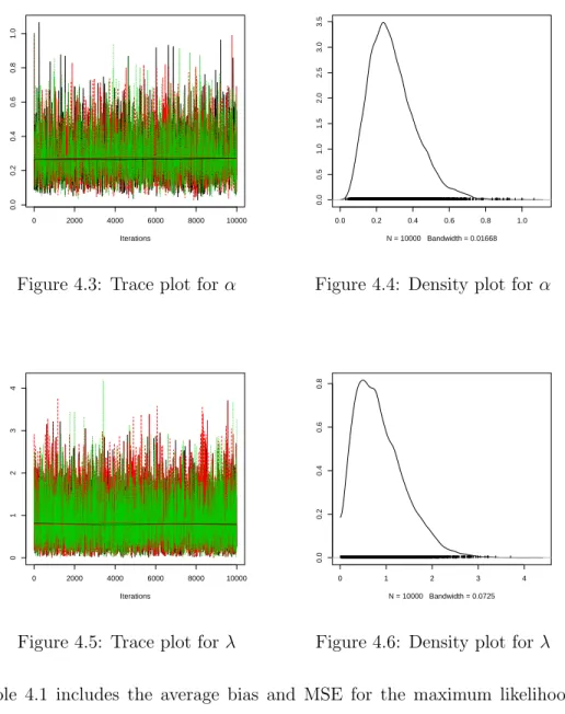
We also perform graphical diagnostics. Trace plots and density plots of the MCMC are plotted here. One can see from the trace plots that the chains have converged quite well. The density plots reﬂect the fact that the M-H algorithm uses the proposal distribution to create a mixture distribution.

(32)

0 2000 4000 6000 8000 10000 1.0 1.2 1.4 1.6 1.8 2.0 2.2 2.4 Iterations

Figure 3.3: Trace plot for α

1.0 1.5 2.0 0 1 2 3 4 N = 10000 Bandwidth = 0.0202

Figure 3.4: Density plot for α

0 2000 4000 6000 8000 10000 1.0 1.5 2.0 2.5 3.0 Iterations

Figure 3.5: Trace plot forλ

1.0 1.5 2.0 2.5 3.0 3.5 0.0 0.5 1.0 1.5 2.0 2.5 3.0 N = 10000 Bandwidth = 0.02756

Figure 3.6: Density plot for λ

likelihood estimators and the Bayes estimators under three diﬀerent loss functions for

α and λ. Average bias is listed ﬁrst and the corresponding MSE is listed second in parentheses.

n αˆM LE αˆSEL αˆW SEL αˆP L ˆλM LE λˆSEL λˆW SEL λˆP L

5 0.80 0.021 0.016 0.024 0.33 0.17 0.22 0.12 (2.85) (0.0017) (0.00093) (0.0023) (1.63) (0.75) (0.65) (0.79) 7 0.47 0.018 0.014 0.021 0.32 0.15 0.21 0.12 (0.88) (0.0010) (0.00062) (0.0013) (1.52) (0.74) (0.64) (0.78) 10 0.45 0.017 0.012 0.019 0.30 0.14 0.20 0.10 (0.42) (0.00099) (0.00051) (0.0027) (1.49) (0.039) (0.067) (0.030) Table 3.1: Average bias and MSE of estimators for αandλ

Table 3.2 includes the average interval length and coverage probability for 95% approximate conﬁdence intervals for α and λ. Average interval length is listed ﬁrst and coverage probability follows in parentheses.

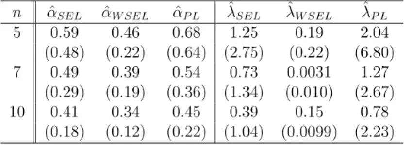
Finally, we present simulation pertaining to empirical Bayes estimation. Table 3.3 includes the average bias and MSE of the empirical Bayes estimators for αandλ.

(33)

n CIα CIλ 5 3.66 8.59 (0.984) (0.943) 7 2.36 8.49 (0.997) (0.952) 10 1.91 7.79 (0.998) (0.959)

Table 3.2: Average interval length and coverage probability for conﬁdence intervals

n αˆSEL αˆW SEL αˆP L λˆSEL λˆW SEL λˆP L

5 0.59 0.46 0.68 1.25 0.19 2.04 (0.48) (0.22) (0.64) (2.75) (0.22) (6.80) 7 0.49 0.39 0.54 0.73 0.0031 1.27 (0.29) (0.19) (0.36) (1.34) (0.010) (2.67) 10 0.41 0.34 0.45 0.39 0.15 0.78 (0.18) (0.12) (0.22) (1.04) (0.0099) (2.23)

Table 3.3: Average bias and MSE of empirical Bayes estimators forα andλ

Empirical Bayes simulation results are averages over 1000 replications. The hyper-parameters are estimated from 100 previous samples.

3.5.2 Data Analysis

To illustrate the results of this chapter, we analyze one real data set. The data is presented on page 3 of Lawless (1982). It consists of n = 11 times to breakdown of electrical insulating ﬂuid subjected to 30 kilovolts. The data, under a logarithm transformation, is2.836, 3.120, 3.045, 5.169, 4.934, 4.970, 3.018, 3.770, 5.272,

3.856, 2.046. From this data set, we extract the n= 4 upper record values 2.836,

3.120, 5.169, 5.272. Using the methods described in this chapter, we compute

the maximum likelihood estimates, as well as Bayes estimates under the squared-error, weighted squared-squared-error, and precautionary loss functions. Bayes estimates were computed with the assumption of independent gamma priors with hyper-parameters

a = c = 0.5 and b = d = 18. The estimates are in Table 3.4. In the table, the

Parameter M LE SEL W SEL P L

α 45.523 43.768 41.259 44.961

λ 13.055 17.560 17.092 17.792 Table 3.4: Estimates forαandλbased on the data

abbreviation MLE stands for maximum likelihood estimates, and the abbreviations SEL, WSEL, and PL refer to Bayes estimates under the squared error loss func-tion, the weighted squared error loss funcfunc-tion, and the precautionary loss funcfunc-tion, respectively.

(34)

After fitting the GIED, we must assess the fit. Figures 3.7 and 3.8 contain graphs of empirical and fitted survivor functions. Plotted first is the fitted survivor function using maximum likelihood estimates. Plotted second is the fitted survivor function using Bayes estimates under the weighted squared-error loss function. The weighted squared-error loss function appears to perform best of the three loss functions we consider in this situation. One can see that, while not an ideal fit, the GIED is ac-ceptable for this data set. It appears that the Bayes estimators under the weighted squared-error loss function provide a better fit than the maximum likelihood estima-tors do. 0 1 2 3 4 5 0.0 0.2 0.4 0.6 0.8 1.0 x S(x)

Figure 3.7: Empirical and ﬁtted sur-vivor function using maximum likeli-hood estimators 0 1 2 3 4 5 0.0 0.2 0.4 0.6 0.8 1.0 x S(x)

Figure 3.8: Empirical and ﬁtted sur-vivor function using Bayes estimators under the WSEL function

Finally, a two-sided Bayes probability interval for α is (28.174,61.066). A two-sided Bayes probability interval for λis (13.450,22.397).

To illustrate the prediction methods we have presented, we consider a synthetic sample ofn= 10 simulated record values. We will then predict the 11th upper record value. A randomly generated sample of upper records from a GIED with α = 1 and λ = 2 turns out to be 1.089, 3.638, 5.255, 6.093, 9.695, 31.931, 43.306,

92.525, 102.818, 4752.639. We use the M-H algorithm to generate a sample from

(3.29). Again, we assume independent gamma priors. The hyper-parameters chosen are a=c= 90 andb=d= 0.8.

The conditional median predictor, found as the median of the sample generated by the M-H algorithm, is 6491. A 95% Bayesian predictive interval for the next future record is (5777,7875).

(35)

3.6 Conclusion

The generalized inverted exponential distribution provides an excellent model for lifetime data for a variety of situations. Thus, it is important for the analyst to have reliable statistical methods to use for this distribution. We have provided both frequentist and Bayesian methods of estimating the parameters based on samples of upper record values and methods of predicting future record values. We have examined and compared the diﬀerent methods, including Bayesian methods under diﬀerent loss functions. Simulation and data analysis help to illustrate these results.

(36)

Chapter 4 Statistical Inference for the

Generalized Rayleigh Distribution

Based on Upper Record Values

4.1 Introduction

A rich class of probability distributions was introduced by Burr (1942), which includes twelve diﬀerent forms of cumulative distribution functions for modeling lifetime data. Among them, Burr Type X and Burr Type XII are the most popular ones. Several authors consider diﬀerent aspects of the Burr Type X and Burr Type XII distribu-tions. See, for example, Ahmad, Fakhry and Jaheen (1997), Jaheen (1995, 1996), Raqab (1998), Rodriguez (1977), Sartawi and Abu–Salih (1991), Surles and Padgett (1998), and Wongo (1993). For an excellent review of these two distributions the readers are refereed to Johnson et al. (1995). Recently, Surles and Padgett (2001) (see also Surles and Padgett (2004)) introduced a two-parameter Burr Type X distri-bution and correctly named it the generalized Rayleigh distridistri-bution. Note that the two-parameter generalized Rayleigh distribution is a particular case of the general-ized Weibull distribution, originally proposed by Mudholkar and Srivastava (1993). Also see Mudholkar, Srivastava and Freimer (1995). In this chapter, we call the two-parameter Burr Type X distribution the generalized Rayleigh (GR) distribution. For

α >0 and θ >0, the two-parameter GR distribution has the distribution function

F(x;α, θ) =(1₋e−(θx)2)α x_≥0, α, θ >0.

Therefore, the GR distribution has the density function

f(x;α, θ) = 2αθ2_xe−(θx)2(

1₋e−(θx)2)α−1

x_≥0, α, θ >0.

Letting λ = θ2_{, the probability density function of the two-parameter generalized}

Rayleigh distribution takes the form

(37)

The corresponding cumulative distribution function is

F(x;α, λ) =(1₋e−λx2)α x_≥0. (4.2) The survivor function takes the form

S(x;α, λ) = 1−(1−e−λx2)α x≥0, (4.3) and the corresponding hazard function is

h(x;α, λ) = 2xαλe

−λx2(

1−e−λx2)α−1

1₋(1₋e−λx2

)α x≥0. (4.4)

Here α, λ > 0 are the shape and scale parameters respectively. From now on, the two-parameter generalized Rayleigh distribution with parameters α and λ will be denoted by GR(α, λ). It is observed in Raqab and Kundu (2003) that for α≤ 1/2, the probability density function of a GR distribution is a decreasing function and it is a right skewed unimodal function for α > 1/2. Diﬀerent forms of the density functions can be found in Raqab and Kundu (2003). It is also observed that the hazard function of a GR distribution can be either bathtub shaped or an increasing function, depending on the shape parameter, α. For α < 1/2, the hazard function of a GR(α, λ) is bathtub type and for α≥ 1/2, it is increasing. Surles and Padgett (2001) showed that the two-parameter GR distribution can be used quite eﬀectively in modeling strength data and general lifetime data. Plotted below in Figure 4.1 are GR probability density functions for certain parameter settings. The solid line uses

α=.25, the dashed line usesα= 2, and the dotted line uses α= 1. All three density function plots use scale parameter λ= 1. Plotted in Figure 4.2 are hazard functions for certain parameter settings. The solid line usesα=.25, the dashed line usesα= 1, and the dotted line usesα= 4. All hazard function plots use scale parameterλ=.25.

0 1 2 3 0.0 0.5 1.0 1.5 x f(x)

Figure 4.1: GR Density Functions

0 1 2 3 0.0 0.5 1.0 1.5 2.0 2.5 x h(x)

(38)

Record values are signiﬁcant in many real life situations such as industry, weather, seismology, athletic events and economics. Chandler (1952) was the ﬁrst to introduce record values, record times and inter-record times for independent and identically distributed (iid) sequences of random variables. Feller (1966) cited some examples of record values with respect to gambling problems. The theory of record values and their distributional properties has been extensively studied in the literature. See Ahsanullah (1988, 1995), Arnold and Balakrishnan (1989), Arnold et al. (1992, 1998), and Kamps (1995) for reviews on various developments in the area of records.

The rest of this chapter is organized as follows. In Section 4.2, we derive the maximum likelihood estimators for the two parameters of a GR(α, λ) based on upper record values. In Section 4.3, we derive the Bayes estimators for the unknown param-eters under the general entropy loss function. Two-sided Bayes probability intervals are also presented. Section 4.4 presents the Bayesian predictive distribution of the future record values based on a given set of the ﬁrst n upper records. Numerical comparisons of the maximum likelihood and Bayes estimators and analysis of one data set are presented in Section 4.5. Finally, we conclude the chapter in Section 4.6.

4.2 Non-Bayesian Estimation

In this section we discuss the process of obtaining the maximum likelihood estimators of the parametersαandλbased on upper record values. Suppose we observenupper record values XU(1), XU(2), . . . , XU(n) from a sequence of independent and identically

distributed random variables from a GR(α, λ) with probability density function in (4.1). Arnold et al. (1998) give the likelihood function as

L(α, λ_|x) =f(xU(n);α, λ) n−1 ∏ i=1 f(xU(i);α, λ) 1−F(xU(i);α, λ) 0_≤xU(1)< . . . < xU(n)<∞. (4.5) Substituting (4.1) and (4.2) in (4.5), we get the likelihood function

L(α, λ|x) = 2nαnλn n ∏ i=1 xU(i)e−λ ∑n i=1x2U(i) ∏n i=1 ( 1₋e−λx2U(i) )α−1 ∏n−1 i=1 [ 1−(1−e−λx2U(i) )α]. (4.6)

The maximum likelihood estimators are the values of α and λ that maximize the likelihood function.

(39)

4.2.1 Maximum Likelihood Estimation

The log likelihood function ℓ(α, λ_|x) = logL(α, λ_|x), dropping terms that do not involve αandλ, is ℓ(α, λ|x) = n(logα+ logλ)−λ n ∑ i=1 x2U(i)+ (α−1) n ∑ i=1 log(1−e−λx2U(i)_{) (4.7)} − n−1 ∑ i=1 log[1₋(1₋e−λx2U(i) )α] .

We assume that the parametersαandλare unknown. To obtain the normal equations for the unknown parameters, we diﬀerentiate (4.7) partially with respect to α and

λ and equate to zero. The resulting equations are given below in (4.8) and (4.9), respectively. 0 = ∂ℓ ∂α = n α+ n ∑ i=1 log(1−e−λx2U(i) ) + n−1 ∑ i=1 ( 1₋e−λx2U(i) )α log(1₋e−λx2U(i) ) [ 1−(1−e−λx2U(i) )α] (4.8) 0 = ∂ℓ ∂λ = n λ− n ∑ i=1 x2U(i)+(α−1) n ∑ i=1 x2 U(i)e −λx2 U(i) ( 1−e−λx2U(i) )+α n−1 ∑ i=1 x2 U(i)e −λx2 U(i) ( 1₋e−λx2U(i) )α−1 [ 1₋(1₋e−λx2U(i) )α] (4.9) .

The solutions of the above equations are the MLEs of the parametersαandλdenoted by ˆαM LE and ˆλM LE, respectively. The equations expressed in (4.8) and (4.9) cannot

be solved analytically. Therefore, we must use iterative methods to ﬁnd numerical solutions.

4.2.2 Approximate Conﬁdence Intervals

Because the maximum likelihood estimators of the unknown parameters cannot be solved for in closed form, it is not easy to derive conﬁdence intervals for α and

λ. We must use the large sample approximation. It is known that the asymptotic distribution of the MLE ˆθis (ˆθ−θ)→N2(0, I−1(θ)), whereI−1(θ), the inverse of the

observed information matrix of the unknown parameters θ= (α, λ), is

I−1(θ) = ( −∂2ℓ(∂αα,λ|x2 ) − ∂2_ℓ₍_α,λ|x₎ ∂α∂λ −∂2ℓ∂λ∂α(α,λ|x) − ∂2_ℓ₍_α,λ_|_x₎ ∂λ2 ) −1 (α,λ)=( ˆα,ˆλ) = ( var(ˆα) cov(ˆα,λˆ) cov(ˆλ,αˆ) var(ˆλ) ) .

(40)

∂2_ℓ₍_{α, λ}_|_x₎ ∂α2 =− n α2 + n−1 ∑ i=1 ( 1−e−λx2U(i) )α[ log(1−e−λx2U(i) )]2 (( 1₋e−λx2U(i) )α −1)2 , (4.10) ∂2_ℓ₍_{α, λ}_|_x₎ ∂α∂λ = n ∑ i=1 x2 U(i) eλx2U(i)₋₁ (4.11) − n−1 ∑ i=1 x2 U(i) ( 1−e−λx2U(i) )α[( 1−e−λx2U(i) )α −αlog(1−e−λx2U(i) ) −1] ( eλx2U(i) ₋₁ ) [( 1₋e−λx2U(i) )α −1]2 , and ∂2_ℓ₍_{α, λ} |x) ∂λ2 = − n λ2 −(α−1) n ∑ i=1 x4 U(i)e λx2 U(i) ( eλx2U(i)−₁ )2 (4.12) +α n−1 ∑ i=1 x4 U(i) ( 1₋e−λx2U(i) )α( α+eλx2U(i) ( 1₋e−λx2U(i) )α −eλx2U(i) ) ( eλx2U(i)−1 )2(( 1₋e−λx2U(i) )α −1)2 .

Using this approach, we can derive 100(1₋τ)% conﬁdence intervals of the form

ˆ α±zτ /2 √ var(ˆα) and ˆ λ_±zτ /2 √ var(ˆλ).

where, zτ /2 is the upper (τ /2)th percentile of the standard normal distribution.

4.2.3 Bootstrap Conﬁdence Intervals

Here we present bootstrap conﬁdence intervals for the GR distribution. First, we will use a bootstrap method based on percentiles as presented in Efron (1982). The algorithm uses the following steps.

3. Compute the maximum likelihood estimates ˆα∗

1 and ˆλ∗1 based on the bootstrap

sample.

(41)

5. Arrange the ˆα∗

i in ascending order and obtainαU andαL, the upper and lower

limits of a 100(1₋γ)% bootstrap conﬁdence interval for α, as the γ/2 and (1₋γ/2) percentiles of the ˆα∗

i.

6. Arrange the ˆλ∗i in ascending order and obtain λU andλL, the upper and lower

limits of a 100(1−γ)% bootstrap conﬁdence interval for λ, as the γ/2 and (1−γ/2) percentiles of the ˆλ∗

i.

A second bootstrap method is based on Hall (1988). The algorithm proceeds as follows.

3. Based on the bootstrap sample, compute the maximum likelihood estimates, ˆα∗

and ˆλ∗_{, as well as the statistics}

T₁∗= √_n_(ˆ_α_∗ −αˆ) √ V ar(ˆα∗₎ and T ∗ 2 = √_n_(ˆ_λ_∗ −λˆ) √ V ar(ˆλ∗₎

where V ar(ˆλ∗_{) and} _{V ar}_(ˆ_α∗_{) are found from the observed Fisher information}

matrix.

4. Repeat steps 2 and 3N times.

5. For the values ofT1∗ andT2∗ found in step 3, let F(x) =P(Ti∗ < x), fori= 1,2

be the cumulative distribution function ofT1∗ andT2∗. Deﬁne

ˆ αt(x) = ˆα+ √ V ar(ˆα) √_n and ˆλt(x) = ˆλ+ √ V ar(ˆλ) √_n

whereV ar(ˆλ) andV ar(ˆα) are also found from the observed Fisher information matrix.

6. Approximate 100(1₋γ)% conﬁdence intervals ofαand λare given by

( ˆ αt(γ/2),αˆt(1−γ/2) ) and (ˆλt(γ/2),λˆt(1−γ/2) ) .

These bootstrap conﬁdence intervals provide an alternate to the approximate con-ﬁdence intervals derived in section 4.2.2.

Statistical Inference Based on Upper Record Values

W&M ScholarWorks

W&M ScholarWorks

Statistical Inference Based on Upper Record Values

Statistical Inference Based on Upper Record Values

f/

o

r

tO

r

s

~~

:

9

&~.

~-'

---

7

~

~

Contents

Acknowledgments

Chapter 1

Introduction

1.1

Overview and Motivation

1.2

Applications of Records

1.3

Deﬁnition of Upper and Lower Records

1.4

Distributions of Record Times and Record

Val-ues

1.4.1

Record Times

1.4.2

Record Values

Chapter 2

An Eﬃcient Algorithm for

Generating Record Values

2.1

Introduction

2.2

Algorithm for Upper Records

2.3

Algorithm for Lower Records

2.4

Illustration and Analysis

2.5

Conclusion

Chapter 3

Statistical Inference for the

Generalized Inverted Exponential

Distribution Based on Upper

Record Values

3.1

Introduction

3.2

Non-Bayesian Estimation

3.2.1

Maximum Likelihood Estimation

3.2.2

Approximate Conﬁdence Intervals

3.2.3

Bootstrap Conﬁdence Intervals

3.3

Bayesian Estimation

3.3.1

Bayes Estimators Under the General Entropy Loss

Func-tion

3.3.2

Two-Sided Bayes Probability Intervals

3.3.3

Empirical Bayes Estimation

3.4

Prediction of Future Record Values

3.4.1

Non-Bayesian Prediction

3.4.2

Bayes Prediction