Image-Based Malware Classification with Convolutional Neural Networks and Extreme Learning Machines

(1)

San Jose State University San Jose State University

SJSU ScholarWorks

Master's Projects Master's Theses and Graduate Research Fall 12-19-2019

Image-Based Malware Classification with Convolutional Neural

Networks and Extreme Learning Machines

Mugdha Jain

Follow this and additional works at: https://scholarworks.sjsu.edu/etd_projects

(2)

Image-Based Malware Classification with Convolutional Neural Networks and Extreme Learning Machines

A Project Presented to

The Faculty of the Department of Computer Science San José State University

In Partial Fulfillment

of the Requirements for the Degree Master of Science

by Mugdha Jain December 2019

(3)

(4)

The Designated Project Committee Approves the Project Titled

by Mugdha Jain

APPROVED FOR THE DEPARTMENT OF COMPUTER SCIENCE

SAN JOSÉ STATE UNIVERSITY

December 2019

Dr. Mark Stamp Department of Computer Science Dr. Thomas Austin Department of Computer Science Dr. William Andreopoulos Department of Computer Science

(5)

ABSTRACT

by Mugdha Jain

Research in the field of malware classification often relies on machine learning models that are trained on high level features, such as opcodes, function calls, and control flow graphs. Extracting such features is costly, since disassembly or code execution is generally required. In this research, we conduct experiments to train and evaluate machine learning models for malware classification, based on features that can be obtained without disassembly or execution of code. Specifically, we visualize malware samples as images and employ image analysis techniques. In this context, we focus on two machine learning models, namely, Convolutional Neural Networks (CNN) and Extreme Learning Machines (ELM). Surprisingly, we find that ELMs can

(6)

ACKNOWLEDGMENTS

I am truly grateful to have Dr. Mark Stamp as my advisor who has motivated and guided me through the research, patiently answered all my questions, encouraged me to tackle the challenging parts in this research, and always believed in me. I would also like to thank my committee members, Dr. Thomas Austin and Dr. William Andreopoulos, for their time and feedback. I am also very grateful to Fabio Di Troia, for his guidance on this project.

I am very grateful to my father for his knowledge and advice on this project and throughout the pursuit of of my Master’s degree.

(7)

TABLE OF CONTENTS CHAPTER 1 Introduction . . . 1 2 Background . . . 3 2.1 Previous Work . . . 3 3 Implementation. . . 6 3.1 Dataset . . . 6

3.1.1 Visualization of Malware Files . . . 7

3.2 Background of Classification Techniques . . . 7

3.2.1 Convolutional Neural Networks . . . 7

3.2.2 Extreme Learning Machine . . . 10

4 Results and Analysis . . . 14

4.1 CNN . . . 14

4.1.1 1C: Architectures with 1 Convolutional Layer . . . 14

4.1.2 2C: Architectures with 2 Convolutional Layers . . . 19

4.2 ELM . . . 25

4.2.1 100% MLP Input Activation . . . 25

4.2.2 50% MLP and 50% RBF Input Activation . . . 26

4.2.3 100% RBF Input Activation . . . 28

4.2.4 Cross Validation for Checking Stability . . . 29

4.2.5 Ensemble Classifier with Majority Vote . . . 30

(8)

4.2.7 1-Dimensional Input . . . 33

5 Conclusion and Future Work . . . 39

5.1 Future Work . . . 40

LIST OF REFERENCES . . . 42

APPENDIX Additional Results . . . 45

A.1 CNN: 2 Convolutional Layers . . . 45

A.1.1 Model 1 . . . 45 A.1.2 Model 2 . . . 45 A.1.3 Model 3 . . . 45 A.1.4 Model 4 . . . 45 A.1.5 Model 5 . . . 47 A.1.6 Model 6 . . . 47 A.1.7 Model 7 . . . 47 A.2 ELM . . . 50

(9)

LIST OF TABLES

1 Accuracies for CNN models with 1 convolutional layer . . . 15 2 Accuracies for CNN models with 2 convolution layers . . . 20 3 Standard deviation across 50 ELMs with𝛼 = 1.0 . . . 27

(10)

LIST OF FIGURES 1 Class Distribution . . . 6 2 Adialer.C samples . . . 7 3 Dialplatform.B samples . . . 8 4 Dontovo.A samples . . . 8 5 CNN Architecture . . . 9 6 Convolutional Layer . . . 10 7 Max Pooling . . . 10

8 Architecture of ELM Model . . . 11

9 Class-wise accuracies for 1C (32×32 images and 32 filters) . . . . 16

13 Class-wise accuracies for 1C (128×128 images and 32 filters) . . 19

14 Swizzor.gen!I and Swizzor.gen!E . . . 19

15 Autorun.K and Yuner.A . . . 20

16 Confusion matrix for CNN model with 128×128 images and 32 filters 21 17 Class-wise accuracies for 1C (128×128 images and 64 filters) . . 22

18 Class-wise accuracies for 2C (32×32 images and (64,64) filters) . 23 19 Class-wise accuracies for 2C (64×64 images and (64, 32) filters) . 23 20 Class-wise accuracies for 2C (128×128 images and (32, 64) filters) 25 21 Average accuracy of 50 ELMs (𝛼= 1.0) . . . 26

(11)

22 Average accuracy of 50 ELMs (𝛼= 0.5) . . . 28

23 Average accuracy of 50 ELMs (𝛼= 0.0) . . . 29

24 Average accuracy across 10 folds (64×64 images) . . . 30

25 Ensemble Classifier Accuracy (64×64 images) . . . 31

26 Cross validation of ensemble classifier (64×64 images) . . . 32

27 Fully connected vs. dropout . . . 32

28 Average accuracy for fully connected vs dropout ELM (64×64 images) . . . 33

29 Ensemble accuracy for fully connected vs dropout ELM (64×64 images) . . . 34

30 Average ensemble accuracy vs. number of neurons (512×1 images 35 31 Average ensemble accuracy with varying input dimension . . . . 36

32 Cross validation of dropout ELM (512×1 images) . . . 37

33 Weighted ELM Accuracy (1024×1 images) . . . 38

34 Class-wise F1 scores for CNN and ELM . . . 40

A.35 Class-wise accuracies (32×32 images, 2 convolutional layers with 32, 32 filters respectively) . . . 45

A.39 Class-wise accuracies (64×64 images, 2 convolutional layers with 32, 64 filters respectively)) . . . 48

(12)

A.41 Class-wise accuracies (128×128 images, 2 convolutional layers

with 32, 32 filters respectively) . . . 49 A.42 Training/Testing Accuracy vs No. of Neurons (50 ELMs, 𝛼= 1.0) 50 A.43 Training Time (activation function = ’relu’) . . . 51 A.44 Cross Validation: Average accuracy across 10 folds (32×32 images) 51 A.45 Cross validation of ensemble classifier (32×32 images) . . . 52 A.46 Average accuracy for fully connected vs dropout ELM (32×32

images) . . . 53 A.47 Ensemble accuracy for fully connected vs dropout ELM (32×32

images) . . . 53 A.48 Average ensemble accuracy over 10 folds (512×1 images, 512

neurons) . . . 54 A.49 Average ensemble accuracy over 10 folds (512×1 images, 1024

neurons) . . . 54 A.50 Average ensemble accuracy over 10 folds (512×1 images, 2048

neurons) . . . 55 A.51 Training time for CNN and ELM . . . 55

(13)

CHAPTER 1 Introduction

Malware is any program that is developed to disrupt computer systems without the owner’s knowledge. In the third quarter of 2018, at least 239 million new malware variants and samples were detected [1] and 669 million new malware variants were detected in the previous year. The large quantity of malware detected in 2017 was up by 80.1% from 2016 [2]. Thus, malware detection is a critical task in computer security.

Malware detection techniques can be broadly categorized into anomaly-based and signature-based. Although these methods are commonly used to develop antivirus software, each has certain disadvantages. Obfuscation can be used to defeat signature-based detection [3], while anomaly-signature-based methods are computationally more expensive and also have higher false flagging [4]. Malware detection techniques based on machine learning models can overcome these weaknesses.

Successful models have been developed using machine learning with high-level features like opcode sequences, function calls, or control flow graphs [5, 6, 7]. However, extracting such high-level features can be difficult and time consuming. To overcome these issues it is better to directly use byte data of the malware executables [5]. The extraction of these features can be done without performing disassembly of the code and without executing the code.

In this research, we use the MalImg dataset [8] wherein malware files have been converted into images. The byte values of the malware executable are treated as grayscale intensity values for pixels in the image [8].

The primary focus of our research is to compare the classification performance of Convolutional Neural Networks (CNN) and Extreme Learning Machines (ELM) for the classification of malware images.

(14)

CNNs have been studied extensively and have shown to perform well in im-age classification tasks [9]. Extreme Learning Machines (ELM) are a less explored technique but can deliver comparable performance on many classification tasks. In addition, compared to models trained with back-propagation algorithm, ELMs are computationally more efficient [10]. This makes ELMs attractive for malware classifi-cation, particularly when considering the large and growing volume of new malware and their variants.

The experiments are conducted by training CNN and ELM models on the MalImg dataset [8]. Extensive parameter tuning is also conducted to optimize the performance of each model. To address the instability issues because of random assignment of input layer weights in ELMs, we explore an ensemble approach [11].

The remainder of this paper is organized as follows. Chapter 2 discusses previous work related to this research problem. In Chapter 3 we give a broad summary of the malware families and the dataset used in the research. Also, we briefly discuss the machine learning techniques that are used in the experiments. In Chapter 4, we present and analyze the results of our experiments. Finally, in Chapter 5, we summarize this research and discuss possible avenues for future work.

(15)

CHAPTER 2 Background

With new variants of malware being released every year, computer security has become an important field [6]. To identify new and unknown malware quickly, malware detection techniques must also be constantly upgraded. Fast and accurate detection of malware has become important for computer and network security [6].

Malware classification can be based on static analysis or behavioral analysis. Static features are extracted from malware files while in behavioral analysis, dynamic features are extracted during code execution. Some examples of static features are byte sequences directly taken from malware files, calls to external libraries [12], sequences of API calls [13] and opcode features [14]. On the other hand, dynamic features could be based on resource usage by the system or frequency of calls to kernel functions.

Malware detection techniques based on signatures are quite popular. However, their disadvantage is that new malware can always be created with new signatures thus avoiding detection. Code obfuscation can also be utilized by malware creators to defeat signature based models. In anomaly-based techniques, profiles that describe typical characteristics of a system are used to classify malware as normal or abnormal. However this method frequently produces false positives [4]. Machine learning based models can overcome some of these weaknesses.

The following section describes a few malware detection and classification tech-niques described in literature.

2.1 Previous Work

An opcode based approach for classification of malware and benign software is described in [7]. They use a tf-idf (Term Frequency Inverse Document Frequency) like approach to convert malware files into feature vectors, where each feature is a measure of the relevance or weight of that opcode based on the frequency of its

(16)

occurrence in that file and other files. Although they obtained satisfactory results, this technique requires disassembly of malware to extract opcodes. Another opcode based technique is proposed in [6], using a graph representing pairs of consecutive opcodes. A feature vector is constructed from this graph by embedding this graph into a vector space. Although they obtain good results, the technique used to obtain the embedding converges slowly.

In [15], the authors use frequencies of byte substrings in malware files as features. Instead of considering the whole file, only specific sections of the file are considered. Their technique achieves good results in detecting new malware.

The previous method is improved upon in [16], where the authors propose a method of using the most important𝑛-grams of bytes in each malware executable as features of that file. They use𝑛-grams treated as binary attributes indicating their presence/absence. The important 𝑛-grams are chosen on the basis of Information Gain (IG) and various learning algorithms are trained on these features to compare classification performance. The method proposed in [17], is a signature based method and also uses 𝑛-grams. They achieve best results for 4-grams.

In [18], the authors propose a technique to convert malware into audio signals. Each byte of the malware is mapped to a musical note in the MIDI schema. Thus, byte data is converted into music. Audio features such as zero crossings rate, MFCC etc. are extracted to train machine learning models. This technique achieves an accuracy of above 90%.

ELMs have been introduced to malware detection on the Android platform in [19]. Static features were used for training ELM achieving good accuracy on classification of malware. In [20], the authors compare and contrast the performance of ELM with other models on two different malware datasets showing that ELMs achieved highest accuracy in their study.

(17)

An interesting variation of ELM architecture is proposed in [21]. Typically, ELMs have only one hidden layer. Here, the authors propose a partially connected layer after the input layer, followed by a fully connected hidden layer next. Finally, they use an ensemble of two layer ELMs for malware assessment, obtaining highly accurate results.

In [8], the authors propose conversion of malware into images which are grayscale. They observe that images of the same family are close to each other in appearance. They trained models on GIST descriptors and achieved an accuracy of 98%. This approach does not require disassembly or execution.

This research is highly motivated by the work in [8]. Inter-family differences are more pronounced as compared to intra-family appearances in the malware images. Moreover, if malicious code is re-used to create variants, the images of the new variants would retain visual characteristics of the original malware. In contrast to their technique, we propose the use of CNNs and ELMs trained directly on pixel data, rather than GIST descriptors, as discussed in more detail in Chapter 3.

(18)

CHAPTER 3 Implementation

In this chapter, we give a broad summary of the malware families and the dataset used in the research. Also, we briefly discuss the machine learning techniques that were used in the experiments.

3.1 Dataset

The MalImg dataset described in [8] is used in our experiments. The dataset comprises of 9342 grayscale images belonging to 25 different malware families. The dataset is highly imbalanced and five familiesAllaple.A,Allaple.L,Yuner.A,VB.AT,

Fakeranand Instanaccess make up two thirds of the dataset. Figure 1 shows the number of images present in each family.

(19)

3.1.1 Visualization of Malware Files

In [8], the authors convert malware into images. The malware file is read byte-by-byte and mapped to pixels values in the range [0,255]. 0 implies black and 255 implies white. This list of pixel values is then converted into a two dimensional image. The authors have defined a specific image width for specific ranges of file sizes. Thus the image dimensions completely depend on the size of the malware file.

The following figures show three different samples belonging to three malware families. Figure 2 shows samples of Adialer.C family. Figure 3 shows samples of

Dialplatform.B family. Figure 4 shows samples of Dontovo.A family. These images show the visual similarity within a particular malware family and how they differ from other malware families.

Figure 2: Adialer.C samples

3.2 Background of Classification Techniques

In this section, we describe the machine learning models, CNNs and ELMs, used in the experiments.

3.2.1 Convolutional Neural Networks

Convolutional Neural Networks work very similar to how humans recognize images. They are based on the work described in [22], where studies were conducted to understand how mammals perceive the world visually. The study determined that cells in the brain activate based on visual stimuli such as edges and shapes. CNNs are

(20)

Figure 3: Dialplatform.B samples

Figure 4: Dontovo.A samples

popular deep learning models most commonly used for image classification problems and are essentially a feed-forward neural network. Figure 5 shows the architecture of a simple CNN. For this research, CNNs were implemented using Keras [23]. CNNs usually have the following three types of layers:

(21)

2. convolutional layer 3. pooling layer

Figure 5: CNN Architecture

3.2.1.1 Convolutional Layer

The convolutional layer is a fundamental part of CNNs. Convolution is a mathematical combination of two functions. This layer combines the input with a filter. This operation produces a feature map [24]. Figure 6 shows how the convolutional layer performs a matrix multiplication of the filter with the input. Several filters of different sizes can be used. Each filter moves over the input until the entirety of the input is covered. This movement of the filter can be controlled using stride, which specifies how much the filter moves in each step, from left to right and top to bottom. The output of the convolutional layer is all the feature maps produced across all filters. In Figure 6, the filter moves with a stride of 1, covering the input image in 4 moves.

3.2.1.2 Pooling Layer

A convolutional layer is followed by a pooling layer. This layer downsamples the output of the convolutional layer [25]. This reduction directly translates to a decrease in the number of computations and hence a reduction in training time. There are several techniques for implementing pooling. For this research we use max pooling.

(22)

Figure 6: Convolutional Layer

Figure 7 shows how max pooling works to downsample input. The input is first divided into sections without overlap. The maximum value within each section is retained for the next set of computations.

Figure 7: Max Pooling 3.2.2 Extreme Learning Machine

ELMs were first proposed in [26]. An ELM has a simple architecture with the input layer connected to the hidden layer, and the hidden layer connected to the output layer. An ELM usually has only one hidden layer. The weights and biases matrices between the input layer and the hidden layer are assigned arbitrarily [10]. These are only calculated once unlike back-propagation algorithms which go back and forth to repeatedly adjust weights. This one time calculation makes ELMs extremely

(23)

fast for training [10].

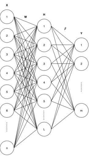
Figure 8: Architecture of ELM Model

Consider the ELM architecture shown in Figure 8 with 𝑋 denoting the input layer, 𝐻 denoting the hidden layer and 𝑌 denoting the output layer. Consider 𝑁 arbitrary distinct samples (𝑥𝑖, 𝑦𝑖) for 𝑖 = 1,2, . . . , 𝑁, where 𝑥𝑖 is an input sample

with [𝑥𝑖1, 𝑥𝑖2, . . . 𝑥𝑖𝑛]𝑇 features and 𝑦𝑖 = [𝑦𝑖1, 𝑦𝑖2, . . . 𝑦𝑖𝑚]𝑇 denote the output labels.

Then, the input and output for the ELM can be shown as 𝑋 = [𝑥1, 𝑥2, . . . , 𝑥𝑛]𝑇 and

𝑌 = [𝑦1, 𝑦2, . . . , 𝑦𝑚]𝑇 respectively, where 𝑇 indicates the transposition operation.

Suppose the hidden layer 𝐻 has 𝐿 neurons. Let the activation function of the hidden layer be𝑔(𝑥).

(24)

The ELM model selects the weight matrix 𝑊 of the input layer 𝑋 to the hidden layer𝐻randomly. Let𝑊 = [𝑤1, 𝑤2, . . . , 𝑤𝐿]𝑇. The ELM also selects the bias matrix𝐵

of the input layer𝑋 to the hidden layer𝐻 randomly. Let𝐵 = [𝑏1, 𝑏2, . . . , 𝑏𝐿]𝑇. During

the training phase, both 𝑊 and 𝐵 remain unchanged. Hence, after 𝑊 and𝐵 have been chosen, the value of the hidden layer 𝐻 can be calculated as

𝐻 =𝑔(𝑊 𝑋+𝐵).

The output 𝑌 can then be calculated using Equation 1.

𝑌 =𝐻𝛽 (1)

In Equation 1, 𝛽= [𝛽1, 𝛽2, . . . , 𝛽𝐿]𝑇 is the weight matrix between hidden layer 𝐻

and output layer 𝑌. The values of the weights of the hidden layer, that is, 𝛽, can be computed in one single operation using 𝐻†, the Moore-Penrose generalization inverse

of 𝐻, resulting in the solution with the least error to predict target 𝑌 as

𝛽=𝐻†𝑌

The only parameter an ELM calculates is 𝛽. Given that 𝑌 is the target, a unique solution of the system with least squared error can be found using Moore-Penrose generalized inverse. 𝐻† is the Moore-Penrose generalization inverse of 𝐻 and can

be calculated as 𝐻† = ⎧ ⎪ ⎪ ⎪ ⎨ ⎪ ⎪ ⎪ ⎩ (𝐻𝑇_𝐻₎−1_𝐻𝑇 _if _𝐻𝑇_𝐻 _{is nonsingular} 𝐻𝑇₍_𝐻𝐻𝑇₎−1 _if _𝐻𝐻𝑇 _{is nonsingular}

After calculating 𝛽, the training phase ends. For each test sample𝑥, the output 𝑌 can be calculated as

𝑌 =𝑔(𝑊 𝑥+𝐵)𝛽

For this project we used the python implementation of ELMs in [27] which describes the input activations as a weighted combination of the multi layer perceptron

(25)

(MLP) output and the radial basis function (RBF) kernel output, where

input_activation =𝛼mlp_activation+ (1−𝛼)rbf_activation

mlp_activation(𝑥) =𝑊 𝑥+𝐵

rbf_activation(𝑥) = rbf_width||𝑥−center||

center

Here, the mlp_activation is the multilayer perceptron input activation,

rbf_activationis the radial basis function input activation, 𝑊 and𝐵 are randomly

chosen and follow normal distribution, center is taken uniformly from the bounding

box hyper-rectangle of the inputs and center = max(|| 𝑥−𝑐 ||)/√2×n_centers,

where n_centers is the number of cluster centers. The parameter 𝛼 is called the

mixing parameter and can have a value between 0.0 (100% RBF input activation) and 1.0 (100% MLP input activation).

Thus, the value of the hidden layer 𝐻 is calculated as described in Equation 2. Finally the output 𝑌 is calculated by substituting Equation 2 in Equation 1.

(26)

CHAPTER 4 Results and Analysis

In this chapter, we discuss the results and analysis of the experiments performed by training CNNs and ELMs on the MalImg dataset. The chapter has two sections discussing the results of experiments conducted for each model.

4.1 CNN

This section describes CNN experiments and their results. Each CNN model was trained for 50 epochs and with therelu activation function. Various CNN architectures with different combinations of convolution, pooling and dense (fully-connected) layers along with hyperparameter tuning with different input image size, batch size, number of filters, filter size and pooling size were tested.

4.1.1 1C: Architectures with 1 Convolutional Layer

This section describes the experiments conducted with CNN models with 1 convolutional layer. These models were trained on combinations of 3 different input image sizes (32×32 pixels, 64×64 pixels and 128×128pixels) and number of filters (32 and 64). Each CNN model has a layer of size 2×2, a fully connected layer with 128 neurons and an output layer with 25 neurons corresponding to each class with softmax activation. For each experiment, we describe the architecture of the

CNN, followed by the overall accuracy of the model and accuracies per class. Table 1 summarizes these results.

4.1.1.1 CNN: Image Size 32×32 pixels

The first model consists of input image size of 32×32 pixels and 1 convolutional layer with 32 filter maps of size 3×3. This model does not perform very well, achieving an overall accuracy of 84%. The class-wise accuracies are summarized in Figure 9. The images in the original dataset vary in dimensions and are very large in comparison to the resized 32×32 input. The resizing also disturbs the aspect ratio of the original

(27)

Table 1: Accuracies for CNN models with 1 convolutional layer Image Size Filters Accuracy

32×32 32 0.8400 32×32 64 0.8467 64×64 32 0.9340 64×64 64 0.9245 128×128 32 0.9630 128×128 64 0.9589

image, hence, this CNN seems to perform poorly.

Increasing the number of filters to 64 and leaving the other parameters unchanged increases the classification accuracy marginally to 84.67%. More filters imply more feature maps, which means the CNN is identifying more features to classify the images. But in this case, the increase in performance is not justified considering the cost of computation with respect to more filters. The class-wise accuracies are summarized in Figure 10. The second model with 64 filters also fails to predict any images from

Swizzor.gen!I family. Overall, the second model achieves an accuracy of 90% or greater for 15 classes as compared to 12 classes for the first model.

The models described in this section are trained on images of size 64×64 pixels. The remaining parameters remain the same as in Section 4.1.1.1. Even with 32 filters, the CNN achieves an accuracy of 93.40%. This is a significant improvement over the previous experiments. Clearly, increasing the image size affects the model performance significantly. The class-wise accuracies are summarized in Figure 11. Surprisingly, increasing the number of filters to 64 drops the accuracy to 92.45%. The class-wise accuracies for this configuration is summarized in Figure 12.

(28)

Figure 9: Class-wise accuracies for 1C (32×32 images and 32 filters)

overall accuracy, the two models perform significantly better than the models in Section 4.1.1.1. However, both models fail to predict any images from Autorun.K

(29)

second model also fails to predict images of Malex.gen!Jfamily. Both families are

minor classes in the dataset with approximately 100 images each.

(30)

Training the CNNs on images of size 128×128 pixels with only 32 filters results in an accuracy of 96.3%. Based on overall accuracy, this is the best performing CNN model in our research. The class-wise accuracies are summarized in Figure 13 and its confusion matrix is shown in Figure 16. This model is able to achieve an accuracy of above 90% for 16 out of the 25 classes in the dataset. Only one family, Autorun.K

has an accuracy below 50%.

The confusion matrix in Figure 16 also shows the malware families that are fre-quently misclassified. For instance, 5 out of 12 samples of the family Swizzor.gen!I

are misclassified as belonging to Swizzor.gen!E. The visual similarity between

mal-ware images from these families can be seen in Figure 14. A similar behavior is observed for samples of Autorun.K where all have been misclassified into the family

Yuner.A. The visual similarity between these two families is shown in Figure 15. Increasing the number of filters to 64 brings down the accuracy to 95.89% showing that increasing number of filters does not always give the desired or expected results. This model predicts 4 families with below 50% accuracy as compared to only 1 family in the first model. The class-wise accuracies are summarized in Figure 17.

For all 3 image sizes, increasing the number of filters has a minimal effect on the CNN performance. This could be attributed to the fact that images in the dataset are in grayscale with only 1 channel. Images in color have 3 channels for red, blue and green implying that more filters actually translates to learning more features. There is definite and steady increase in accuracy when increasing the size of the input images lending merit to the fact that different input image size seems to distort patterns within the image that the CNN utilizes for classification. For example, the family

Autorun.Kis predicted with 100% accuracy for all models with input size 32×32 but

(31)

Figure 14: Swizzor.gen!I and Swizzor.gen!E

4.1.2 2C: Architectures with 2 Convolutional Layers

This section describes the experiments conducted with CNN models with 2 convolutional layers. These models were trained on combinations of 3 different input image sizes (32×32 pixels, 64×64 pixels and 128×128 pixels) and number of filters

(32)

Figure 15: Autorun.K and Yuner.A

(32 and 64). Each CNN has a max-pooling layer of size 2×2, a fully connected layer with 128 neurons and an output layer with 25 neurons corresponding to each class with softmax activation. For each experiment, we describe the architecture of the

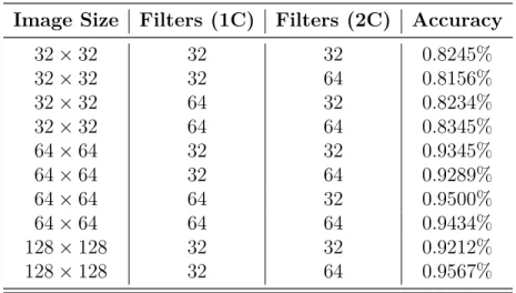
CNN, followed by the overall accuracy of the model and accuracies per class. Table 2 summarizes these results. Additional experiment results can be found in Appendix A.

Table 2: Accuracies for CNN models with 2 convolution layers Image Size Filters (1C) Filters (2C) Accuracy

32×32 32 32 0.8245% 32×32 32 64 0.8156% 32×32 64 32 0.8234% 32×32 64 64 0.8345% 64×64 32 32 0.9345% 64×64 32 64 0.9289% 64×64 64 32 0.9500% 64×64 64 64 0.9434% 128×128 32 32 0.9212% 128×128 32 64 0.9567%

(33)

Figure 16: Confusion matrix for CNN model with 128×128 images and 32 filters

This model consists of input image size of 32×32 pixels and 2 convolutional layers with 64 filter maps each of size 3×3. This two convolutional layer architecture does not perform very well, achieving an overall accuracy of 83.4%. The class-wise accuracies are summarized in Figure 18.

Convolutional layers need not be applied to only input data, that is, raw pixel values. They can also be applied to the output of other convolutional layers. This

(34)

stacking of convolutional layers allows a hierarchical decomposition of the input. The filters that operate directly on the raw pixel values will learn to extract low-level features, such as lines or edges. The filters that operate on the output of the first few layers may extract features that are combinations of lower-level features, such as features that comprise multiple lines to express shapes.

The expectation from a complex architecture is for it to learn local as well as global features, but the drawback of having multiple convolutional layers is the loss in speed, since this model performs several more computations. Surprisingly, the 2 convolutional layer model performs marginally worse than the 1 convolutional layer models in Section 4.1.1.1.

This model consists of input image size of 64×64 pixels, 2 convolutional layers with 64 and 32 filter maps of size 3×3 respectively. This model achieved an overall accuracy of 95%, significantly better that the previous 2 layer architecture and better

(35)

Figure 18: Class-wise accuracies for 2C (32×32 images and (64,64) filters)

than the CNNs in Section 4.1.1.2. The class-wise accuracies are summarized in Figure 19.

(36)

This model consists of input image size of 128×128 pixels and 2 convolutional layers with 32 and 64 filter maps of size 3×3 respectively. This model achieved an overall accuracy of 95.67%, only marginally better than previous 2 layer architectures. The class-wise accuracies are summarized in Figure 20.

The 2 convolutional layer models did not show a significant improvement over 1 convolutional layer modes in Section 4.1.1. This is a surprising result considering that more complex architectures were expected to perform better. The five families

Allaple.A, Allaple.L, Yuner.A, VB.AT, Fakeran and Instanaccess have already achieved an accuracy of close to 100% with 1-convolutional layer. Any improvement beyond this could only come from increasing the accuracy of the smaller classes. Since these 5 classes make up two-thirds of the dataset, this imbalance could have prevented the 2 convolutional layer models from performing better. The marginal improvement in performance also comes at the cost of training time, because the complex CNN architectures in Section 4.1.2 take more time to train. The results in Section 4.1.1 and Section 4.1.2 also demonstrate that an image size of 32×32 is not the optimum input size to train the CNN as there is a significant loss of information during the resizing operation. Better results are consistently obtained for image sizes 64×64 and 128×128. We also see that for this dataset, increasing the number of filters does not always result in better performance. It has a marginal positive or negative effect and a likely explanation is that the dataset consists of grayscale images with only 1 channel. With a filter size of 3×3, there is not enough information to differentiate with more filters.

(37)

Figure 20: Class-wise accuracies for 2C (128×128 images and (32, 64) filters)

4.2 ELM

This section describes ELM experiments and results. As with CNNs, we test various ELM architectures by experimenting with the number of neurons in the hidden layer and activation functions. We also experiment with fully connected hidden layers and hidden layers with dropout. For each combination of parameters, we train and test 50 ELMs and evaluate the performance by looking at the average accuracy. 4.2.1 100% MLP Input Activation

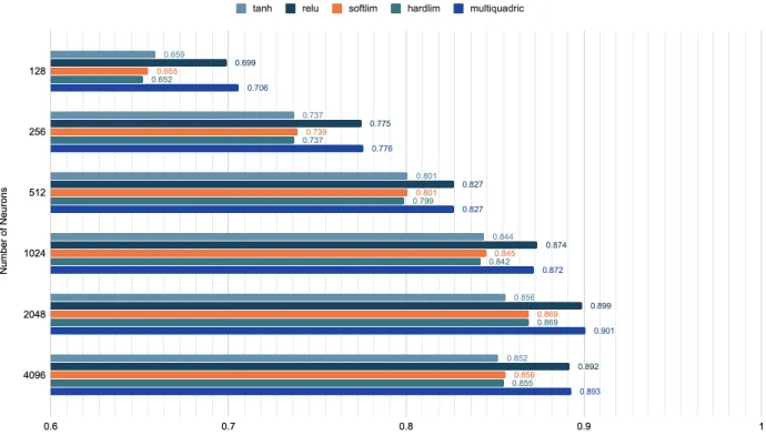
50 ELMs were trained on image size 64×64 pixels with𝛼= 1.0 (100% MLP input activation). Activation functions (tanh, relu, softlim, hardlim, multiquadric ) with number of neurons (128, 256, 512, 1024, 2048, 4096). Figure 21 shows the average accuracies over 50 ELMs with the specified parameters. Despite randomly chosen 𝑊 and𝐵 (weights and biases), the ELMs perform quite consistently as evidenced by the standard deviations in Table 3.

(38)

Figure 21: Average accuracy of 50 ELMs (𝛼= 1.0)

tanh, softlim and hardlim as the number of neurons increases. Moreover, the average accuracies increase with more neurons in the hidden layer until a marginal drop from 2048 to 4096 neurons. At 4096 neurons, the training accuracy reaches 1.00 across all activation functions as seen in Appendix A. This drop in accuracy, along with the trend in training accuracy points towards ELMs overfitting.

4.2.2 50% MLP and 50% RBF Input Activation

50 ELMs were trained on image size 64×64 pixels with 𝛼 = 0.5 (50% MLP and 50% RBF input activation). Activation functions (tanh, relu, softlim, hardlim, multiquadric ) with number of neurons (128, 256, 512, 1024, 2048, 4096). Figure 22 shows the average accuracies across these 50 ELMs with the specified parameters.

Again, relu and multiquadric outperform other activation functions, with accu-racies increasing with the number of neurons. There is a significant jump in the

(39)

Table 3: Standard deviation across 50 ELMs with 𝛼= 1.0

Neurons Activation Standard

Deviation tanh 0.014 relu 0.013 128 softlim 0.016 hardlim 0.016 multiquadric 0.012 tanh 0.013 relu 0.011 256 softlim 0.015 hardlim 0.011 multiquadric 0.011 tanh 0.01 relu 0.008 512 softlim 0.009 hardlim 0.008 multiquadric 0.007 tanh 0.008 relu 0.007 1024 softlim 0.009 hardlim 0.007 multiquadric 0.008 tanh 0.096 relu 0.007 2048 softlim 0.009 hardlim 0.008 multiquadric 0.005 tanh 0.007 relu 0.008 4096 softlim 0.009 hardlim 0.007 multiquadric 0.006

performance of tanh, softlim and hardlim as compared to Section 4.2.1, however relu and multiquadric remain the same.

(40)

4.2.3 100% RBF Input Activation

50 ELMs were trained on image size 64×64 pixels with 𝛼 = 0.0 (100% RBF input activation). Activation functions (tanh, relu, softlim, hardlim,multiquadric ) with number of neurons (128, 256, 512, 1024). Figure 23 shows the average accuracies across these 50 ELMs with the specified parameters.

Again, relu and multiquadric outperform other activation functions, with ac-curacies increasing with the number of neurons. There is a significant drop in the performance of tanh, softlim and hardlim which show no improvement with increas-ing number of neurons. Relu and multiquadric perform the same as compared to Section 4.2.1 and Section 4.2.2.

Based on these experiments, the following parameters are chosen for training ELMs (unless specified otherwise):

(41)

1. Relu activation function

2. 𝛼= 1.0: This value is chosen because of fastest training time; calculation of rbf input activation is computationally heavy

3. Number of neurons: 1024

4.2.4 Cross Validation for Checking Stability

To check the stability of ELMs and reduce any bias, cross validation was performed on 10 folds of the dataset. For this an 85%−15% split of the data was taken class-wise.The results can be seen in Figure 24. The parameters of this models are:

1. Image size = 64×64 2. No. of neurons = 1024 3. Activation function = relu

(42)

The accuracy remains stable across the ten folds with the maximum and minimum accuracy as 87.8% and 87.2% respectively. The consistent performance of ELMs is surprising considering:

• randomly chosen 𝑊 and 𝐵

• lack of back-propagation to adjust weights

Figure 24: Average accuracy across 10 folds (64×64 images)

4.2.5 Ensemble Classifier with Majority Vote

Ensemble learning helps improve machine learning results by combining several models into one predictive model in order to decrease variance and bias and thus improving predictions. For this research, we use the simple technique of majority vote to build the ensemble classifier. 50 individual ELM classifiers are combined by taking a simple majority vote of their decisions. For any given instance, the class chosen by most number of classifiers is the ensemble decision.

Figure 25 shows that with increasing number of neurons, ensemble accuracy consistently increases. The ensemble classifier always performs better than the individual ELMs.

(43)

Figure 26 show cross validation of the ensemble technique on 10 folds of the data. The graph shows the average accuracy of 50 ELMs vs the accuracy achieved by the ELM Ensemble Classifier for that fold. Ensemble of ELMs consistently achieves better result for different input image sizes. Additional results with input image size 32×32 are included in Appendix A.

Figure 25: Ensemble Classifier Accuracy (64×64 images)

4.2.6 Fully Connected ELM vs. ELM with Dropout

Fully connected layer implies each neuron in the hidden layer is connected to all nodes in the input layer. Therefore it increases the probability of the neurons in the hidden layer developing codependency on each other, leading to overfitting. Dropout is one of the techniques to reduce overfitting. In dropout, some of the neurons are disregarded. Traditionally in dropout, only a small number of neurons are dropped randomly [28]. Figure 27 shows that neurons marked with "×" are dropped.

(44)

Figure 26: Cross validation of ensemble classifier (64×64 images)

Figure 27: Fully connected vs. dropout

we implement a simple algorithm that connects each neuron in the hidden layer to only a few input nodes taken sequentially. This technique is very different from how dropout is usually implemented. Here, neurons to be dropped are not chosen randomly. Moreover, a very large percentage of connections is being lost. In our experiments, every neuron in the hidden layer is only connected to 4 input nodes, instead of all

(45)

input nodes. This can be visualized as a sliding window of 4 input nodes moving over the input layer such that every input node is connected to atleast 1 neuron in the hidden layer. This ensures that hidden layer neurons have minimum codependency on each other. Figure 28 shows average accuracies across 50 ELMs trained with and without dropout over 10 folds of the data. Dropout ELMs consistently perform better than fully connected traditional ELMs. Figure 29 shows the average accuracy of the corresponding ensemble classifiers, that is, ensemble classifier built from fully connected ELM and ensemble classifier built from dropout ELMs. Again, the ensemble with dropout consistently performs better than fully connected ensemble by about 2%.

Figure 28: Average accuracy for fully connected vs dropout ELM (64×64 images)

4.2.7 1-Dimensional Input

Malware executables are essentially a sequence of bytes. When these are converted to images, sequential patterns present in the executables are lost because the image dimensions vary according to the size of the malware [8]. The 1-dimensional patterns

(46)

Figure 29: Ensemble accuracy for fully connected vs dropout ELM (64×64 images)

existing in the original malware file, are lost during their conversion into 2-dimensional space (images).

To preserve these sequential patterns, we propose a different technique for ELM inputs. The original image of malware from the dataset is read as a 1-dimensional vector, taking pixels from left to right and going top to bottom. Since the images in the dataset are of varying dimensions, the 1-dimensional vector also differs in length.Let this length be𝑇. Let 𝑁 be the desired length of the 1-dimensional vector.

If𝑇 is divisible by𝑁, then in the original vector we take _𝑁𝑇 elements consecutively and average their values. If 𝑇 is not divisible by𝑁, we pad the original vector with zeros at the end in order to make 𝑇 divisible by 𝑁. The result is a 1-dimensional input vector of dimensions 𝑁 ×1.

(47)

4.2.7.1 No. of Neurons vs. Average Ensemble Accuracy

For this experiment 3 ensemble classifiers with 50 dropout ELMs each were trained on ten folds of the dataset. The input to each ELM was a vector of dimensions 512×1. ELMs were trained with 512, 1024 and 2048 neurons respectively, with 𝛼= 1.0. Each ELM used therelu activation function. Each ensemble classifier was tested on 10 folds of the data. Figure 30 shows the average ensemble classifier accuracy over the ten folds. Additional experiment results can be found in Appendix A. The best accuracy is achieved for ELMs with 1024 neurons. However, increasing the number of neurons has a marginal effect on the overall performance of the ELM.

Figure 30: Average ensemble accuracy vs. number of neurons (512×1 images

4.2.7.2 Input Dimension vs Average Ensemble Accuracy

For this experiment, ensemble classifiers were built from dropout ELMs trained on 3 input dimensions of size 512×1, 1024×1 and 4096×1, with 𝛼= 1.0 and relu activation function. Figure 31 shows the average accuracy of the ensemble classifiers over ten folds of the data. Increasing the dimensionality of the input to 4096×1 has a marginal effect on the accuracy. This also shows that representing a 2-dimensional

(48)

image in 1-dimension is a reliable technique because we observe slight variation in the performance for the 3 input dimensions tested. In comparison, CNNs showed greater variation in terms of their performance on input dimensions of 32×32 and 64×64.

Figure 31: Average ensemble accuracy with varying input dimension

4.2.7.3 Cross Validation of ELM with Dropout

This experiment shows the stability of ELMs specifically with respect to a 1 dimensional input. 50 dropout ELMs were trained on ten folds of the data. The ELM parameters are 𝛼= 1.0 , 1024 neurons,relu activation function.

The input dimension is 512×1. Figure 32 shows the average accuracy of the ensemble classifier over ten folds of the data. The accuracies are consistent across each fold, with the minimum and maximum accuracies as 95.6% and 97.4% respectively. The consistency in accuracies also reinforces the stability of ELMs with respect to the 1-dimensional input method.

4.2.7.4 Weighted ELMs for Imbalanced Data

The MalImg dataset is a highly imbalanced dataset. In a classification task with highly uneven number of data samples for different classes, ELM predictions are biased towards the class with the most data. To deal with data with imbalanced

(49)

Figure 32: Cross validation of dropout ELM (512×1 images)

class distribution, a weighted ELM is proposed in [29] which is able to generalize to balanced data by using a weighted linear system solution in the output layer. The least squared solution for a weighted linear system is derived by applying weights √

𝑎𝑗 to the rows of matrices 𝐻 and 𝑌 in Equation 1 with 𝑎𝑗 calculated as

𝑎𝑗 =

the total number of samples in dataset total number of samples in class j

For this experiment an ensemble of 50 dropout ELMs was trained on 10 folds of data. The ELM parameters are 𝛼= 1.0 , 1024 neurons, relu activation function. The input dimension is 1024×1. Figure 33 shows the accuracy of the balanced and imbalanced ensemble classifier over ten folds of the data. The average accuracy for the imbalanced model is 96.5% and for the balanced model is 97.7%. The balanced ELM consistently performs better than the imbalanced ELM over all folds of the data. Moreover, the balanced version is also very consistent across folds.

Although CNNs are typically used for image classification tasks, ELMs prove to be highly accurate and fast models for classification purposes as well. They demonstrate

(50)

Figure 33: Weighted ELM Accuracy (1024×1 images)

stability on different folds of the data and in comparison to CNNs have significantly fewer trainable parameters.

(51)

CHAPTER 5

Conclusion and Future Work

In the first set of experiments, we tested different architectures of CNNs on different input image sizes, number of convolutional layers and number of filters. In the second set of experiments we tested the performance of different ELM architectures on 2-dimensional inputs and images represented as 𝑁×1 vectors.

The best CNN model achieved an overall accuracy of 96.34%. Its configuration was input image of 128×128 pixels, convolutional layer with 32 filter maps of size 3×3, max-pooling layer of size 2×2, a dense layer of 128 neurons and 25 neurons in the output layer. In comparison, the best ELM model achieved an accuracy of 98.2%. It was an ensemble classifier built on 50 dropout ELMs using the weighting technique in Section 4.2.7.4 with 𝛼 = 1.0, 1024 neurons in the hidden layer, relu activation function and trained on input dimensions of 1024×1. Figure 34 summarizes the class-wise F1 scores for each model.

ELMs achieve same or better score in 18 out of 25 classes, thus outperforming CNNs. ELMs are also able to predict instances of all 25 families, whereas CNN sometimes miss out one or two families. For example, the CNN in Figure 34 mis-classifies all instances of Autorun.K family.

Although CNNs are well known for image classification problems, surprisingly ELMs match and even outperform CNNs for the MalImg dataset. The biggest advantage of ELMs is faster training time as shown in Appendix A. While one CNN model needs to be trained for a few hours, one ELM can be trained in a few seconds. This makes ELMs a suitable model for malware classification, particularly when considering the large volume of new malware and their variants released each year. As a relatively new technique, ELMs have been questioned and detracted over the last few years, especially with regards to their stability. However, we have demonstrated

(52)

Figure 34: Class-wise F1 scores for CNN and ELM

their stability through extensive cross validation for all ELM experiments. 5.1 Future Work

In this research we worked with the MalImg dataset and considered 25 malware families. This dataset includes malware of different types, such as worms, trojans, and other malware types, so our combinations were composed of a variety of malware families. Experiments could be conducted to look at classification of malware families belonging to the same malware type. This could provide more insight towards inherent

(53)

patterns within families of the same type of malware. Experiments could also be conducted on other malware datasets like the Malicia dataset [30], by exploring different techniques for the conversion of malware executables into images. These experiments could also help to uncover where patterns exist in the malware file.

Instead of simply resizing images for consistent input dimensions for CNNs, we could also try to pad the original images with zeros before resizing. This technique would help to retain the aspect ratios of the original images. For CNNs, it would be interesting to see the performance of standard architectures such as VGG and ResNet using transfer learning instead of implementing simple architectures. Another interesting experiment could be an ensemble classifier built on CNNs trained on malware images, and other machine learning models trained on features extracted from disassembled code. The main advantage of combining both techniques is that the ensemble classifier might be able to solve the problems of each individual approach.

For this research, we have used byte-level features, that is, converting raw bytes to images and then directly using the pixel values as features. Further experiments could be conducted on more high level features such as GIST descriptors of images. More experiments could also be conducted on ELMs with rbf activation, which has not been explored much in this research. It would also be interesting to look at Two Layer ELMs (TELMs) as well as explore other weighting techniques for imbalanced ELMs.

(54)

LIST OF REFERENCES

[1] V. Chebyshev, F. Sinitsyn, D. Parinov, O. Kupreev, E. Lopatin, and A. Liskin, ‘‘IT threat revolution Q3 2018 statistics,’’ 2018.

[2] Symantec, ‘‘Internet security threat report,’’ Symantec, Tech. Rep., 2018. [3] M. Xu, L. Wu, S. Qi, J. Xu, H. Zhang, Y. Ren, and N. Zheng, ‘‘A similarity

metric method of obfuscated malware using function-call graph,’’ Journal of Computer Virology and Hacking Techniques, vol. 9, no. 1, pp. 35--47, Feb 2013.

[Online]. Available: https://doi.org/10.1007/s11416-012-0175-y

[4] A. Majumdar, G. Masiwal, and B. B. Meshram, ‘‘Analysis of signature-based and behaviour-based anti-malware approaches,’’ inInternational Journal of Advanced Research in Computer Engineering and Technology, vol. 2, June 2013.

[5] M. Farrokhmanesh and A. Hamzeh, ‘‘Music classification as a new approach for malware detection,’’ Journal of Computer Virology and Hacking Techniques, vol. 15, no. 2, pp. 77--96, Jun 2019. [Online]. Available:

https://doi.org/10.1007/s11416-018-0321-2

[6] H. Hashemi, A. Azmoodeh, A. Hamzeh, and S. Hashemi, ‘‘Graph embedding as a new approach for unknown malware detection,’’ Journal of Computer Virology and Hacking Techniques, vol. 13, no. 3, pp. 153--166, Aug 2017. [Online].

Available: https://doi.org/10.1007/s11416-016-0278-y

[7] I. Santos, F. Brezo, X. Ugarte-Pedrero, and P. G. Bringas, ‘‘Opcode sequences as representation of executables for data-mining-based unknown malware detection,’’ Inf. Sci., vol. 231, pp. 64--82, May 2013. [Online]. Available: https://doi.org/10.1016/j.ins.2011.08.020

[8] L. Nataraj, S. Karthikeyan, G. Jacob, and B. S. Manjunath, ‘‘Malware images: Visualization and automatic classification,’’ in Proceedings of the 8th International Symposium on Visualization for Cyber Security, ser. VizSec ’11. New York, NY, USA: ACM, 2011, pp. 4:1--4:7. [Online]. Available:

http://doi.acm.org/10.1145/2016904.2016908

[9] M. Pak and S. Kim, ‘‘A review of deep learning in image recognition,’’ in2017 4th International Conference on Computer Applications and Information Processing Technology, August 2017, pp. 1--3.

[10] N.-D. Hoang and D. T. Bui, ‘‘Chapter 18 - slope stability evaluation using radial basis function neural network, least squares support vector machines, and extreme

(55)

learning machine,’’ in Handbook of Neural Computation, P. Samui, S. Sekhar, and V. E. Balas, Eds. Academic Press, 2017, pp. 333 -- 344. [Online]. Available: http://www.sciencedirect.com/science/article/pii/B9780128113189000181 [11] J. Cao, J. Hao, X. Lai, C.-M. Vong, and M. Luo, ‘‘Ensemble extreme

learning machine and sparse representation classification,’’ Journal of the Franklin Institute, vol. 353, no. 17, pp. 4526 -- 4541, 2016. [Online]. Available: http://www.sciencedirect.com/science/article/pii/S0016003216303088

[12] J. Z. Kolter and M. A. Maloof, ‘‘Learning to detect and classify malicious executables in the wild,’’ J. Mach. Learn. Res., vol. 7, pp. 2721--2744, Dec. 2006. [Online]. Available: http://dl.acm.org/citation.cfm?id=1248547.1248646

[13] S. Cesare and Y. Xiang, ‘‘Classification of malware using structured control flow,’’ in Proceedings of the Eighth Australasian Symposium on Parallel and Distributed Computing - Volume 107, ser. AusPDC ’10. Darlinghurst, Australia, Australia: Australian Computer Society, Inc., 2010, pp. 61--70. [Online]. Available: http://dl.acm.org/citation.cfm?id=1862294.1862301

[14] W. Wong and M. Stamp, ‘‘Hunting for metamorphic engines,’’ Journal in Computer Virology, vol. 2, no. 3, pp. 211--229, Dec 2006. [Online]. Available:

https://doi.org/10.1007/s11416-006-0028-7

[15] M. G. Schultz, E. Eskin, F. Zadok, and S. J. Stolfo, ‘‘Data mining methods for detection of new malicious executables,’’ in Proceedings 2001 IEEE Symposium on Security and Privacy. S P 2001, May 2001, pp. 38--49.

[16] J. Z. Kolter and M. A. Maloof, ‘‘Learning to detect and classify malicious executables in the wild,’’ J. Mach. Learn. Res., vol. 7, pp. 2721--2744, Dec. 2006. [Online]. Available: http://dl.acm.org/citation.cfm?id=1248547.1248646

[17] I. Santos, Y. K. Penya, J. Devesa, and P. G. Bringas, ‘‘N-grams-based file signatures for malware detection,’’ inICEIS, 2009.

[18] M. Farrokhmanesh and A. Hamzeh, ‘‘A novel method for malware detection using audio signal processing techniques,’’ in 2016 Artificial Intelligence and Robotics (IRANOPEN), 2016, pp. 85--91.

[19] W. Zhang, H. Ren, Q. Jiang, and K. Zhang, ‘‘Exploring feature extraction and elm in malware detection for android devices,’’ in Advances in Neural Networks -- ISNN 2015, X. Hu, Y. Xia, Y. Zhang, and D. Zhao, Eds. Cham: Springer

International Publishing, 2015, pp. 489--498.

[20] S. Shamshirband and A. T. Chronopoulos, ‘‘A new malware detection system using a high performance-elm method,’’ CoRR, vol. abs/1906.12198, 2019. [Online]. Available: http://arxiv.org/abs/1906.12198

(56)

[21] A. N. Jahromi, S. Hashemi, A. Dehghantanha, K.-K. R. Choo, H. Karimipour, D. E. Newton, and R. M. Parizi, ‘‘An improved two-hidden-layer extreme learning machine for malware hunting,’’ Computers and Security, vol. 89, p. 101655, 2020. [Online]. Available: http://www.sciencedirect.com/science/article/ pii/S0167404819301981

[22] D. Hubel and T. Wiesel, ‘‘Receptive fields, binocular interaction, and functional architecture in the cat’s visual cortex,’’ Journal of Physiology, vol. 160, pp. 106--154, 1962.

[23] F. Chollet et al., ‘‘Keras,’’ https://github.com/fchollet/keras, 2015.

[24] Daphne Cornelisse, ‘‘An intuitive guide to convolutional neural net-works,’’ 2018, [Online; accessed November 27, 2019]. [Online]. Avail-able: https://www.freecodecamp.org/news/an-intuitive-guide-to-convolutional-neural-networks-260c2de0a050/

[25] ‘‘Max-pooling / pooling,’’ 2018, [Online; accessed November 29, 2019]. [Online]. Available: https://computersciencewiki.org/index.php/Max-pooling_/_Pooling [26] Guang-Bin Huang, Qin-Yu Zhu, and Chee-Kheong Siew, ‘‘Extreme learning machine: a new learning scheme of feedforward neural networks,’’ in 2004 IEEE International Joint Conference on Neural Networks (IEEE Cat. No.04CH37541), vol. 2, July 2004, pp. 985--990 vol.2.

[27] ‘‘Extreme learning machine implementation in python,’’ https://github.com/ dclambert/Python-ELM.

[28] N. Srivastava, G. Hinton, A. Krizhevsky, I. Sutskever, and R. Salakhutdinov, ‘‘Dropout: A simple way to prevent neural networks from overfitting,’’J. Mach. Learn. Res., vol. 15, no. 1, pp. 1929--1958, Jan. 2014. [Online]. Available: http://dl.acm.org/citation.cfm?id=2627435.2670313

[29] A. Akusok, K.-M. Björk, Y. Miché, and A. Lendasse, ‘‘High-performance extreme learning machines: A complete toolbox for big data applications,’’ IEEE Access, vol. 3, pp. 1011--1025, 2015.

[30] A. Nappa, M. Z. Rafique, and J. Caballero, ‘‘The malicia dataset: Identification and analysis of drive-by download operations,’’ Int. J. Inf. Secur., vol. 14, no. 1, pp. 15--33, Feb. 2015. [Online]. Available: http://dx.doi.org/10.1007/s10207-014-0248-7

(57)

APPENDIX Additional Results A.1 CNN: 2 Convolutional Layers

A.1.1 Model 1

This model achieved an overall accuracy of 82.4%. The class-wise accuracies are summarized in Figure A.35.

Figure A.35: Class-wise accuracies (32×32 images, 2 convolutional layers with 32, 32 filters respectively)

A.1.2 Model 2

A.1.3 Model 3

A.1.4 Model 4

(58)

(59)

A.1.5 Model 5

A.1.6 Model 6