Department of Econometrics and Business Statistics
http://www.buseco.monash.edu.au/depts/ebs/pubs/wpapers/Nonparametric modeling and
forecasting electricity demand:
an empirical study
Han Lin Shang
October 2010
forecasting electricity demand: an
empirical study
Han Lin Shang
Department of Econometrics and Business Statistics, Monash University, Caulfield East,
Melbourne, VIC 3145, Australia.
Email: [email protected]
forecasting electricity demand: an
empirical study
Abstract
This paper uses half-hourly electricity demand data in South Australia as an empirical study of nonparametric modeling and forecasting methods for prediction from half-hour ahead to one year ahead. A notable feature of the univariate time series of electricity demand is the presence of both intraweek and intraday seasonalities. An intraday seasonal cycle is apparent from the similarity of the demand from one day to the next, and an intraweek seasonal cycle is evident from comparing the demand on the corresponding day of adjacent weeks. There is a strong appeal in using forecasting methods that are able to capture both seasonalities. In this paper, the forecasting methods slice a seasonal univariate time series into a time series of curves. The forecasting methods reduce the dimensionality by applying functional principal component analysis to the observed data, and then utilize an univariate time series forecasting method and functional principal component regression techniques. When data points in the most recent curve are sequentially observed, updating methods can improve the point and interval forecast accuracy. We also revisit a nonparametric approach to construct prediction intervals of updated forecasts, and evaluate the interval forecast accuracy.
Keywords: functional principal component analysis; functional time series; multivariate time series, ordinary least squares, penalized least squares; ridge regression; seasonal time series
1
Introduction
Forecasting electricity demand is becoming more and more important, as the costs of power generation increase, and market competition intensifies. Research on electricity demand fore-casting usually consider three major problems: long-term forecasts for generator planning, medium-term forecasts for generator maintenance, and short-term forecasts for daily operation. Accurate forecasts of electricity demand are relevant to energy sector for scheduling generator planning and maintenance.
The rapid development in electricity demand forecasting has been reflected in many contribu-tions in the special issue (vol 24, issue 4) of theInternational Journal of Forecastingon energy forecasting in 2008. Among many forecasting methods, the popular techniques include artificial neural network (Hippert et al. 2001), Bayesian approach (Cottet & Smith 2003), ARIMA models (Weron 2006), exponential smoothing state space models (Taylor 2003), principal component analysis (Taylor & McSharry 2007), regression models and least-squares (Bajay 1983), and unobserved components method (Harvey & Koopman 1993,Pedregal & Young 2008). In the more recent literature,Hyndman & Fan(2010) utilized a semiparametric regression to forecast long-term electricity peak demand, whileGoia et al.(2010) forecasted medium-term electricity demand through the viewpoint of functional data analysis.
In this article, we revisit some nonparametric modeling and forecasting methods using a functional data analytic approach. In contrast to Goia et al.(2010), we focus on the issue of short-term electricity demand forecasting. We revisit some forecast updating methods, as the data points are sequentially observed. This situation arises most frequently when a seasonal univariate time series of electricity demand is sliced into segments and treated as a time series of curves (also known as functional time series (Hyndman & Shang 2009)). The idea of forming a functional time series from a seasonal univariate time series has been considered by several authors, includingAneiros-P´erez & Vieu(2008),Antoch et al.(2008),Antoniadis & Sapatinas
(2003),Besse et al.(2000),Ferraty & Vieu(2006, Chapter.12). However, little attention has been given to the practical problem of forecasting when the data points in the most recent curve are incompletely observed, with exceptions ofShen & Huang(2008) andShang & Hyndman(2010). We demonstrate the methods using half-hourly electricity demand (in Megawatts) in South Australia, from 6/7/1997 to 31/3/2007. Since the intra-daily pattern of electricity demand varies, the data set is divided into seven weekly data sets of electricity demand from Monday to
electricity demand on Mondays from 7/7/1997 to 26/3/2007, which has been observed atN = 24384 discrete time points. To model and forecast the univariate time series, a nonparametric method is introduced by adapting the ideas from functional data analysis (Ramsay & Silverman 2005). We divide the observed 24384 discrete time points inton= 508 trajectories, and then consider each trajectory of lengthp= 48 as a curve. The functional time series is given by
yt(x) ={Zw, w∈(p∗(t−1), p∗t]}, t= 1, . . . , n.
The problem of interest is to forecast the data in weekn+h,yn+h(x), from the historical curves
{y1(x), . . . , yn(x)}.
When N =np, all trajectories are complete, and forecasting is straightforward with several possible functional methods. These methods include the functional autoregressive of order 1 (Bosq 2000,Bosq & Blanke 2007), functional linear regression (Ramsay & Silverman 2005,Goia et al. 2010), functional kernel regression (Aneiros-P´erez & Vieu 2008,Ferraty & Vieu 2006), functional principal component regression (Hyndman & Ullah 2007,Hyndman & Booth 2008,
Hyndman & Shang 2009), and functional partial least squares regression (Preda & Saporta 2005a,b, Hyndman & Shang 2009). Sections 3.1 and 3.2 present an example of applying functional principal component regression to model and forecast future curves.
In this article, the nonparametric modeling and forecasting methods are all based on functional principal component analysis (FPCA). Using FPCA, a time series of curves is decomposed into a number of functional principal components and their uncorrelated principal component scores. Using a univariate time series forecasting method, we can forecast principal component scores individually. Conditioning on the historical curves and the fixed functional principal components, the forecasts are obtained by multiplying the forecasted principal component scores with the fixed functional principal components. Since this method uses univariate time series forecasts, we call it the “TS method”.
Section2introduces the motivated data set. In Section3, we revisit the nonparametric method utilizing FPCA. Section4reviews briefly four updating methods ofShang & Hyndman(2010) to address the problem when the most recent curve is partially observed. These updating methods can also improve the point and interval forecast accuracy. This paper differs fromShang & Hyndman(2010), where the contribution is on the application of short-term electricity demand forecasting. In Section5, we introduce a nonparametric method to construct prediction intervals
for the updated forecasts. The evaluation and comparison of the point and interval forecast accuracy are given in Section6. Conclusions are presented in Section7.
2
Data set
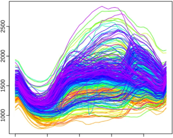
The data set consists of half-hourly electricity demand in South Australia from 6/7/1997 to 31/3/2007. These data were obtained from Australian Energy Market Operator (http: //www.aemo.com.au/). As a vehicle of illustration, we consider the half-hourly electricity demand on Mondays (In the data analyses, we consider the half hourly electricity demand from Mondays to Sundays). A univariate time series display of electricity demand on Mondays from 7/7/1997 to 26/3/2007 is presented in Figure1a, with the same data shown in Figure1bas a time series of curves.
1998 2000 2002 2004 2006 1000 1500 2000 2500 Year Demand (Mega w atts)
(a)A univariate time series display of electricity demand
on Mondays. There are 24384 discrete time points. Each time point represents one dimension.
0 5 10 15 20 1000 1500 2000 2500 Half−hour Demand (Mega w atts)
(b)A functional time series display of electricity demand
on Mondays. There are 508 curves. Each curve has 48 dimensions.
Figure 1:Exploratory plots suggesting that both regular pattern and extreme electricity demand are presented in the Monday electricity demand data between 7/7/1997 and 26/3/2007.
In Figure1b, there are some weeks showing extreme electricity demand and are suspected to be outliers. Because the presence of outliers can seriously affect the performance of modeling and forecasting, we applied the outlier detection method ofHyndman & Shang(2010b). This outlier detection method applies functional principal component analysis to reduce the dimensionality of original curves down to two, and it detects an outlier if it is far from the center of bivariate (first two) principal component scores. As a surrogate of original curves, the bivariate principal component scores can be easily plotted via bivariate bagplot ofRousseeuw et al.(1999), from
which outliers and inliers are separated. The detected outliers correspond to the following dates (15/11/1998, 14/1/2001, 18/2/2001, 19/1/2003, 15/2/2004, 28/11/2004, 22/1/2006, 5/3/2006, 10/12/2006, 4/2/2007, and 18/2/2007). These outliers reflect the extremely high electricity demand during the summer season from December to February and holiday period in South Australia. Consequently, they have been removed from further analyses.
3
Forecasting method
3.1 Functional principal component analysis (FPCA)
The forecasting method utilizes FPCA, which plays an important role in the development of functional data analysis. An account of the statistical properties of FPCA, along with applications of the methodology, are given byFerraty & Vieu(2006) andRamsay & Silverman
(2002,2005). Papers covering the development of FPCA include those ofHyndman & Shang
(2009),Hyndman & Ullah(2007),Reiss & Ogden(2007),Rice & Silverman(1991),Shen(2009) andSilverman(1995,1996). Significant treatments of the theory of FPCA are given byCai & Hall(2006),Dauxois et al.(1982),Delaigle et al.(2009),Hall et al.(2006),Hall & Horowitz
(2007) andHall & Hosseini-Nasab(2006,2009).
When all trajectories are complete, the forecasting method begins by subtracting the time-varying functional mean from the original functional data. The time-time-varying functional mean
µ(x) is estimated by ˆ µ(x) =1 n n X t=1 yt(x),
where{y1(x), . . . , yn(x)}is a time series of curves, which can be obtained using a linear
interpola-tion method. If one seeks a robust estimator, then theL1median of data should be used, and is
denoted by ˆ µ(x) = argmin θ(x) n X t=1 kyt(x)−θt(x)k, wherekg(u)k=Rg2(u)du 1 2
. The algorithm ofH¨ossjer & Croux(1995) can be used to compute ˆ
Using FPCA,{y
1(x)−µˆ(x), . . . , yn(x)−µˆ(x)}can be approximated by the sum of orthogonal
func-tional principal components and their associated principal component scores:
yt(x) = ˆµ(x) + K X
k=1
φk(x) ˆβk,t+et(x), (1)
where{φ1(x),· · ·, φK(x)}represents a set of functional principal components,{βˆ1,t, . . . ,βˆK,t}
rep-resents a set of estimated principal component scores,et(x) is the zero-mean residual function,
andK < nis the number of functional principal components. The optimal value ofK in a given
data set can be determined using a holdout method (see Section4.5for detail).
3.2 Point forecasts
Because the principal component scores are uncorrelated to each other, it is appropriate to forecast each series{βˆk,1, . . . ,βˆk,n;k= 1, . . . , K}using univariate time series models, such as the
ARIMA models (Box et al. 2008). It is noteworthy that the lagged cross correlations are not necessarily zero, but they are likely to be small because the contemporaneous correlations are zero (Hyndman & Ullah 2007,Shen & Huang 2008).
Conditioning on the historical curvesI and the fixed functional principal componentsΦ=
{φ1(x), . . . , φK(x)}, the forecasted curves are expressed as
ˆ ynTS+h|n(x) = E[yn+h(x)|I,Φ] = ˆµ(x) + K X k=1 φk(x) ˆβk,n+h|n, (2)
where ˆβk,n+h|ndenotes anh-step-ahead forecast ofβk,n+h.
4
Updating point forecasts
When the functional time series are segments of a seasonal univariate time series, the most recent trajectory is observed sequentially. When we have observed the first m0time periods
ofyn+1(x), denoted byyn+1(xe) = [yn+1(x1), . . . , yn+1(xm0)] 0
, we are interested in forecasting the data in the remainder of weekn+ 1, denoted byyn+1(xl). However, the TS method described in
the most recent curve. Instead, using (2), the time series forecast ofyn+1(xl) is given by ˆ ynTS+1|n(xl) = E[yn+1(xl)|Il,Φl] = ˆµ(xl) + K X k=1 φk(xl) ˆβk,nTS+1|n, for m0< l≤p,
where Il denotes the historical curves corresponding to the remaining time periods; Φl =
{φ1(xl), . . . , φK(xl)}is a set of the functional principal components corresponding to the
remain-ing time periods; ˆµ(xl) is the time-varying mean function corresponding to the remaining time
periods.
In order to improve point forecast accuracy, it is desirable to update the point forecasts for the rest of weekn+ 1 by incorporating the partially observed data. To address this issue, we review briefly four updating methods recently proposed byShang & Hyndman(2010), and apply them to the electricity demand data.
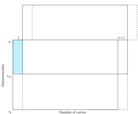
4.1 Block moving (BM) method
The BM method simply redefines the start and end points of our “week” (the time for a single trajectory). Because time is a continuous variable, we can change the support of our trajectories from [1, p] to [m0+ 1, p]∪[1, m0]. xp x1 Dimensionality xm0 n+ 1 Number of curves 1
Figure 2:Update via the block moving approach. The colored region shows the data loss in the first week. The forecasts for the rest of weekn+ 1can be updated by the forecasts using the TS method applied to the top block.
The redefined data are shown diagrammatically in Figure2, where the bottom box has moved to become the top box. The colored region shows the data loss in the first week. The loss of data in the first week will have minimal effect on the forecasts, if the number of curves is large. The partially observed last trajectory under the old function support range completes the last trajectory under the new function support range. The forecasts can be obtained by applying the TS method to the new complete data block.
4.2 Ordinary least squares (OLS) method
We can model and forecast the remaining part of the last trajectory using a regression, based on the functional principal components obtained in (1). LetFebem0∗K matrix whose (j, k)th
entry is φk(xj) for 1≤ j ≤ m0 and 1 ≤k ≤ K. Letβn+1 = [β1,n+1, . . . , βK,n+1]
0
, and n+1(xe) =
[n+1(x1), . . . , n+1(xm0)]0. As the mean-adjusted ˆyn∗+1(xe) =yn+1(xe)−µˆ(xe) becomes available, we
have a regression equation expressed as
ˆ
yn∗+1(xe) =Feβn+1+n+1(xe).
Theβn+1can be estimated via ordinary least squares giving
ˆ
βOLSn+1 = (Fe0Fe)−1Fe0yˆ∗
n+1(xe).
The OLS forecast ofyn+1(xl) is then given by
ˆ ynOLS+1(xl) = E[yn+1(xl)|Il,Φl] = ˆµ(xl) + K X k=1 φk(xl) ˆβOLSk,n+1.
4.3 Ridge regression (RR) method
The OLS method uses the partially observed data in the most recent curve to improve point forecast accuracy for the remaining time periods of week n+ 1, but it needs a sufficiently large number of observations (at least equal toK) in order for ˆβnOLS+1 = [ ˆβ1OLS,n+1, . . . ,βˆK,nOLS+1]0to be numerically stable. To address this problem, we adapt the ridge regression (RR) method ofHoerl & Kennard(1970) with the predictors being the corresponding functional principal components and the partially observed data being the responses. The advantage of RR method is that it uses
a square penalty function, which is rotationally invariant hypersphere centered at the origin (Izenman 2008). Thus, the regression coefficient estimates of the RR method have a closed form. The TS method shrinks the regression coefficient estimates toward zero. The RR coefficient estimates are obtained by minimizing a penalized residual sum of squares
argmin βn+1 n [ ˆyn∗+1(xe)−Feβn+1] 0 [ ˆyn∗+1(xe)−Feβn+1] +λβ 0 n+1βn+1 o , (3)
whereλ >0 is a tuning parameter that controls the amount of shrinkage. By taking the first derivative with respect toβn+1in (3), we obtain
ˆ
βnRR+1=Fe0Fe+λIK−1Fe0yˆ∗
n+1(xe),
whereIK is theK∗K identity matrix. When the penalty parameterλ→0, ˆβnRR+1approaches
ˆ
βnOLS+1, provided thatFe0Fe−1exists; whenλ→ ∞, ˆβRR
n+1approaches 0; when 0< λ <∞, ˆβnRR+1is
a weighted average between 0 and ˆβnOLS+1. The RR forecast ofyn+1(xl) is given by
ˆ ynRR+1(xl) = E[yn+1(xl)|Il,Φl] = ˆµ(xl) + K X k=1 φk(xl) ˆβk,nRR+1.
4.4 Penalized least squares (PLS) method
Although the RR method solves the potential singularity problem of the OLS method, it does not take account of the TS forecasted regression coefficient estimates, ˆβnTS+1|n. This motivates
the development of the PLS method (Shen 2009,Shen & Huang 2008), in which the regression coefficient estimates are selected by shrinking them toward ˆβnTS+1|n. The PLS regression coefficient
estimates minimize a penalized residual sum of squares
arg min βn+1 [ ˆyn∗+1(xe)−Feβˆn+1] 0 [ ˆyn∗+1(xe)−Feβˆn+1] +λ( ˆβn+1−βˆTSn+1|n) 0 ( ˆβn+1−βˆTSn+1|n) . (4)
The first term in (4) measures the “goodness of fit”, while the second term penalized the departure of the regression coefficient estimates from the TS forecasted regression coefficient estimates. The ˆβnPLS+1obtained can thus be seen as a tradeoffbetween these two terms, subject to
a penalty parameterλ. By taking the first derivative with respect to ˆβn+1in (4), we obtain ˆ βnPLS+1= (Fe0Fe+λIK)−1[Fe0yˆ∗ n+1(xe) +λβˆTSn+1|n] = Fe 0 ˆ yn∗+1(xe) Fe0Fe+λIK + λβˆnTS+1|n Fe0Fe+λIK = Fe 0 Fe Fe0Fe+λIK ˆ βnOLS+1+ λ Fe0Fe+λIK ˆ βnTS+1|n = IK− λIK Fe0Fe+λIK ˆ βnOLS+1 + λIK Fe0Fe+λIK ˆ βnTS+1|n.
When the penalty parameterλ→0, ˆβPLS
n+1approaches ˆβnOLS+1, provided that (Fe
0
Fe)−1exists; when
λ→ ∞, ˆβPLS
n+1 approaches ˆβnTS+1|n; when 0< λ <∞, ˆβ
PLS
n+1is a weighted average between ˆβOLSn+1 and
ˆ
βnTS+1|n.
The PLS forecast ofyn+1(xl) is given by
ˆ ynPLS+1(xl) = E[yn+1(xl)|Il,Φl] = ˆµ(xl) + K X k=1 φk(xl) ˆβk,nPLS+1. (5)
4.5 Selections of penalty parameter and number of components
We split the data into a training sample and a testing sample (including one-year electricity demand fromn−51 ton weeks, wheren denotes the total number of weeks, excluding the
outliers). Within the training sample, we further split the data into a training set and a validation set (including electricity demand fromn−103 ton−52 weeks, excluding the outliers).
For a set of possible number of principal componentsK= 1,2, . . . ,10, we apply the TS method to the training set and obtain forecasts for the data in the validation set. The optimal number of component is determined by minimizing the mean absolute percentage error (MAPE) criterion within the validation set. In the Monday electricity demand data, the optimal number of components isK= 3.
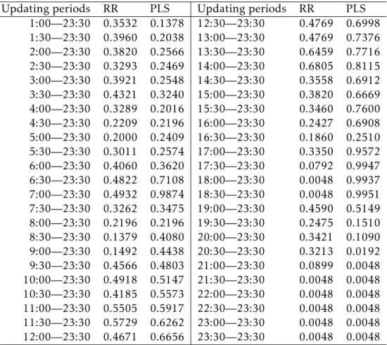
The optimal values of penalty parameterλfor different updating periods are also determined by minimizing the MAPE criterion within the validation set. The MAPE criterion is the most widely used error measure in electricity demand forecasting. It can be expressed as
MAPE = 1 pq q X j=1 p X i=1 ym−j+1(xi)−yˆm−j+1|m−j(xi) ym−j+1(xi) ∗100,
whereprepresents the number of observations in each week,qrepresents the number of weeks in the validation set, andmdenotes the index corresponding to the maximum number of weeks in the validation set (i.e., m=n−52 in the above forecast setting). In Table 1, the optimal
tuning parameters for different updating periods on Mondays are given for both the RR and PLS methods (Due to limited space and repetition, the optimal tuning parameters for different updating periods from Tuesdays to Sundays are availble upon request from the author).
Updating periods RR PLS Updating periods RR PLS
1:00—23:30 0.3532 0.1378 12:30—23:30 0.4769 0.6998 1:30—23:30 0.3960 0.2038 13:00—23:30 0.4769 0.7376 2:00—23:30 0.3820 0.2566 13:30—23:30 0.6459 0.7716 2:30—23:30 0.3293 0.2469 14:00—23:30 0.6805 0.8115 3:00—23:30 0.3921 0.2548 14:30—23:30 0.3558 0.6912 3:30—23:30 0.4321 0.3240 15:00—23:30 0.3820 0.6669 4:00—23:30 0.3289 0.2016 15:30—23:30 0.3460 0.7600 4:30—23:30 0.2209 0.2196 16:00—23:30 0.2427 0.6908 5:00—23:30 0.2000 0.2409 16:30—23:30 0.1860 0.2510 5:30—23:30 0.3011 0.2574 17:00—23:30 0.3350 0.9572 6:00—23:30 0.4060 0.3620 17:30—23:30 0.0792 0.9947 6:30—23:30 0.4822 0.7108 18:00—23:30 0.0048 0.9937 7:00—23:30 0.4932 0.9874 18:30—23:30 0.0048 0.9951 7:30—23:30 0.3262 0.3475 19:00—23:30 0.4590 0.5149 8:00—23:30 0.2196 0.2196 19:30—23:30 0.2475 0.1510 8:30—23:30 0.1379 0.4080 20:00—23:30 0.3421 0.1090 9:00—23:30 0.1492 0.4438 20:30—23:30 0.3213 0.0192 9:30—23:30 0.4566 0.4803 21:00—23:30 0.0899 0.0048 10:00—23:30 0.4918 0.5147 21:30—23:30 0.0048 0.0048 10:30—23:30 0.4185 0.5573 22:00—23:30 0.0048 0.0048 11:00—23:30 0.5505 0.5917 22:30—23:30 0.0048 0.0048 11:30—23:30 0.5729 0.6262 23:00—23:30 0.0048 0.0048 12:00—23:30 0.4671 0.6656 23:30—23:30 0.0048 0.0048
Table 1:For different updating periods, the optimal tuning parameters used in the RR and PLS methods are determined by minimizing the MAPE criterion within the validation set on Mondays.
5
Interval forecast methods
Prediction intervals are a valuable tool for assessing the probabilistic uncertainty associated with point forecasts. As emphasized inChatfield(1993,2000), it is important to provide interval forecasts as well as point forecasts so as to
2. enable different strategies to be planned for a range of possible outcomes indicated by the interval forecasts;
3. compare forecasts from different methods more thoroughly; and 4. explore different scenarios based on different assumptions.
In our forecasting method, there are two sources of errors that need to be taken into account: errors in estimating the regression coefficient estimates and errors in the model residual. In Sections 5.1 and 5.2, we describe a parametric method and a nonparametric method to construct prediction intervals for the TS and BM methods. In Section 5.3, we revisit a nonparametric bootstrap method to update prediction intervals, by incorporating newly observed data in the most recent curve.
5.1 Parametric method to construct prediction intervals
Based on orthogonality and linear additivity, the total forecast variance for the TS method can be approximated by the sum of individual variances (Hyndman & Ullah 2007):
ˆ ϑn+h|n(x) = Var [yn+h(x)|I,Φ]≈ K X k=1 φ2k(x) ˆζk,n+h|n+ ˆvn+h(x),
where ˆζk,n+h|n= Var( ˆβk,n+h|βˆ1, . . . ,βˆn) can be obtained by a time series model, and the model
residual variance ˆvn+h(x) is estimated by averaging model residual square in weekn+h, ˆ2n+h(x),
for eachxvariable. Under the normality assumption, the 100(1−α)% prediction intervals of
yn+h(x) are constructed as follows,
ˆ yn+h|n(x)−zα q ˆ ϑn+h|n(x), yˆn+h|n(x) +zα q ˆ ϑn+h|n(x) ! ,
wherezαis the (1−α/2) standard normal quantile. This will also work for the BM method with
appropriately defined function support range.
5.2 Nonparametric method to construct prediction intervals
We review a nonparametric method used inHyndman & Shang(2009) andShang & Hyndman
(2010) to construct prediction intervals for the TS and BM methods. We can obtain one-step-ahead forecasts for the principal component scores{βk,1, . . . , βk,n;k= 1, . . . , K}, using a univariate
time series model. Let theh-step-ahead forecast errors be given by ˆπk,j= ˆβk,n−j+1|n−j−βˆk,n−j+1,
βk,n+h:
ˆ
βk,nb +h|n= ˆβk,n+h|n+ ˆπk,b∗, for b= 1, . . . , B,
where ˆπbk,∗denotes the bootstrap samples, andBis the number of bootstrap replications.
Assuming the firstK functional principal components approximate the data relatively well, the model residual should contribute nothing but independent and identically distributed random noise. Consequently, we can bootstrap the model residual ˆξnb+h|n(x) by sampling with
replacement from the residual term{ξˆ1(x), . . . ,ξˆn(x)}.
Adding all possible components of variability and assuming that those components of variability do not correlate to each other, we obtainBforecast variants ofyn+h|n(x),
ˆ ynb+h|n(x) = ˆµ(x) + K X k=1 φk(x) ˆβk,nb +h|n+ ˆξ b n+h|n(x).
Hence, the 100(1−α)% prediction intervals are defined as:
ˆ yb, α 2 n+h|n(x), yˆ b,1−α 2 n+h|n(x) .
This will also work for the BM method with appropriately defined function support range.
5.3 Updating interval forecasts
The prediction intervals can also be updated using a nonparametric bootstrap method. First, we bootstrapBsamples of the TS forecasted regression coefficient estimates, ˆβnb,+1TS|n, and these
boot-strapped samples in turn lead to ˆβnb,+1PLS, according to (5). From ˆβnb,+1PLS, we obtainBreplications of ˆ ynb,+1PLS(xl) = ˆµ(xl) + K X k=1 φk(xl) ˆβb,k,nPLS+1+ ˆξnb+1(xl).
Hence, the 100(1−α)% prediction intervals for the updated forecasts are defined asα/2 and
(1−α/2) empirical quantiles of ˆyb,PLS
n+1 (xl). 5.4 Evaluating interval forecasts
According toBaillie & Bollerslev(1992),McNees & Fine(1996) andChristoffersen(1998), the standard evaluation of interval forecasts proceeds by simply comparing the nominal coverage probability to the empirical (conditional) coverage probability. The evaluation of empirical
coverage probability was preformed as follows: for each curve in the testing sample, prediction intervals of one-step-ahead forecasts were computed parametrically and nonparametrically at the 95% nominal coverage probability, and were tested to check if the holdout data points fall within the specific prediction intervals. The empirical coverage probability was calculated as the ratio between the number of observations that fall in the calculated prediction intervals and the total number of observations in the testing sample. Furthermore, we calculated the coverage probability deviance, which is the difference between the empirical and nominal coverage probabilities as a performance measure. Subject to the same average width of prediction intervals, the smaller the coverage probability deviance is, the better the method is.
The average width of prediction intervals is a way to assess which approach gives narrower prediction intervals. It can be expressed as
W = 1 pq q X j=1 p X i=1 yˆ b,1−α/2 n−j+1|n−j(xi)−yˆ b,α/2 n−j+1|n−j(xi) .
The narrower the average width of prediction intervals is, the more informative the method is, subject to the empirical coverage probability being close to the nominal coverage probability.
5.5 Density forecasts
As a by-product of the nonparametric bootstrap method, we can produce kernel density plots for visualizing density forecasts using the bootstrapped forecast variants. This graphical display is useful for visualizing the extremes and the median quantile. As with the kernel density estimate, we select the bandwidth using a pilot estimation of derivatives proposed bySheather & Jones(1991). This bandwidth selection method is based on choosing the bandwidth that minimizes estimates of the mean integrated squared error, which seems to be close to optimal and generally preferred (Venables & Ripley 2002).
6
Results
6.1 Point forecasts
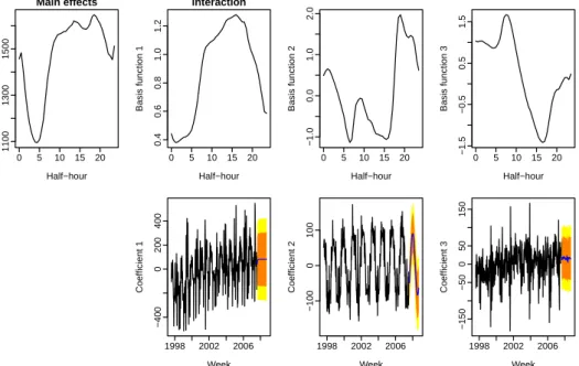
The forecasting method decomposes a functional time series into a number of functional principal components and their associated principal component scores. In the top panel of Figure3, we display and attempt to interpret the first three functional principal components.
Clearly, the mean function illustrates a strong seasonal pattern, with a peak at 18:00 and a trough at 5:00. The functional principal components are of second order effects, as indicated by much smaller scales. The first functional principal component models electricity demand in the afternoon and evening. While the second functional principal component models the contrast in electricity demand between morning and evening, the third functional principal component models the contrast in electricity demand between morning and afternoon.
0 5 10 15 20 1100 1300 1500 Main effects Half−hour Mean 0 5 10 15 20 0.4 0.6 0.8 1.0 1.2 Interaction Half−hour Basis function 1 0 5 10 15 20 −1.0 0.0 1.0 2.0 Half−hour Basis function 2 0 5 10 15 20 −1.5 −0.5 0.5 1.5 Half−hour Basis function 3 Week Coefficient 1 1998 2002 2006 −400 0 200 400 Week Coefficient 2 1998 2002 2006 −100 0 100 Week Coefficient 3 1998 2002 2006 −150 −50 0 50 150
Figure 3:The mean function, the first three functional principal components and their associated principal component scores for the Monday electricity demand from 7/7/1997 to 26/3/2007 (excluding the outliers). The 80% and 95% prediction intervals of the principal component scores are shown by the orange and yellow regions.
The automatic ARIMA algorithm ofHyndman & Khandakar(2008) is a stepwise approach to select the optimal ARIMA model by minimizing Akaike Information Criterion and Bayesian Information Criterion. Using the automatic ARIMA algorithm, we obtained the optimal ARIMA model, from which the principal component scores are forecasted and their 80% and 95% prediction intervals are highlighted by the orange and yellow regions in the bottom panel of Figure3.
By conditioning on the historical data and fixed functional principal components, the fore-casts are obtained by multiplying the forecasted principal component scores with the fixed functional principal components. As an example, Figure 4displays the forecasted Monday electricity demand in the last week of data (i.e., 26/3/2007), along with the 95% parametric and
nonparametric prediction intervals. In this example, we found that the width of the parametric prediction intervals seems to be narrower than the nonparametric counterpart.
0 5 10 15 20 1000 1200 1400 1600 1800 2000 2200 2400 Half−hour Demand (Mega w atts) Forecasts
Parameteric prediction intervals Nonparametric prediciton intervals
Figure 4:Point forecasts of the Monday electricity demand in 26/3/2007, and the 95% prediction intervals constructed via the parametric and nonparametric approaches.
6.2 Point forecast comparisons with some existing methods
By means of comparisons, we also investigate the point forecast accuracy of seasonal autoregres-sive moving average (SARIMA), random walk (RW), and mean predictor (MP) methods. The MP method consists in predicting values at weekt+ 1 by the empirical mean value for each time variable from the first week to thetthweek. The RW approach predicts new values at weekt+ 1 by the observations at weekt. In the forecasting literature, SARIMA has been considered as a benchmark method for forecasting a seasonal time series (Besse et al. 2000,Ferraty et al. 2005). However, it requires the specification of the orders of seasonal components and non-seasonal components. The automatic ARIMA algorithm developed byHyndman & Khandakar(2008) can be used to select the optimal orders for both seasonal and non-seasonal components. To compare their point forecast accuracy, Table2shows the averaged MAPE of the 52 iterative one-step-ahead point forecasts for different updating periods in the testing sample. Using the data in the training set, we forecast the electricity demand for half-hour ahead and calculate the MAPE. By incorporating new observations into the training set, we successively forecast the electricity demand for half-hour ahead. The method that produces the minimal averaged MAPE across all time periods is considered to be the best one. As a result, the four updating methods
Non-dynamic updating methods Dynamic updating methods Updating periods MP RW SARIMA TS BM OLS RR PLS 1:00—23:30 9.9393 7.5067 6.4567 6.6380 6.3717 6.4030 6.4498 6.4658 1:30—23:30 10.0241 7.5869 6.5207 6.7136 6.3909 6.9219 6.8729 6.9087 2:00—23:30 10.1066 7.6658 6.5847 6.7903 6.4640 6.9013 6.9707 6.9871 2:30—23:30 10.1839 7.7447 6.6491 6.8665 6.5687 6.9425 6.8954 6.9066 3:00—23:30 10.2537 7.8235 6.7154 6.9415 6.6080 6.8430 6.8598 6.8891 3:30—23:30 10.3160 7.9072 6.7859 7.0169 6.6259 6.6180 6.5749 6.5989 4:00—23:30 10.3677 7.9955 6.8613 7.0926 6.7594 6.3496 6.3262 6.3400 4:30—23:30 10.4107 8.0871 6.9386 7.1681 6.8499 6.2161 6.2057 6.2122 5:00—23:30 10.4450 8.1816 7.0147 7.2402 6.9559 6.1238 6.1195 6.1226 5:30—23:30 10.4733 8.2761 7.0877 7.3086 7.0207 6.1269 6.1245 6.1265 6:00—23:30 10.4930 8.3617 7.1508 7.3662 7.1019 6.4182 6.7110 6.7301 6:30—23:30 10.5023 8.4420 7.2078 7.4126 7.1010 6.7486 6.7276 6.7384 7:00—23:30 10.4948 8.5095 7.2518 7.4442 7.1837 6.5580 6.5502 6.5561 7:30—23:30 10.4762 8.5693 7.2903 7.4666 7.2146 6.4237 6.4170 6.4201 8:00—23:30 10.4602 8.6223 7.3232 7.4958 7.1763 6.2799 6.2768 6.2784 8:30—23:30 10.4410 8.6686 7.3532 7.5267 7.2338 6.2303 6.2288 6.2298 9:00—23:30 10.4246 8.7111 7.3852 7.5592 7.2023 6.2327 6.2320 6.2326 9:30—23:30 10.4118 8.7559 7.4173 7.5946 7.2633 6.2085 6.2038 6.2069 10:00—23:30 10.3977 8.7951 7.4463 7.6252 7.3626 5.9750 5.9230 5.9370 10:30—23:30 10.3835 8.8267 7.4749 7.6492 7.4509 5.7481 5.7364 5.7458 11:00—23:30 10.3714 8.8509 7.5039 7.6654 7.2585 5.6179 5.6104 5.6177 11:30—23:30 10.3626 8.8691 7.5340 7.6743 7.0264 5.5516 5.5436 5.5506 12:00—23:30 10.3513 8.8818 7.5642 7.6806 6.8234 5.6612 5.6566 5.6613 12:30—23:30 10.3443 8.8844 7.5898 7.6805 6.7780 5.7994 5.7966 5.7999 13:00—23:30 10.3476 8.8761 7.6025 7.6655 6.7226 5.9145 5.9126 5.9151 13:30—23:30 10.3529 8.8479 7.6029 7.6337 6.7328 6.0473 6.0460 6.0479 14:00—23:30 10.3515 8.8088 7.5925 7.5919 6.5597 6.2160 6.2151 6.2165 14:30—23:30 10.3562 8.7542 7.5666 7.5324 6.3209 6.3974 6.3966 6.3978 15:00—23:30 10.3648 8.6846 7.5324 7.4562 6.0053 6.5974 6.5968 6.5977 15:30—23:30 10.3733 8.5930 7.4697 7.3573 5.7507 6.7292 6.7256 6.7266 16:00—23:30 10.3760 8.4770 7.3791 7.2308 5.5620 6.4529 6.4245 6.4253 16:30—23:30 10.3695 8.3352 7.2659 7.0752 5.4975 6.0517 6.0449 6.0444 17:00—23:30 10.3544 8.1706 7.1358 6.8912 5.4994 6.2606 6.2581 6.2576 17:30—23:30 10.3336 7.9876 7.0047 6.6822 5.5173 6.5472 6.5467 6.5463 18:00—23:30 10.2881 7.7883 6.8294 6.4493 5.6643 6.9187 6.9190 6.9186 18:30—23:30 10.1663 7.5652 6.6136 6.2043 5.6307 7.3121 7.3122 7.3121 19:00—23:30 9.9810 7.3339 6.4094 6.0053 5.4354 7.3216 7.3216 7.3217 19:30—23:30 9.7757 7.1090 6.2104 5.8395 5.2703 2.9426 2.9366 2.9356 20:00—23:30 9.5759 6.8838 6.0193 5.6792 5.0626 2.5905 2.5884 2.5882 20:30—23:30 9.3964 6.6490 5.8275 5.5161 4.8095 2.2986 2.2983 2.2979 21:00—23:30 9.2094 6.3991 5.6116 5.3385 4.5848 2.0978 2.0979 2.0976 21:30—23:30 8.9951 6.1284 5.3667 5.1449 4.4028 2.0618 2.0620 2.0618 22:00—23:30 8.7333 5.8180 5.0849 4.9302 4.1887 2.1685 2.1689 2.1687 22:30—23:30 8.4264 5.4437 4.7318 4.6839 4.0672 2.4173 2.4178 2.4176 23:00—23:30 8.2795 5.0244 4.3459 4.4646 3.8888 2.6172 2.6179 2.6175 23:30—23:30 8.9836 4.4998 3.9002 4.2196 4.5676 2.0160 2.0166 2.0162 Mean 10.0832 7.8848 6.7872 6.8089 6.1855 5.5843 5.5856 5.5911
Table 2:Averaged MAPE of the 52 iterative one-step-ahead point forecasts from Monday to Sunday using the MP, RW, SARIMA, TS, BM, OLS, RR and PLS methods for different updating periods in the testing sample. The minimal value of the averaged MAPE is marked in bold.
achieved better point forecast accuracy than the non-updating methods in general. Among the updating methods, the OLS, RR and PLS methods performed equally well for forecasting electricity demand.
We further carried out a pairwisettest to examine whether or not the difference of point forecast accuracy among methods is significant. Based on the MAPE across 46 different time periods, the pairwiset-test given in Table3indicates that the MP method differs significantly from all other methods, as is the RW method. The SARIMA method performs similarly with the TS and BM methods, but it differs significantly from other methods. The four updating methods differs significantly from other non-updating methods, but they perform similarly among each other.
MP RW SARIMA TS BM OLS RR
RW 2.2e-14 - - -
-SARIMA <2e-16 0.00039 - - - -
-TS <2e-16 0.00050 1.00000 - - -
-BM <2e-16 5.4e-09 0.17832 0.16129 - -
-OLS <2e-16 1.5e-15 8.6e-05 7.2e-05 0.17832 -
-RR <2e-16 1.5e-15 8.6e-05 7.2e-05 0.17832 1.00000
-PLS <2e-16 1.7e-15 8.6e-05 7.2e-05 0.17832 1.00000 1.00000
Table 3:Based on the MAPE across 46 different time periods, thep-values of pairedttest statistics are calculated to test the difference in point forecast accuracy among methods.
6.3 Updating interval forecasts
Supposing we observe the electricity demand from midnight to 18:30 in 26/3/2007, it is possible to dynamically update the interval forecasts for the remaining time periods using the BM and PLS methods. Based on the historical data on Mondays (excluding the outliers), we obtain the forecasted principal component scores using the automatic ARIMA models. Utilizing the relationship between ˆβnb,+1TS|nand ˆβ
b,PLS
n+1 , the PLS prediction intervals for the updating time
periods can be obtained from (5). As an example, Figure5presents the 95% prediction intervals obtained by the TS, BM and PLS methods for the electricity demand from 19:00 to 23:30. From Figure 5, the PLS prediction intervals are comparably narrower than the prediction intervals of the TS and BM methods. Thus, they provide more informative evaluation of forecast uncertainty, subject to the same coverage probability. To compare the interval forecast accuracy, Table4shows the average coverage probability deviance and the average width of prediction intervals for different updating time periods in the testing sample.
Coverage probability deviance Prediction interval width
Parametric Nonparametric Parametric Nonparametric
Updating periods TS BM TS BM PLS TS BM TS BM PLS 1:00—23:30 0.017 0.016 0.014 0.037 0.047 562 560 647 643 625 1:30—23:30 0.018 0.017 0.016 0.033 0.045 569 567 653 653 633 2:00—23:30 0.018 0.017 0.013 0.028 0.047 576 574 662 662 639 2:30—23:30 0.019 0.018 0.015 0.035 0.049 583 582 667 667 646 3:00—23:30 0.018 0.018 0.016 0.039 0.047 591 589 680 674 648 3:30—23:30 0.018 0.018 0.014 0.036 0.048 599 597 681 683 649 4:00—23:30 0.018 0.017 0.015 0.036 0.052 607 605 697 688 660 4:30—23:30 0.018 0.017 0.014 0.038 0.048 616 614 705 697 670 5:00—23:30 0.018 0.017 0.014 0.041 0.049 625 623 714 707 680 5:30—23:30 0.019 0.018 0.014 0.039 0.048 634 631 722 715 690 6:00—23:30 0.019 0.018 0.016 0.034 0.052 643 640 736 723 693 6:30—23:30 0.019 0.020 0.015 0.035 0.048 651 647 746 736 705 7:00—23:30 0.020 0.020 0.017 0.034 0.048 658 654 755 733 704 7:30—23:30 0.019 0.019 0.014 0.035 0.049 663 659 761 740 713 8:00—23:30 0.020 0.018 0.016 0.038 0.053 669 663 770 743 696 8:30—23:30 0.019 0.019 0.020 0.035 0.049 673 667 771 745 691 9:00—23:30 0.020 0.019 0.017 0.039 0.054 677 672 781 748 676 9:30—23:30 0.020 0.019 0.017 0.043 0.055 681 678 782 758 669 10:00—23:30 0.021 0.020 0.017 0.045 0.050 684 682 791 761 673 10:30—23:30 0.021 0.021 0.016 0.047 0.059 686 683 790 756 661 11:00—23:30 0.021 0.022 0.020 0.036 0.060 688 678 792 738 654 11:30—23:30 0.020 0.020 0.023 0.037 0.060 689 670 795 722 650 12:00—23:30 0.020 0.023 0.019 0.034 0.055 689 660 794 712 646 12:30—23:30 0.019 0.024 0.023 0.042 0.054 688 651 791 703 629 13:00—23:30 0.020 0.023 0.020 0.038 0.055 686 640 793 691 628 13:30—23:30 0.022 0.023 0.022 0.045 0.057 683 626 787 683 618 14:00—23:30 0.024 0.024 0.021 0.050 0.055 679 607 781 683 612 14:30—23:30 0.024 0.031 0.021 0.052 0.057 673 584 770 681 602 15:00—23:30 0.024 0.027 0.017 0.065 0.053 666 556 758 694 593 15:30—23:30 0.024 0.025 0.022 0.054 0.054 658 532 748 709 582 16:00—23:30 0.025 0.029 0.023 0.042 0.050 647 522 732 719 572 16:30—23:30 0.025 0.030 0.022 0.039 0.052 634 523 713 722 535 17:00—23:30 0.025 0.031 0.022 0.038 0.062 620 528 698 725 501 17:30—23:30 0.026 0.031 0.021 0.041 0.054 604 534 679 706 493 18:00—23:30 0.029 0.028 0.025 0.033 0.062 586 535 658 685 428 18:30—23:30 0.029 0.029 0.019 0.037 0.076 567 529 637 661 367 19:00—23:30 0.029 0.024 0.019 0.065 0.039 548 516 609 619 450 19:30—23:30 0.029 0.026 0.024 0.051 0.048 528 493 584 583 367 20:00—23:30 0.029 0.024 0.026 0.042 0.054 509 474 564 546 340 20:30—23:30 0.030 0.021 0.020 0.037 0.121 489 451 540 513 261 21:00—23:30 0.030 0.019 0.023 0.027 0.138 467 426 509 489 208 21:30—23:30 0.031 0.017 0.031 0.025 0.136 443 396 443 479 157 22:00—23:30 0.029 0.020 0.029 0.027 0.159 417 365 417 473 109 22:30—23:30 0.029 0.023 0.029 0.033 0.144 391 338 391 467 110 23:00—23:30 0.029 0.023 0.029 0.037 0.157 363 317 363 452 111 23:30—23:30 0.030 0.059 0.030 0.044 0.120 340 300 340 469 152 Mean 0.023 0.023 0.020 0.039 0.066 600 566 678 664 539
Table 4:Averaged empirical coverage probability deviance and width of the TS, BM and PLS prediction intervals constructed parametrically and nonparametrically for the 52 iterative one-step-ahead forecasts. The minimal mean coverage probability deviance and the minimal width are marked in bold.
19 20 21 22 23 1200 1400 1600 1800 2000 2200 Half−hour Demand (Mega w atts) Observations
Nonparametric prediction intervals of TS Nonparametric prediction intervals of BM Nonparametric prediction intervals of PLS
Figure 5:The 95% prediction intervals of the Monday electricity demand from 19:00 to 23:30 in 26/3/2007. By incorporating the electricity demand from midnight to 18:30, the prediction intervals can be updated using the nonparametric bootstrap method.
The narrowest width of prediction intervals obtained by the PLS method comes at a cost of the worst coverage probability deviance. The coverage probabilities of the TS and BM methods using the parametric approach are similar; but the BM method produces narrower prediction intervals than the TS method, thus it provides more informative evaluation of uncertainty. An advantage of generating bootstrap samples is to provide density forecasts obtained using kernel density estimation. For example, Figure6displays the kernel density plots of Monday electricity demand in 26/3/2007 at different time periods, based onB= 500 replications.
800 1200 1600 0.000 0.003 0.006 Midnight Density 800 1200 1600 0.000 0.003 0.006 2am 800 1200 1600 0.000 0.003 0.006 4am 800 1200 1600 0.000 0.003 0.006 6am 800 1200 1600 0.000 0.003 0.006 8am Density 800 1200 1600 0.000 0.003 0.006 10am 800 1200 1600 0.000 0.003 0.006 Noon 800 1200 1600 0.000 0.003 0.006 2pm 800 1200 1600 0.000 0.003 0.006 4pm Demand(Megawatts) Density 800 1200 1600 0.000 0.003 0.006 6pm Demand(Megawatts) 800 1200 1600 0.000 0.003 0.006 8pm Demand(Megawatts) 800 1200 1600 0.000 0.003 0.006 10pm Demand(Megawatts)
Figure 6:Kernel density plots of the half-hourly Monday electricity demand in 26/3/2007. The bandwidth of kernel density plots is selected using a pilot estimation of derivatives (Sheather
7
Conclusions
This paper uses half-hourly electricity demand data in South Australia as an empirical study of nonparametric modeling and forecasting methods for prediction from half-hour ahead to one year ahead. The nonparametric forecasting and updating approaches treat the historical data as a time series of curves. Using FPCA, the dimensionality of data is effectively reduced, and the main features in the data are represented by a set of functional principal components, which explain more than 95% of the total variation in all seven electricity demand data sets. The problem of forecasting future electricity demand has been overcame by forecastingK= 3 one-dimensional principal component scores. Conditioning on the historical data and fixed functional principal components, the forecasts are obtained by multiplying the forecasted principal component scores with the fixed functional principal components.
When partial data in the most recent curve are observed, the four updating methods can not only improve point forecast accuracy, but they also eliminate the assumption,N =np, made in
Aneiros-P´erez & Vieu(2008),Antoch et al.(2008),Antoniadis & Sapatinas(2003),Besse et al.
(2000), andFerraty & Vieu(2006, Chapter.12). The BM approach rearranges the observations to form a complete data block, on which the TS method can still be applied. The OLS approach considers the partially observed data in the most recent curve as responses, and uses them to regress against the corresponding functional principal components. It however may suffer from the singularity problem when the number of partially observed data points is less than the number of functional principal components. To overcome this problem, the RR method heavily penalizes those regression coefficient estimates that deviate significantly from ˆβTSn+1|n. Based on
the averaged MAPE over the 52 iterative one-step-ahead point forecasts in the testing sample, the OLS, RR and PLS methods perform equally the best among all of the methods investigated. Furthermore, we used a nonparametric method to construct prediction intervals, and compared the empirical coverage probability to the parametric method. Although the coverage probability of the parametric and nonparametric methods for the TS and BM methods do not differ much, the nonparametric method is appropriate to produce kernel density plots and to construct prediction intervals for the updated forecasts. With a similar empirical coverage probability between the BM and TS methods, the prediction interval width obtained by the BM method is narrower, thus the BM method provides more informative evaluation of forecast uncertainty than the TS method without updating. The narrowest width of prediction intervals obtained by the PLS method comes at a cost of the worst coverage probability.
The aforementioned approaches may seem complicated for calculating point forecasts, updating point forecasts, and constructing parametric and nonparametric prediction intervals, but their implementation is straightforward using theftsapackage ofHyndman & Shang(2010a).
Acknowledgement
The author would like to acknowledge the financial support of postgraduate publication award of Monash University. The manuscript is greatly benefitted from the comments by Professors Rob Hyndman and Vijay Nair. Thanks are also due to the High Performance Computing Center for access to the Monash Sun Grid Cluster for the data analyses.
References
Aneiros-P´erez, G. & Vieu, P. (2008), ‘Nonparametric time series prediction: A semi-functional partial linear modeling’,Journal of Multivariate Analysis99(5), 834–857.
Antoch, J., Prchal, L., De Rosa, M. R. & Sarda, P. (2008), Functional linear regression with functional response: Application to prediction of electricity consumption,inS. Dabo-Niang & F. Ferraty, eds, ‘Functional and Operatorial Statistics’, Springer, Heidelberg, pp. 23–29. Antoniadis, A. & Sapatinas, T. (2003), ‘Wavelet methods for continuous-time prediction using
Hilbert-valued autoregressive processes’,Journal of Multivariate Analysis87(1), 133–158. Baillie, R. T. & Bollerslev, T. (1992), ‘Prediction in dynamic models with time-dependent
conditional variances’,Journal of Econometrics51(1-2), 91–113.
Bajay, S. V. (1983), ‘Long-term electricity demand forecasting models: a review of methodologies’, Electric Power Systems Research6(4), 243–257.
Besse, P. C., Cardot, H. & Stephenson, D. B. (2000), ‘Autoregressive forecasting of some func-tional climatic variations’,Scandinavian Journal of Statistics27(4), 673–687.
Bosq, D. (2000),Linear Processes in Function Spaces: Theory and Applications, Springer, Berlin. Bosq, D. & Blanke, D. (2007),Inference and Prediction in Large Dimensions, John Wiley, Chichester,
England.
Box, G. E. P., Jenkins, G. M. & Reinsel, G. C. (2008),Time Series Analysis: Forecasting and Control, 4th edn, John Wiley, Hoboken, New Jersey.
Cai, T. & Hall, P. (2006), ‘Prediction in functional linear regression’, Annals of Statistics 34(5), 2159–2179.
Chatfield, C. (1993), ‘Calculating interval forecasts’,Journal of Business & Economic Statistics 11(2), 121–135.
Chatfield, C. (2000),Time-series forecasting, Chapman & Hall/CRC, Boca Raton, Florida. Christoffersen, P. F. (1998), ‘Evaluating interval forecasts’, International Economic Review
39(4), 841–862.
Cottet, R. & Smith, M. (2003), ‘Bayesian modeling and forecasting of intraday electricity load’, Journal of the American Statistical Association98(464), 839–849.
Dauxois, J., Pousse, A. & Romain, Y. (1982), ‘Asymptotic theory for the principal component analysis of a vector random function: Some applications to statistical inference’,Journal of Multivariate Analysis12(1), 136–154.
Delaigle, A., Hall, P. & Apanasovich, T. V. (2009), ‘Weighted least squares methods for prediction in the functional data linear model’,Electronic Journal of Statistics3, 865–885.
Ferraty, F., Rabhi, A. & Vieu, P. (2005), ‘Conditional quantiles for dependent functional data with application to the climatic El Ni ˜no phenomenon’,Sankhya: The Indian Journal of Statistics 67(2), 378–398.
Ferraty, F. & Vieu, P. (2006), Nonparametric Functional Data Analysis: Theory and Practice, Springer, New York.
Goia, A., May, C. & Fused, G. (2010), ‘Functional clustering and linear regression for peak load forecasting’,International Journal of Forecasting26(4), 700–711.
Hall, P. & Horowitz, J. L. (2007), ‘Methodology and convergence rates for functional linear regression’,Annals of Statistics35(1), 70–91.
Hall, P. & Hosseini-Nasab, M. (2006), ‘On properties of functional principal components analy-sis’,Journal of the Royal Statistical Society: Series B68(1), 109–126.
Hall, P. & Hosseini-Nasab, M. (2009), ‘Theory for high-order bounds in functional princi-pal components analysis’, Mathematical Proceedings of the Cambridge Philosophical Society 146(1), 225–256.
Hall, P., M ¨uller, H.-G. & Wang, J.-L. (2006), ‘Properties of principal component methods for functional and longitudinal data analysis’,Annals of Statistics34(3), 1493–1517.
Harvey, A. C. & Koopman, S. J. (1993), ‘Forecasting hourly electricity demand using time-varying splines’,Journal of the American Statistical Association88(424), 1228–1242.
Hippert, H. S., Pedreira, C. E. & Souza, R. C. (2001), ‘Neural networks for short-term load forecasting: a review and evaluation’,IEEE Transactions on Power Systems16(1), 44–55. Hoerl, A. E. & Kennard, R. W. (1970), ‘Ridge regression: biased estimation for nonorthogonal
problems’,Technometrics12(1), 55–67.
Hyndman, R. J. & Booth, H. (2008), ‘Stochastic population forecasts using functional data models for mortality, fertility and migration’,International Journal of Forecasting24(3), 323–342. Hyndman, R. J. & Fan, S. (2010), ‘Density forecasting for long-term peak electricity demand’,
IEEE Transactions on Power Systems25(2), 1142–1153.
Hyndman, R. J. & Khandakar, Y. (2008), ‘Automatic time series forecasting: the forecast package for R’,Journal of Statistical Software27(3).
Hyndman, R. J. & Shang, H. L. (2009), ‘Forecasting functional time series (with discussion)’, Journal of the Korean Statistical Society38(3), 199–221.
Hyndman, R. J. & Shang, H. L. (2010a),ftsa: Functional time series analysis. R package version 1.6.
URL:http://CRAN.R-project.org/package=ftsa
Hyndman, R. J. & Shang, H. L. (2010b), ‘Rainbow plots, bagplots, and boxplots for functional data’,Journal of Computational and Graphical Statistics19(1), 29–45.
Hyndman, R. J. & Ullah, M. S. (2007), ‘Robust forecasting of mortality and fertility rates: A functional data approach’,Computational Statistics & Data Analysis51(10), 4942–4956. Izenman, A. J. (2008),Modern multivariate statistical techniques: regression, classification, and
manifold learning, Springer, New York.
McNees, S. K. & Fine, L. K. (1996), Forecast uncertainty: can it be measured?,in‘Paper presented at the Conference on Expectations in Economics,’, Federal Reserve Bank of Philadelphia. Pedregal, D. J. & Young, P. C. (2008), ‘Development of improved adaptive approaches to
electricity demand forecasting’,Journal of the Operational Research Society59(8), 1066–1076. Preda, C. & Saporta, G. (2005a), ‘Clusterwise PLS regression on a stochastic process’,
Computa-tional Statistics & Data Analysis49(1), 99–108.
Preda, C. & Saporta, G. (2005b), ‘PLS regression on a stochastic process’,Computational Statistics & Data Analysis48(1), 149–158.
Ramsay, J. O. & Silverman, B. W. (2002),Applied Functional Data Analysis: Methods and Case Studies, Springer, New York.
Reiss, P. T. & Ogden, T. R. (2007), ‘Functional principal component regression and functional partial least squares’,Journal of the American Statistical Association102(479), 984–996. Rice, J. A. & Silverman, B. W. (1991), ‘Estimating the mean and covariance structure
non-parametrically when the data are curves’, Journal of the Royal Statistical Society: Series B 53(1), 233–243.
Rousseeuw, P., Ruts, I. & Tukey, J. (1999), ‘The bagplot: A bivariate boxplot’, The American Statistician53(4), 382–387.
Shang, H. L. & Hyndman, R. J. (2010), ‘Nonparametric time series forecasting with dynamic updating’,Mathematics and Computers in Simulationin press.
Sheather, S. J. & Jones, M. C. (1991), ‘A reliable data-based bandwidth selection method for kernel density estimation’,Journal of the Royal Statistical Society: Series B53(3), 683–690. Shen, H. (2009), ‘On modeling and forecasting time series of smooth curves’, Technometrics
51(3), 227–238.
Shen, H. & Huang, J. Z. (2008), ‘Interday forecasting and intraday updating of call center arrivals’,Manufacturing & Service Operations Management10(3), 391–410.
Silverman, B. W. (1995), ‘Incorporating parametric effects into functional principal components’, Journal of the Royal Statistical Society: Series B57(4), 673–689.
Silverman, B. W. (1996), ‘Smoothed functional principal components analysis by choice of norm’,Annals of Statistics24(1), 1–24.
Taylor, J. W. (2003), ‘Short-term electricity demand forecasting using double seasonal exponen-tial smoothing’,Journal of the Operational Research Society54(8), 799–805.
Taylor, J. W. & McSharry, P. E. (2007), ‘Short-term load forecasting methods: an evaluation based on European data’,IEEE Transactions on Power Systems22(4), 2213–2219.
Venables, W. N. & Ripley, B. D. (2002),Modern applied statistics with S, 4th edn, Springer, New York.
Weron, R. (2006),Modeling and forecasting electricity loads and prices: A statistical approach, Wiley, Chichester.