Modeling Yield Risk Under Technological
Change: Dynamic Yield Distributions
and the U.S. Crop Insurance Program
Ying Zhu, Barry K. Goodwin, and Sujit K. Ghosh
The objective of this study is to evaluate the risk associated with major agricultural commodity yields in the United States. We are particularly concerned with the non-stationary nature of the yield distribution, which arises primarily as a result of techno-logical progress and changing environmental conditions over time. In contrast to common two-stage methods, we propose an alternative parametric model that allows the moments of yield distributions to change with time. Several model selection techniques suggest the proposed time-varying model outperforms more conventional models in terms of in-sample goodness-of-fit, out-of-in-sample predictive power, and the prediction accuracy of insurance premium rates.
Key Words: crop insurance, model comparison, time-varying distribution
Introduction
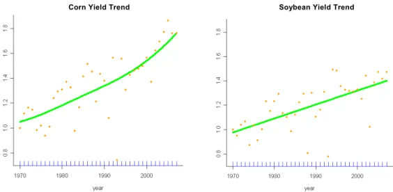
The Federal Crop Insurance program represents an important component of U.S. agricultural policy and is intended to protect farmers from yield and revenue risk. Accurate modeling of crop yield distributions is essential for the proper design of crop insurance contracts and to the maintenance of an actuarially-sound insurance program. Historical agricultural yield data suggest a strong upward trend in crop yields [see figure 1(a)]. Advances in technology, germ- plasm, breeding techniques, the development of new hybrids, and changes in environmental factors may significantly affect the distributions of crop yields. These changes can complicate efforts to accurately model yield distributions using data observed over time.
Many studies have attempted to determine the distributional model and estimation methods that best characterize crop yield distributions. Modeling approaches in the current literature range from nonparametric (Goodwin and Ker, 1998) to parametric methods (Day, 1965; Nelson and Preckel, 1989; Taylor, 1990; Ramirez, 1997; Ramirez, Misra, and Field, 2003; Just and Weninger, 1999; Chen and Miranda, 2004; Sherrick et al., 2004, among others) based on the assumption that crop yields are independently and identically distributed. The parametric approach of modeling yields usually involves selection and specification of candidate distri-bution families, parameter estimation, and goodness-of-fit assessments. Among others, the Beta distribution is popularly used in practice because of its flexibility and ability to represent the skewness typically associated with crop yield distributions. The concept of a conditional Beta distribution for yields was introduced by Nelson and Preckel (1989). Other popular
Ying Zhu is a research statistician, SAS Institute, Inc., and former graduate student, Department of Agricultural and Resource Economics, North Carolina State University; Barry K. Goodwin is the William Neal Reynolds Professor, Department of Agricultural and Resource Economics, North Carolina State University; and Sujit K. Ghosh is a professor, Department of Statistics, North Carolina State University. The helpful comments of three anonymous referees are gratefully acknowledged.
candidates used in the literature include the lognormal distribution (Day, 1965), the normal distribution (Just and Weninger, 1999), the normal distribution with spatial effects (Ozaki et al., 2008). the Weibull distribution (Chen and Miranda, 2004), and the logistic distribution (Sherrick et al., 2004). Evidence of nonnormal yields has been presented by a number of authors, including Taylor (1990), Ramirez (1997), and Ramirez, Misra, and Field (2003). In many cases, agricultural yields display a strong upward trend over time, and the deviations from trend (residuals) frequently display heteroskedasticity [see figure 1(a)], violating the assumption that yields are identically distributed. A common approach to modeling yield risk using time-series data has been to first detrend the time-series data and then estimate the yield distribution using the detrended yield data, treating the estimated, detrended yields as “observed” data. These approaches are often referred to as “two-stage” methods; the first stage fits a trend model to the data, while the second stage uses the detrended data to model the distribution. Examples of such two-stage detrending procedures can be found in Miranda and Glauber (1997), Swinton and King (1991), and Atwood, Shaik, and Watts (2003), among others. In this two-stage method, it is crucial to determine the correct functional form of the regression that represents trend in the first stage and then to establish the correct distributional properties of the detrended data, including such characteristics as skewness, kurtosis, and heteroskedasticity. Yet, it has been recognized that the resulting estimated residuals, represent- ing the detrended yields, are subject to the estimation uncertainty associated with sampling variability in the first-stage estimates of trend, and thus may not necessarily provide an accurate representation of the actual yield distribution. Any biases induced at the first stage asymptotically approach zero when the correct functional form is used in the regression and errors are homoskedastic. However, the uncertainty introduced at the first stage, if not accounted for in second-stage estimates of the yield distribution, will lead to inaccurate esti-mation of variance in the final estimates. The magnitude of this effect can be large especially when the errors are heteroskedastic (Robinson, 1987) and can potentially introduce significant adverse selection into an insurance program if ignored.
This standard two-stage method is among the most popular approaches to removing time trends and modeling the distribution of crop yields. A similar two-stage method is used to rate the Group Risk (GRP) and Gross Revenue Insurance (GRIP) programs, though this method does address the potential for heteroskedasticity. However, it is possible to account for the uncertainties associated with the first-stage estimates and adequately represent characteristics of the yield distribution (such as deterministic trends and heteroskedasticity) by applying an alternative simultaneous estimation method. We propose a likelihood-based estimation method that simultaneously estimates the trend (conditional mean) and higher order conditional moments of the yield density by using a flexible class of parametric distributions. We also pro-vide a set of model validation tools for enabling a researcher to test the validity of the proposed class of distributions in approximating the true underlying data-generation mechanism.
This method, along with the validation measures proposed here, allows one to measure conditional yield risk in a dynamic setting and thereby calculate premium rates for crop insur-ance contracts in a more accurate and systematic way. Our method essentially models the first four conditional moments of the distribution simultaneously by allowing location, scale, skew-ness, and kutosis parameters of the specific distributional family to evolve over time.The more common two-stage method usually allows one to model only the location (conditional mean) and sometimes the scale (conditional variance) to reflect changes over time. A more complete and coherent picture of technological progress and the consequential changes in yield risk can be provided by simultaneously modeling the time trend and the distributional parameters.
Corn Yield Trend Soybean Yield Trend
(a) Yield trend of different crops (1970–2007)
(b) Residual plot of annual corn yield, Adair County, Iowa
A Conventional Two-Stage Estimation Framework
In most empirical analyses, a deterministic trend is used to capture the dynamics of the expected yields, and thus to represent the variation of yields around this expected level.1 The trend component is usually controlled for prior to assessing the distribution of yields— generally using a homoskedastic parametric or nonparametric regression model. Popular regression models include a log-linear specification based on polynomials, kernel regression, smoothing splines, and partial linear models (Gyorfi et al., 2002). We illustrate this idea by using a quadratic trend as well as a nonparametric trend model.2
Consider the following trend model:
(1) ytm x( )t t,
where yt is the observed crop yield in year t, (t =1,..., T); m(x) denotes the regression function E(Yt | Xt = x); xt signifies linear or nonlinear time indexes representing trend; and εt represents residuals that are assumed to be independently distributed with mean zero. The regression function m(·) can be estimated nonparametrically using kernel methods or smoothing spline methods. Alternatively, if we assume a parametric functional form for m(·), then the regression coefficients can be obtained using ordinary least squares (OLS).3 In either case, the residuals are obtained as ˆt ytm xˆ ( ).t We considered both quadratic and
non-parametric trend models. The Kolmogorov-Smirnov (K-S) two-sample goodness-of-fit (GOF) test suggests that the two residual distributions are not significantly different between the nonparametric and parametric models based on the data in this study. On the basis of this test, the quadratic detrending method is used as a benchmark.
The empirical analyses presented in this paper are based on applications to the USDA’s National Agricultural Statistics Service (NASS) county-level average yields.4 Figure 1(b) presents the nonparametric residual plot of annual corn yields in Iowa, which shows that the deviations from trend tend to be proportional to the level of the yields. To account for this temporal heteroskedasticity effect, a rescaled form of the deviations from a trend-based, forecasting equation is often suggested. This approach, though ad hoc, is commonly used in practice (see, e.g., Miranda and Glauber, 1997; Atwood, Shaik, and Watts, 2003). By dividing each error by its associated forecast, the residuals can be scaled to the year T equivalent predicted yield.
We use a goodness-of-fit (GOF) specification test to determine the appropriate distribution for the detrended yield .yt A Q-Q plot based on the residuals t [figure 1(b)] indicates the
residuals are more negatively skewed than what would be implied by the normal distribution, which suggests that a Beta distribution may be a viable candidate. A GOF test for the Beta distribution (based on a χ2 statistic) confirms that a Beta distribution provides a reasonable fit for the normalized county-level yields typically applied in this two-stage approach. For
1The main justification for using a deterministic component is that if crop yield variables evolve slowly through time, then approximation of a deterministic component may be sufficient to model the yield distribution (Just and Weninger, 1999).
2The selection of these two trend models is intended to provide a benchmark for comparison purposes. There are other detrending methods such as log-linear regression. Since the focus of this study is to compare the two-stage approach and the time-varying method proposed here as an alternative, we use representative methods to illustrate the concepts. A comprehensive survey of all possible detrending methods is beyond the scope of this study.
3We assume that m(x
t) = m0(xt, β), where m0 is a known functional form up to some finite dimensional regression coefficient vector β.
example, the GOF test of Iowa all-practice corn yields produces a p-value of 0.51 for Kossuth County and 0.62 for Adair County. We use Beta(α, β, θ, δ) to denote a Beta distribution with shape parameters α, β > 0, location parameter θ≥ 0, and scale parameter δ > 0.5 This implies the yields follow a Beta distribution with constant shape parameters and time-varying location and scale parameters; specifically, yt: Beta(α, β, t, ),t with t ˆt , t ˆt ,and
ˆt y yˆt/ˆT.
The log-likelihood function of a general Beta distribution based on the detrended data yt with two shape parameters α and β, location θ, and scale parameters δ is given by:
(2)
1 1 1 1 ( , , , | , 1, , ) ( 1)log( ) ( 1)log( ) log ( , ) ( 1)log( ) , t T T t t t t T T t t LLF y t T y y B
where log(B(α, β)) = log(Γ(α)) + log(Γ(β)) – log(Γ(α + β)), and log(a+) = log(a) if a > 0
and log(a+) = 0 otherwise, which ensures that ,
t
y t
for any θ, δ > 0.
We obtain the parameter estimates ( , , , ) ˆ ˆ ˆ ˆ by maximizing the LLF(α, β, θ, δ) based on the normalized values of .yt The results are presented in table 1. The predicted mean yield can be calculated from the detrended model as:
(3) ˆˆ ˆ ˆ ˆ ( ) ˆ ˆ ˆ ˆ . ˆ ˆ ( ) ˆ T T t t t t y m x y y y m x
As previously noted, using a first-stage estimation to detrend yield data and then treating the resulting detrended yields as if they were observed without error may not be appropriate because the first-stage estimation error is ignored [i.e.,ˆ st, are assumed to be known for the
LLF in equation (2)]. A more systematic inferential method may be needed to accurately capture trend effects and model conditional yield risk.
A Time-Varying Yield Distribution Model
In this section, a flexible class of parametric models is proposed, which allows us to simul-taneously and coherently specify the first four moments using suitable polynomials of time. The coefficients of the polynomials are estimated simultaneously by maximizing the resulting likelihood function. Several alternative models are examined to measure conditional yield risk. For instance, instead of using polynomials to model the first four moments of the pro-posed distribution, one may use knot-based splines. In contrast to typical methods, the time-varying model accounts for parameter uncertainty by maximizing the time-time-varying likelihood function, which includes time-trend parameters and the distributional parameters in one step. The results of this proposed model are compared to those based on the conventional two-stage approach described in the previous section for several important crops and counties drawn from U.S. county-level data.
5 In other words,( ) / : ( , ), t
y Beta where Beta(α, β) represents a standard Beta distribution defined on (0, 1) with shape parameters α, β > 0.
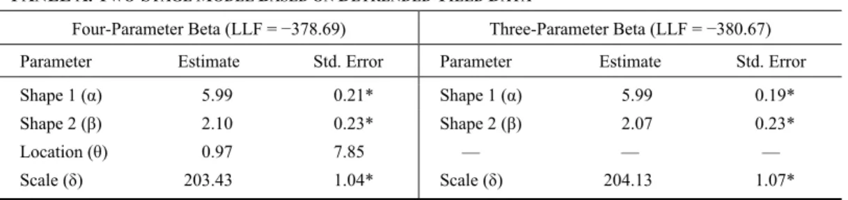
Table 1. Maximum-Likelihood Parameter Estimates and Summary Statistics for Two-Stage Model and Time-Varying Models: Example for Adair County Corn Yields
PANEL A. TWO-STAGE MODEL BASED ON DETRENDED YIELD DATA
Four-Parameter Beta (LLF = −378.69) Three-Parameter Beta (LLF = −380.67) Parameter Estimate Std. Error Parameter Estimate Std. Error
Shape 1 (α) 5.99 0.21* Shape 1 (α) 5.99 0.19* Shape 2 (β) 2.10 0.23* Shape 2 (β) 2.07 0.23* Location (θ) 0.97 7.85 — — —
Scale (δ) 203.43 1.04* Scale (δ) 204.13 1.07*
PANEL B. TIME-VARYING MODELS BASED ON ACTUAL YIELD DATA
Linear Trend Structure a (LLF = −328.68) Quadratic Trend Structureb (LLF = −326.62)
Parameter Estimate Std. Error Parameter Estimate Std. Error
b1 2.38 0.32* b1 2.55 0.10* b2 0.43 0.75 b2 0.16 0.40 b3 — — b3 −0.29 0.50 b4 4.02 0.32* b4 2.95 0.10* b5 −2.71 1.29* b5 −1.63 0.30* b6 — — b6 −2.61 4.80 b7 7.47 14.99 b7 12.26 117.70 b8 −7.50 18.14 b8 −15.27 138.15 b9 — — b9 −13.72 90.03 Time-Varying Models: LLF(L): L1 = −328.68, L2 = −326.62 LRT Statistics: −2(L1 – L2) = 4.12, 2 [4], p-Value = 0.39
Notes: An asterisk (*) denotes statistical significance at the α = 0.05 or smaller level. Examples for other crops and counties are available from the authors upon request.
aThe time-varying beta model with a linear trend structure is defined as: ~ ( , , 0, ),
t t t t
y where t exp(b1b t2), t exp(b4b t5), and t exp(b7b t8).
bThe time-varying beta model with a quadratic trend structure is defined as: ~ ( , , 0, ),
t t t t
y where t exp(b1b t b t2 32), t exp(b4b t5b t62), and t exp(b7b t b t8 92).
The basic assumption of the time-varying model is that the parameters of the distribution follow a specific temporal pattern, whereby temporal changes of the yield distribution can be captured by the time-varying shape and scale parameters. The resulting parameter estimates are consistently estimated if the likelihood function is appropriately specified.
These time varying parameters evolve according to an exponential form. This particular functional form ensures that the Beta shape, scale, and location parameters are positive at every observation. We evaluated two different time trend structures for the parameters of the yield distributions—a standard linear trend and a quadratic trend model. However, our method is not restricted to these chosen functional forms.6 The log-likelihood function of the
6 Of course, other functional forms—including quadratic specifications—could be used to ensure positive parameters. For instance, we can model any of these Beta parameters generally as exp{ J1 ( ) },
j j
j t b
where the ψj(·)’s may represent members of collection of J basis functions [e.g., choosing ( ) j1,
j t t
we obtain polynomials, while choosing ( ) ( ) ,3
j t t tj
we obtain cubic polynomials with knots tj’s]. Alternatively, one may also specify functional form using the first four moments of the Beta distribution, which may require a constrained optimization of the likelihood function.
time-varying Beta distribution is identical to that of the constant Beta distribution [equation (2)] with the notable exception that the shape and scale parameters are allowed to vary with time and thus appear as αt, βt, δt, and θt.
Because the quadratic specification nests the linear trend, a standard likelihood-ratio test can be used to evaluate the statistical significance of the quadratic terms, and thus to select the optimal trend specification. Note that the Beta distribution is characterized by four parameters (α, β, θ, and δ). For simplicity and numerical stability of the maximum-likelihood approach, we fix the minimum possible yield to be equal to zero in each case (i.e., we set θt = 0 for all t). Each parameter of the Beta distribution is allowed to vary over time through a functional relationship of the form (e.g., α = exp(f(b, t)), where f(·) is a linear or quadratic function of time]. This specification allows us to use an unconstrained maximization of the likelihood function. The quadratic terms were not found to be statistically significant for the data sets we have analyzed, and therefore our final representation of the conditional moments uses a standard linear trend.
The predicted value ˆyt from the time-varying model is given by:
(4) ˆ ˆ ˆ ˆ , ˆ t t t t t y where t ( , ),t b t ( , ), andt b t ( , ).t b Empirical Application
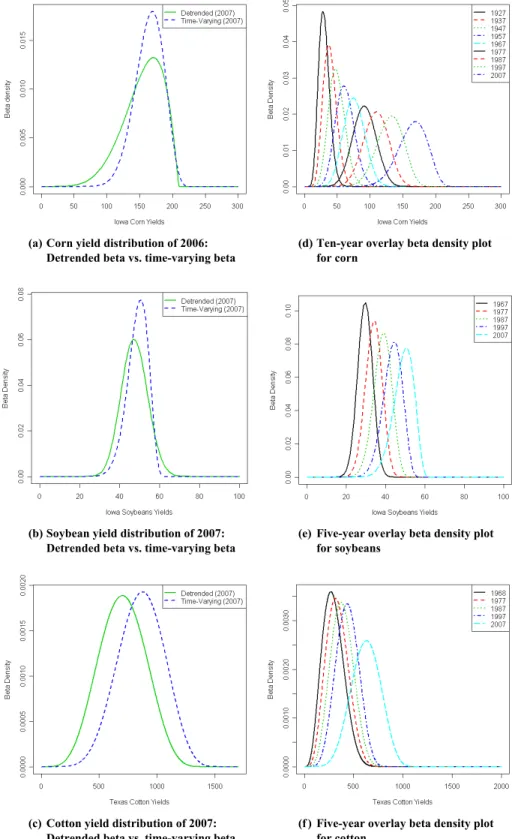
The time-varying model not only addresses the dynamic characteristics of yield distributions, but also provides a more flexible specification of heteroskedasticity and higher order moments (e.g., skewness and kurtosis). We implement the time-varying model by applying the methods to the top 10 counties in the major producing states for corn, soybeans, and cotton. These county/crop combinations include the following: Iowa all-practice corn from Kossuth, Sioux, Pottawattamie, Plymouth, Webster, Pocohontas, Hardin, Franklin, Clinton, and Woodbury counties; Iowa soybeans from Kossuth, Sioux, Pattawattamie, Plymouth, Webster, Woodbury, Benton, Grundy, Crawford, and Tama counties; and Texas upland cotton from Gaines, Lubbock, Hockley, Lynn, Dawson, Hale, Terry, Crosby, Floyd, and Martin counties.7 It is widely recognized that the rate of technological progress varies considerably across different crops. Our results (presented in figure 2) demonstrate that Iowa corn and soybean yields are skewed, kurtotic, and exhibit strong time trend effects and varying degrees of hetero-skedasticity through time. In contrast, Texas cotton yields appear to have a more modest time trend, although strong evidence of temporal heteroskedasticity is exhibited.
Table 1 reports the maximum-likelihood estimates (MLEs) of this time-varying Beta distri-bution with a linear time trend in the exponent and a quadratic time trend structure. A likelihood-ratio test statistic (Wilks, 1938) of the two alternative models has a value of 4.12, which does not reject the null hypothesis that the quadratic trend parameters are equal to zero and thus supports the adequacy of the linear specification.
7 Although our choice of counties encompasses a significant proportion of the overall production of each crop in the relevant states (and further reflects a significant amount of the GRP crop insurance liability and premium), we also considered analysis for a much wider range of all counties (for which data existed) in each state evaluated. The results were very consistent with what is presented below. In order to conserve space, we only present results for the top 10 counties in prominent states for each crop. However, detailed results for other counties are available from the authors on request. In addition, analysis of shorter series of yield data were also considered and found to yield similar conclusions. These results are also available on request.
(a) Corn yield distribution of 2006: Detrended beta vs. time-varying beta
(d) Ten-year overlay beta density plot
for corn
(b) Soybean yield distribution of 2007:
Detrended beta vs. time-varying beta
(e) Five-year overlay beta density plot
for soybeans
(c) Cotton yield distribution of 2007:
Detrended beta vs. time-varying beta
(f ) Five-year overlay beta density plot
for cotton
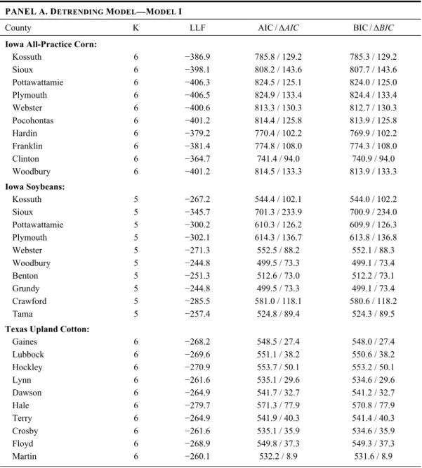
Table 2. Model Comparison Using In-Sample Goodness-of-Fit Test and Nonnested Vuong’s Test for Major Agricultural Yields
PANELA.DETRENDING MODEL—MODEL I
County K LLF AIC /ΔAIC BIC/ΔBIC Iowa All-Practice Corn:
Kossuth 6 −386.9 785.8 / 129.2 785.3 / 129.2 Sioux 6 −398.1 808.2 / 143.6 807.7 / 143.6 Pottawattamie 6 −406.3 824.5 / 125.1 824.0 / 125.0 Plymouth 6 −406.5 824.9 / 133.4 824.4 / 133.4 Webster 6 −400.6 813.3 / 130.3 812.7 / 130.3 Pocohontas 6 −401.2 814.4 / 125.8 813.9 / 125.8 Hardin 6 −379.2 770.4 / 102.2 769.9 / 102.2 Franklin 6 −381.4 774.8 / 108.0 774.3 / 108.0 Clinton 6 −364.7 741.4 / 94.0 740.9 / 94.0 Woodbury 6 −401.2 814.5 / 133.3 813.9 / 133.3 Iowa Soybeans: Kossuth 5 −267.2 544.4 / 102.1 544.0 / 102.2 Sioux 5 −345.7 701.3 / 233.9 700.9 / 234.0 Pottawattamie 5 −300.2 610.3 / 126.2 609.9 / 126.3 Plymouth 5 −302.1 614.3 / 136.7 613.8 / 136.8 Webster 5 −271.3 552.5 / 88.2 552.1 / 88.3 Woodbury 5 −244.8 499.5 / 73.3 499.1 / 73.4 Benton 5 −251.3 512.6 / 73.0 512.2 / 73.1 Grundy 5 −244.8 499.5 / 73.3 499.1 / 73.4 Crawford 5 −285.5 581.0 / 118.1 580.6 / 118.2 Tama 5 −257.4 524.8 / 89.4 524.3 / 89.5
Texas Upland Cotton:
Gaines 6 −268.2 548.5 / 27.4 548.0 / 27.4 Lubbock 6 −269.6 551.1 / 38.2 550.6 / 38.2 Hockley 6 −270.9 553.7 / 50.1 553.2 / 50.1 Lynn 6 −261.6 535.1 / 29.6 534.6 / 29.6 Dawson 6 −264.9 541.7 / 32.7 541.2 / 32.7 Hale 6 −279.7 571.3 / 77.9 570.8 / 77.9 Terry 6 −264.9 541.9 / 40.3 541.4 / 40.3 Crosby 6 −261.6 535.1 / 35.9 534.6 / 35.9 Floyd 6 −268.9 549.8 / 37.3 549.3 / 37.3 Martin 6 −260.1 532.2 / 8.9 531.6 / 8.9
Notes: An asterisk (*) denotes statistical significance at the α = 0.05 or smaller level. K is the number of parameters in a model, LLF is log-likelihood function, and v is Vuong’s test statistic for time-varying model vs. detrending model.
( extended ... → ) The MLEs can be used to evaluate the time-varying Beta density for any given year. Figures 2(d), (e), and (f) illustrate the dynamic evolution of the densities that are estimated by each time-varying model for corn, soybean, and cotton yields, respectively. Various moments of the distributions appear to evolve over time. The density plots of these estimated time-varying distri- butions suggest different means, skewness coefficients, and maximum values of corn yields for each year. Figures 2(a), (b), and (c) present estimated densities for both the time-varying model and the more conventional detrended model. In every case, the time-varying densities show a smaller degree of leptokurtosis than is the case for standard, two-stage detrended yield data.
Table 2. Extended
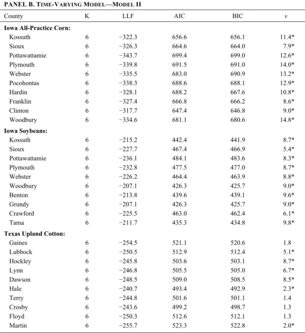
PANELB.TIME-VARYING MODEL—MODEL II
County K LLF AIC BIC v Iowa All-Practice Corn:
Kossuth 6 −322.3 656.6 656.1 11.4* Sioux 6 −326.3 664.6 664.0 7.9* Pottawattamie 6 −343.7 699.4 699.0 12.6* Plymouth 6 −339.8 691.5 691.0 14.0* Webster 6 −335.5 683.0 690.9 13.2* Pocohontas 6 −338.3 688.6 688.1 12.9* Hardin 6 −328.1 688.2 667.6 10.8* Franklin 6 −327.4 666.8 666.2 8.6* Clinton 6 −317.7 647.4 646.8 9.0* Woodbury 6 −334.6 681.1 680.6 14.8* Iowa Soybeans: Kossuth 6 −215.2 442.4 441.9 8.7* Sioux 6 −227.7 467.4 466.9 5.4* Pottawattamie 6 −236.1 484.1 483.6 8.3* Plymouth 6 −232.8 477.5 477.0 8.7* Webster 6 −226.2 464.4 463.9 8.8* Woodbury 6 −207.1 426.3 425.7 9.0* Benton 6 −213.8 439.6 439.1 9.6* Grundy 6 −207.1 426.3 425.7 9.0* Crawford 6 −225.5 463.0 462.4 6.1* Tama 6 −211.7 435.3 434.8 9.8*
Texas Upland Cotton:
Gaines 6 −254.5 521.1 520.6 1.8 Lubbock 6 −250.5 512.9 512.4 5.1* Hockley 6 −245.8 503.6 503.1 8.7* Lynn 6 −246.8 505.5 505.0 6.7* Dawson 6 −248.5 509.0 508.5 8.5* Hale 6 −240.7 493.4 492.9 2.3* Terry 6 −244.8 501.6 501.1 1.4 Crosby 6 −243.6 499.2 498.7 1.3 Floyd 6 −250.3 512.6 512.1 1.3 Martin 6 −255.7 523.3 522.8 2.0*
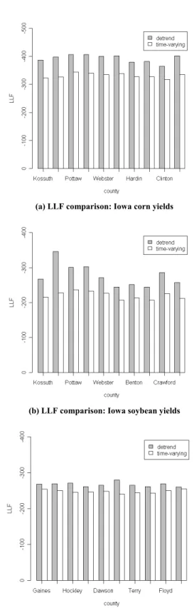
Table 2 reports log-likelihood values for the two alternative models for a number of counties. In almost every case, the time-varying model provides a superior fit to the data when compared to the conventional model, even after adjustments (within the context of alternative information criteria) for the number of parameters. These findings are also illustrated in figure 3, which contains a side-by-side bar plot of the LLF values for all major county/crop combinations considered in our analysis.8
(a) LLF comparison: Iowa corn yields
(b) LLF comparison: Iowa soybean yields
(c) LLF comparison: Texas cotton yields
Figure 3. In-sample goodness-of-fit comparison of the two competing models: Log likelihood function
Model Performance and Specification Tests
We considered a number of specification tests and evaluations of forecasting performance of the alternative models. Vuong’s (1989) nonnested specification test is a likelihood-based test for model selection. Vuong’s test statistic is given by:
(5) 1/2 ( ,ˆ ) , ˆ n n n n n LR v
whereLRn( , ˆn n) Lnf( ) ˆn Lng( );n Lnf( )ˆn is the maximum-likelihood function of the time- varying model;Lng( )n is the maximum-likelihood function of the two-step model; andˆn is defined as: (6) 2 2 2 1 1 ˆ ˆ ( | ; ) ( | ; ) 1 1 ˆ log log . ( | ; ) ( | ; ) n n t t n t t n n t t t n t t t n f Y X f Y X n g Y X n g Y X
The test statistic v is approximately distributed as a standard normal random variable. As specified, if v > c, where c is the critical value,9 we reject the null hypothesis that the models are the same in favor of the alternative time-varying model Fθ. Alternatively, if v ≤−c, we would reject the null in favor of the detrended model Gθ. Vuong’s test statistics (v) are presented in table 2, and in a majority of cases (87%) they support the time-varying specification.
Table 2 also presents goodness-of-fit comparisons for conventional models (model I) and time-varying models (model II) based on the Akaike (1974) information criterion (AIC) and Schwarz’s (1978) Bayesian information criterion (BIC). Smaller values of the AIC or BIC indicate a better fit. Both figure 3 and table 2 show that the time-varying Beta has the lowest AIC and BIC for most or all counties, which confirms it is the most parsimonious and optimal model we have considered. Moreover, ΔAIC(ΔAIC = AIC – min(AIC)) and ΔBIC(ΔBIC = BIC – min(BIC)) in table 2 are significantly large for the conventional detrended Beta model,10 which also offers evidence in support of the time-varying model (see Burnham and Anderson, 2003).
Table 3 presents the results of comparisons of 10-year, out-of-sample forecasts, two-step-ahead forecasts, and a cross-validation (leave-one-out) test. The out-of-sample forecast method essentially evaluates which method is better at forecasting the first moment of yields. This, of course, has direct relevance for the estimation of crop yield distributions and the subsequent rating of crop insurance contracts. However, these tests only compare models in one aspect of the yield distribution—the first moment (the mean). Thus, likelihood-based specification tests may provide more information about goodness of fit for the entire distribution.
The cross-validation method ranks competing models based on their out-of-sample fore-casting performance with some observations being randomly left out. For example, the “leave- one-out cross-validation test” is conducted for all counties considered for Iowa all-practice corn for the 82 years of county-level annual yields from 1926 to 2007. We drop each observa-tion from the sample, fit the model, and use the estimates to forecast the omitted observaobserva-tion. The predicted and actual yields are compared to obtain the cross-validation root mean squared error (RMSE) in each period:
9 We can choose a critical value c from the standard normal distribution that corresponds to the desired level of significance [e.g., for c = 1.96; Pr(z≥ | ± c|) = 0.05].
10As an example, ΔAIC = 88.2 and ΔBIC = 88.3 for the detrended model for Webster County soybean yields in Iowa. Also, because ΔAIC and ΔBIC are all zeros for the time-varying model, they are not reported in panel B of extended table 2.
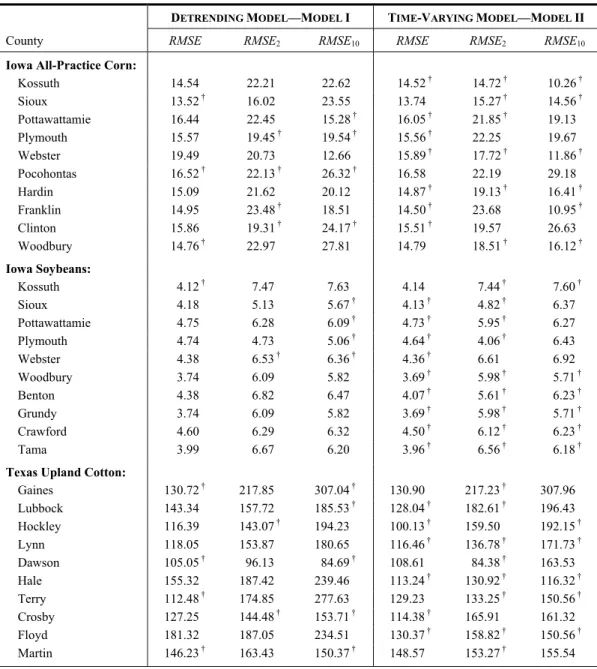
Table 3. Out-of-Sample Performance
DETRENDING MODEL—MODEL I TIME-VARYING MODEL—MODEL II
County RMSE RMSE2 RMSE10 RMSE RMSE2 RMSE10
Iowa All-Practice Corn:
Kossuth 14.54 22.21 22.62 14.52† 14.72 † 10.26† Sioux 13.52 † 16.02 23.55 13.74 15.27 † 14.56† Pottawattamie 16.44 22.45 15.28† 16.05† 21.85 † 19.13 Plymouth 15.57 19.45† 19.54† 15.56† 22.25 19.67 Webster 19.49 20.73 12.66 15.89† 17.72 † 11.86† Pocohontas 16.52 † 22.13† 26.32† 16.58 22.19 29.18 Hardin 15.09 21.62 20.12 14.87† 19.13 † 16.41† Franklin 14.95 23.48† 18.51 14.50† 23.68 10.95† Clinton 15.86 19.31† 24.17† 15.51† 19.57 26.63 Woodbury 14.76 † 22.97 27.81 14.79 18.51 † 16.12† Iowa Soybeans: Kossuth 4.12 † 7.47 7.63 4.14 7.44 † 7.60† Sioux 4.18 5.13 5.67† 4.13† 4.82 † 6.37 Pottawattamie 4.75 6.28 6.09† 4.73† 5.95 † 6.27 Plymouth 4.74 4.73 5.06† 4.64† 4.06 † 6.43 Webster 4.38 6.53† 6.36† 4.36† 6.61 6.92 Woodbury 3.74 6.09 5.82 3.69† 5.98 † 5.71† Benton 4.38 6.82 6.47 4.07† 5.61 † 6.23† Grundy 3.74 6.09 5.82 3.69† 5.98 † 5.71† Crawford 4.60 6.29 6.32 4.50† 6.12 † 6.23† Tama 3.99 6.67 6.20 3.96† 6.56 † 6.18†
Texas Upland Cotton:
Gaines 130.72 † 217.85 307.04† 130.90 217.23 † 307.96 Lubbock 143.34 157.72 185.53† 128.04† 182.61 † 196.43 Hockley 116.39 143.07† 194.23 100.13† 159.50 192.15† Lynn 118.05 153.87 180.65 116.46† 136.78 † 171.73† Dawson 105.05 † 96.13 84.69† 108.61 84.38 † 163.53 Hale 155.32 187.42 239.46 113.24† 130.92 † 116.32† Terry 112.48 † 174.85 277.63 129.23 133.25 † 150.56† Crosby 127.25 144.48† 153.71† 114.38† 165.91 161.32 Floyd 181.32 187.05 234.51 130.37† 158.82 † 150.56† Martin 146.23 † 163.43 150.37† 148.57 153.27 † 155.54
Note: † denotes a smaller out-of-sample predicted error in the two competing models.
(7)
( )
2 1 1 ˆ , n i i i RMSE Y Y n
where Yˆ( )i is the prediction for Yi obtained by fitting the model with observation i omitted. We sum the cross-validation errors and obtain the RMSE for the two competing models. As observed from table 3, the time-varying Beta distribution model outperforms the constant Beta model in most of the major agricultural production counties. Specifically, eight of the ten top Iowa corn production counties, nine of ten Iowa top soybean production counties, and six of seven Texas top cotton production counties exhibit a better cross-validation performance
in the time-varying model. The resulting RMSEs of the time-varying model for these yield data are smaller than those of the conventional model. The differences in the RMSE between the two competing models are larger for corn and cotton than soybeans. This finding is consistent with what we have observed in the practice of genetic improvement and bio-technological progress in agriculture. There have been fewer biotech innovations for soy-beans than for corn and cotton, and therefore the yield distribution of soysoy-beans is less affected. As a result, the two competing methods are not markedly different in their out-of-sample predictive power for soybean yields. In addition to computing RMSEs, one may also compute the Spearman’s correlation between the Yi’s and Ŷ(i)’s, or generate a Q-Q plot to check other distributional characteristics between the observed and (leave-one-out) predicted values.
In the current group risk crop insurance programs in the United States, yields are forecast two years into the future. These forecasts are then used to establish insurance guarantees. Accordingly, we considered an additional out-of-sample forecast evaluation, which was intended to provide an analog to the forecasts used in these area-wide programs. In this approach, models are ranked based on their out-of-sample forecasting performance for a series of two-year-ahead and 10-year-ahead forward forecasts. For example, to predict 1993’s yield, the estimates are based on the sample from 1926 to 1991; to predict 1994’s yield, the estimates are based on the sample from 1926 to 1992, etc. Another out-of-sample test is conducted by partitioning the entire sample into two parts and estimating parameters based on the first part of the data for the period 1926 to 1997 (the first 72 observations); then the estimated parameters are used to compute the expected (mean) yields for the out-of-sample period spanning 1998 to 2007 (the second part of the data). The mean of the squared differ-ence between the predicted value and the actual yield value is calculated as a “leave-10-out” forecast error (RMSE10).
The out-of-sample measures are computed for selected major crop/county combinations in the United States, and such predictive measures again provide comprehensive evidence that the time-varying approach represents an improvement across all criteria considered. Table 3 shows that time-varying model has smaller values of both RMSE2 and RMSE10 in most cases. Having noted this, we must point out that the out-of-sample comparison test is only based on the accuracy of first-moment mean prediction, which is not an overall evaluation of the entire yield distribution. Since the time-varying model is an alternative to the conventional two-stage model for estimating the yield distribution and forecasting the mean, these two models may display different out-of-sample performance based on different yield data with respect to mean prediction. Recall that strong evidence, as presented in table 2, supports the time-varying model’s performance in estimating the entire yield distribution in terms of likelihood-based tests and nonnested model distribution tests.
Table 4 presents alternative methods for comparing the two competing models. By using a regression method, we can consider which model’s predicted values better explain the variation of the actual yields. To this end, we regress actual yields on each of the alternative predictions. The results indicate that only the coefficient on predicted yields from the time-varying model is significantly different from zero, which suggests the time-time-varying model yields a better prediction of the actual yield. Further, the intercept term is also not signifi-cantly different from zero, indicating the chosen model has no systematic bias. Likewise, the coefficient on the time-varying model prediction is not significantly different from one, revealing that the chosen model has no scale bias.
Table 4. Other Model Comparison Methods
PANELA.COMPARED BY REGRESSION METHOD
Variable
Parameter
Estimate p-Value
Intercept −0.125 0.970
γ1: Coeff. of predictive value of detrended Beta −0.065 0.890
γ2: Coeff. of predictive value of time-varying Beta 1.068 0.034*
PANELB.RATE CROSS-VALIDATION
Description
Conventional Model
Time-Varying Model Mean of True Rates 0.0189 0.0058 Root Mean Squared Error (RMSE) 0.098 0.093 Mean Percentage Error (MPE) 1.66 0.45
Note: An asterisk (*) denotes statistical significance at the α = 0.10 or smaller level.
Simulation of a Group Risk Insurance Program
Yield-based insurance policies in the federal crop insurance program include the individual, farm-level multiple peril crop insurance (MPCI) and the county-level Group Risk Plan (GRP), which is based upon county-average yields from NASS. An important policy parameter in the GRP program is the premium rate, which is based on the county-average yield distribution. In this section, we evaluate the economic impacts of adopting rates based on the time-varying distribution methods. If the yield distributions change over time, premium rates should be adjusted accordingly. The premium rates from the proposed time-varying approach are illustrated with simulated data, and a rate cross-validation test is conducted to compare the predictive accuracy of the premium rates from the time-varying approach with those of the conventional two-stage approach (table 4). Standard crop yield insurance pays an indemnity at a predetermined price to replace yield losses. Under the GRP, insured farmers collect an indemnity if the county average yield falls beneath a guarantee, regardless of the farmers’ actual yields. Loss probabilities correspond to the likelihood that yields y below some threshold will be observed, which is given by the area under the density curve to the left of the guaranteed yield.
Consider an insurance contract that insures some proportion (λ(0,1)) of the expected crop yield (ye). If y < λye, the insurer will pay (λye – y)p as an indemnity, where p is a predetermined price. An actuarially fair premium is defined by the expected loss of this contract, which takes the following form:
(8) E Loss( )E(yey I y) ( ye)p E (yey)p,
where a+ = max(0, a) for a number a . In the preceding discussion, y denotes the observed annual county-level yield, and ye represents the predicted (guaranteed) yield. Calculation of expected loss requires estimation of the distribution of yields. We compare the conventional two-stage estimation method to the proposed time-varying distribution in terms of expected loss and premium rates.
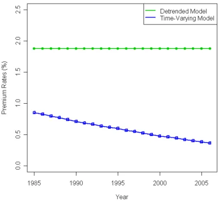
Figure 4. Premium rates (75% coverage-level crop insurance contract) for time-varying model and detrended model (1985–2006)
In our simulation, one million yields are generated from the time-varying Beta distributions. The probability of yield loss, the expected yield loss, and the actuarially fair premium rate associated with a contract that guarantees 75% of the expected yield is calculated for each year. As shown in figure 4, the premium rates range from 0.83% in 1985 to 0.36% in 2006 for the case in which the yields are from the time-varying model. The rates change as the moments of the time-varying distribution evolve. In contrast, the premium rates calculated from a conventional two-stage Beta distribution model (model I) indicate a constant premium rate around 1.88% from 1927 to 2006. For crop insurance in 2006, the premium rate from the detrended Beta model is 1.52 percentage points higher than the premium from the time-varying Beta model (0.36% versus 1.88%). Thus, the conventional model tends to signifi-cantly overprice the same level of coverage.
Rate cross-validation is proposed to measure the predictive accuracy of premium rates of one model when the alternative model is true. Rate cross-validation can be tested as follows: ■ STEP 1. Assume one of the alternative yield distribution models (denoted by j) is true,
and simulate a set of actuarially fair premium rates (denoted as rtruej,t).
■ STEP 2. Simulate 1,000 sets of 80 pseudo-observations of corn yields from the
corres-ponding true yield distribution.
■ STEP 3. Obtain 1,000 sets of MLEs based on these pseudo-observations; then calculate the “pseudo” actuarially fair premium rates (denoted as rj′,t) based on the MLEs.
We can then compare the pseudo-premium rates with the true rates and obtain the mean percentage error (MPE) and the root mean squared error (RMSE).
Cross-validation demonstrates a smaller MPE and RMSE for the time-varying model. As is shown in table 4 (panel B), when the true rate is derived from the conventional model (with an average rate equal to 0.0189), the root mean squared error (RMSE) of predicted rates of the time-varying model is 0.093. This RMSE of predicted rates is 5.10% lower than the RMSE (0.098) obtained from the conventional model when the alternative (the average premium rate implied by the time-varying model is 0.0058) is true. In addition, the MPE is 0.45 for the time-varying model and 1.66 for the detrended model. Smaller MPE and RMSE values confirm that the time-varying model is more accurate, flexible, and robust in terms of premium rate prediction. This prediction error can also be expressed in economic terms. For example, for a crop insurance contract with $1,000 liability per acre, the rate cross-validation error of the premium is $8.68 for the time-varying model. The rate cross-validation error of the premium is $9.60 for the conventional model. Therefore, the predicted premium error of the time-varying model is $0.92 less than the detrended model per unit of insurance ($1,000 of total liability in this example). In light of the fact that the total premium in the federal crop insurance program in 2009 was nearly $80 billion, pricing errors can result in substantial aggregate losses. Consequently, the accuracy of insurance rates is improved by applying the time-varying yield distribution model.
Conclusions
This study has examined the accuracy of alternative methods for measuring conditional yield risk under technological change. We propose a method for incorporating trends in the yield distribution that may offer a more accurate and consistent method for estimating the distribu-tion of crop yields than other approaches commonly used in the literature. Because this method involves simultaneously estimating the time trend effects and the parameters of the yield distribution, it therefore overcomes possible shortcomings associated with the more common approach of treating the detrended yields as “observed” data rather than data estimated from a previous detrending model. Several model selection tools are used to compare the in-sample goodness of fit and out-of-sample predictive power of the alternative models. The results show that the proposed time-varying model is superior to the conventional two-stage model in terms of providing a better fit (i.e., lower AIC and BIC criteria) and stronger out-of-sample predictive power for most of the major county/crop combinations. The results of out-of-sample prediction tests are consistent with prior expectations based on technological progress and biotechnology. In particular, multiple biotech traits and genetic improvements have emerged for corn and, to a lesser degree, for cotton. Many biotech innovations for soy-beans have involved herbicide tolerance. The proposed time-varying method therefore appears to offer greater improvement for corn and cotton than is the case for soybeans.11
In a rate simulation exercise, the premium rate derived from the time-varying model showed significantly decreasing premium rates (from 0.83% in 1985 to 0.36% in 2006) over time, while the conventional model implied a constant rate (1.88%). A method of “rate cross-
11 A referee has astutely pointed out that the time-varying model may have advantages when applied to such a long span of data (1927–2009) because of its greater flexibility. GRP and GRIP insurance contracts are based on a much shorter series of data (typically dating from 1958). We repeated the analysis using shorter series (1958–2009 and 1973–2009) and reached very similar conclusions, which supported the advantages of the time-varying approach. These results are available from the authors upon request.
validation” demonstrated that the time-varying distribution model may offer significant advantages, even when the underlying yield trend process is misspecified. Overall, this analysis reveals a dynamic evolution of yield distributions under technological change for major U.S. crop yields. In our data, which represent county-level yields for important crops in major growing areas, we find that the time-varying model provides a superior fit to the data.
This study has policy implications that relate to improving the accuracy of assessing yield distributions in cases where parameters of the distribution evolve over time. When distri-butions change, premium rates can be adjusted to represent the most recent information. This offers the potential to improve the accuracy of models used in rating crop insurance contracts and may improve risk-management mechanisms to protect producers from risk. The improved time-varying method has practical implications for the GRP and GRIP programs as well as the design of other insurance contracts. Our applications assume a Beta distribution for each year. Future research may benefit from relaxing this assumption by using more flexible models such as a mixture of Beta distributions and nonparametric methods.
[Received November 2009; final revision received December 2010.]
References
Akaike, H. “A New Look at Statistical Model Identification.” IEEE Transactions on Automatic Control
19(1974):716–723.
Atwood, J. A., S. Shaik, and M. J. Watts. “Are Crop Yields Normally Distributed? A Re-examination.”
Amer. J. Agr. Econ. 85,4(2003):888–901.
Burnham, K. P., and D. Anderson. Model Selection and Multi-Model Inference. New York: Springer, 2003. Chen, S. L., and M. Miranda. “Modeling Multivariate Crop Yield Densities with Frequent Extreme Events.”
Paper presented at AAEA annual meeting, Denver, CO, August 2004.
Day, R. H. “Probability Distributions of Field Crops.” J. Farm Econ. 47(August 1965):713–741.
Goodwin, B. K., and A. P. Ker. “Nonparametric Estimation of Crop Yield Distributions: Implications for Rating Group-Risk (GRP) Crop Insurance Contracts.” Amer. J. Agr. Econ. 80(1998):139–153.
Gyorfi, L., M. Kohler, A. Krzyzak, and H. Walk. A Distribution-Free Theory of Nonparametric Regression. New York: Springer, 2002.
Just, R. E., and Q. Weninger. “Are Crop Yields Normally Distributed?” Amer. J. Agr. Econ. 81(1999): 287–304.
Miranda, M. J., and J. W. Glauber. “Systemic Risk, Reinsurance, and the Failure of Crop Insurance Markets.”
Amer. J. Agr. Econ. 79(1997):206–215.
Nelson, C. “The Influence of Distribution Assumptions of the Calculation of Crop Insurance Premia.” N. Cent. J. Agr. Econ. 12(1990):71–78.
Nelson, C., and P. Preckel. “The Conditional Beta Distribution as a Stochastic Production Function.” Amer. J. Agr. Econ. 71,2(1989):370–378.
Ozaki, V. A., S. K. Ghosh, B. K. Goodwin, and R. Shirota. “Spatio-Temporal Modeling of Agricultural Yield Data with an Application to Pricing Crop Insurance Contracts.” Amer. J. Agr. Econ. 90,4(2008):951–961. Ramirez, O. “Estimation and Use of a Multivariate Parametric Model for Simulating Heteroskedastic,
Correlated, Nonnormal Random Variables: The Case of Corn Belt Corn, Soybean, and Wheat Yields.”
Amer. J. Agr. Econ. 79(1997):191–205.
Ramirez, O., S. Misra, and J. Field. “Crop-Yield Distributions Revisited.” Amer. J. Agr. Econ. 85,1(2003): 108–120.
Robinson, P. “Asymptotically Efficient Estimation in the Presence of Heteroskedasticity of Unknown Form.”
Schwarz, G. “Estimating the Dimension of a Model.” Annals of Statis. 6(1978):461–464.
Sherrick, B., F. Zanani, G. Schnitkey, and S. Irwin. “Crop Insurance Valuation Under Alternative Yield Distribution.” Amer. J. Agr. Econ. 86,2(2004):406–419.
Swinton, S., and R. King. “Evaluating Robust Regression Techniques for Detrending Crop Yield Data with Non-Normal Errors.” Amer. J. Agr. Econ. 73(1991):446–461.
Taylor, C. “Two Practical Procedures for Estimating Multivariate Nonnormal Probability Density Functions.”
Amer. J. Agr. Econ. 72(1990):210–217.
Vuong, Q. H. “Likelihood Ratio Tests for Model Selection and Non-nested Hypotheses.” Econometrica
57(1989):307–333.
Wilks, S. “The Large-Sample Distribution of the Likelihood Ratio for Testing Composite Hypotheses.”