Efficient Estimators for Adaptive Two-Stage Sequential Sampling

0.8 Cop yedited by: AA 1 2 3 4 5 6 7 8 9 10 11 12 13 14 15 16 17 18 19 20 21 22 23 24 25 26 27 28 29 30 31 32 33 34 35 36 37 38 39 40 41 42 43 44 45 46 47 48 49 50

Vol. 00, No. 0, Month 2009, 1–17

Efficient estimators for adaptive two-stage sequential sampling

a_{Department of Mathematical Sciences, Isfahan University of Technology, Isfahan, Iran;}b_{Department of}

Mathematics and Statistics, University of Canterbury, Private Bag 4800, Christchurch, New Zealand;

c_{Leetown Science Center, US Geological Survey, 11649 Leetown Road, Kearneysville, WV 25430, USA Q1}

(Received 16 January 2009; final version received 29 April 2009)

In stratified sampling, methods for the allocation of effort among strata usually rely on some measure of within-stratum variance. If we do not have enough information about these variances, adaptive allocation can be used. In adaptive allocation designs, surveys are conducted in two phases. Information from the first phase is used to allocate the remaining units among the strata in the second phase. Brownet al.[Adaptive two-stage sequential sampling, Popul. Ecol. 50 (2008), pp. 239–245] introduced an adaptive allocation sampling design – where the final sample size was random – and an unbiased estimator. Here, we derive an unbiased variance estimator for the design, and consider a related design where the final sample size is fixed. Having a fixed final sample size can make survey-planning easier. We introduce a biased Horvitz– Thompson type estimator and a biased sample mean type estimator for the sampling designs. We conduct two simulation studies on honey producer in Kurdistan and synthetic zirconium distribution in a region on the moon. Results show that the introduced estimators are more efficient than the available estimators for both variable and fixed sample size designs, and the conventional unbiased estimator of stratified simple random sampling design. In order to evaluate efficiencies of the introduced designs and their estimator furthermore, we first review some well-known adaptive allocation designs and compare their estimator with the introduced estimators. Simulation results show that the introduced estimators are more efficient than available estimators of these well-known adaptive allocation designs.

Keywords: stratified population; Neyman’s allocation; Horvitz–Thompson type estimator; sample mean

type estimator Q2

AMS Subject Classification: 62D05; 92-08

1. Introduction

In conventional stratified sampling, the population is partitioned into regions or strata, and a simple random sample is selected in each stratum, with the selections in one stratum being independent of selections in the others. To obtain the best estimate of the total population with a given total Q3

sample size or total survey cost, or to achieve a desired precision with minimum cost, optimal allocation of sample size among the strata is necessary, which results in larger sample sizes in strata that are larger, more variable and less costly to sample [1,2].

*Corresponding author. Email: [email protected]

ISSN 0094-9655 print/ISSN 1563-5163 online © 2009 Taylor & Francis

DOI: 10.1080/00949650903005664 http://www.informaworld.com

51 52 53 54 55 56 57 58 59 60 61 62 63 64 65 66 67 68 69 70 71 72 73 74 75 76 77 78 79 80 81 82 83 84 85 86 87 88 89 90 91 92 93 94 95 96 97 98 99 100

If prior knowledge of the strata variances is not available, it would be natural to carry out the sampling in two phases and compute sample variances from the first phase, which are then used to adaptively allocate the remaining sample size among strata. Alternatively, allocation of the remaining sample size could be based on the stratum–sample mean or on the number of large values in the first-phase sample rather than sample variances, since with many natural populations high means or large values are associated with high variances. The standard stratified sampling estimator gives an unbiased estimator of the total population with conventional stratified random sampling, but it is not in general unbiased with adaptive allocation designs.

Francis [3] introduced an adaptive allocation method in stratified sampling. Francis suggested to select 75% of the final sample size by SRS, and then allocate the remaining sample among

Q4

strata. In this method, the variances of estimators are estimated from the first-phase sample. Then, one unit is added to the stratum with the largest decrease in the variance. On the basis of the new sample set, the variance is estimated, and the second unit is selected from the stratum with the largest decrease in the variance. This process is continued to allocate the remaining units.

Jolly and Hampton [4] proposed another adaptive allocation. Their method is similar to Francis’s method. At first, approximately 75% of the final sample size are selected and sample variances are estimated for all strata, and then, by Neyman’s method, the remaining units are allocated to strata. They applied their method to an acoustic survey of South African anchovy.

Salehi and Smith [5] introduced two-stage sequential sampling. In the special case that all primary units are selected, the sampling design may be considered as an adaptive allocation sample design. In the first phase, a simple random sample is selected from each primary sample unit (stratum). To conduct the second phase, a condition C is defined for which the remaining sample size is allocated based on the value of the variable of interest. They used Murthy’s estimator, which is an unbiased estimator, for the population mean.

Brown et al.[6] introduced an adaptive allocation with variable sample size design. The first phase is conducted similar to the first phase in Salehi–Smith’s design. A multiplierdis considered before sampling. In the second phase, iflh1units from the first phase sample in stratumhsatisfied the conditionC, then additionald ×lh1units are sampled from the remaining units in stratumh. They used Murthy’s estimator to estimate the population mean.

In Section 2, we describe Brownet al.’s adaptive allocation sampling design and introduce a fixed sample size version. We also describe Francis’s design, Jolly–Hampton’s design, and Salehi– Smith’s design. In Section 3, we derive an unbiased variance estimator for Brownet al.[6]. Two biased estimators are introduced for the variable and fixed sample size designs. We then study their sampling properties analytically. In Section 4, two empirical studies using honey producer population in Kurdistan and synthetic zirconium distribution population in a region on the moon, are described.

2. Sampling designs

Suppose that we have a population ofN units which are partitioned intoH strata of sizeNhunits (h=1, . . . , H ). Let unithidenote theith unit in thehth stratum with an associated measurement or countyhi, andKhis the number of units satisfying a conditionCin thehth stratum. The condition C for unithi is defined as (yhi > c).

Suppose that variances of strata are unknown and we have no prior information on variances’ estimator of strata. Therefore, Neyman’s allocation cannot be used. We describe two adaptive allocation sampling designs, one with a variable sample size [6] and the other with a fixed sample size. We also describe adaptive allocation designs introduced by Francis [3], Jolly and Hompton [4], and Salehi and Smith [5] in this section.

101 102 103 104 105 106 107 108 109 110 111 112 113 114 115 116 117 118 119 120 121 122 123 124 125 126 127 128 129 130 131 132 133 134 135 136 137 138 139 140 141 142 143 144 145 146 147 148 149 150

2.1. Variable sample size design

In the variable sample size design, initially a first phase sample of sizenh1 units is taken without replacement from each stratum wheren1 =PH_h=1nh1 is the total sample size of the first phase. In this paper we assume that we have no prior information about the strata variances, then in the variable sample size design and next designs we allocate a fixednh1 to all strata proportional to stratum size. If lh1 units of the first phase sample units in the hth stratum satisfy the condition

C, d×lh1 additional sample units are selected without replacement from the remaining units in stratumh. The multiplierdis chosen prior to sampling. Because sampling is without replacement in either phases, anddis a fixed multiplier in all strata, the following inequality can be imposed:

0< d ≤ min ½ Nh−nh1 lh1 |h=1, . . . , H ¾ .

Whennh1+d×lh1 is larger thanNh, we select all units in stratumhand we can, therefore,

ignore the above restriction similar to Neyman’s allocation.

In this designn2 =dPH_h=1lh1, the number of adaptively added units, and, therefore, the final

total sample size,n=n1+n2, are random. This implies that

d = n_P−n1

hlh1 ,

wherenin this design is random. However, by fixingnprior to sampling, this relationship can be used to determinedunder a fixed sample size version of the design.

2.2. Fixed sample size design

A variable sample size can make it difficult to plan and implement sampling. By setting the sample size prior to sampling and using the results from the first phase of sampling, a fixed sample size design can be introduced. Suppose that we fix the final sample size at n, and select a random sample of sizenh1 without replacement from each of the strata. Thend will be bounded and is given by

d = n_P−n1

hlh1 .

We can select d×lh1 units from stratumh when Phlh1 >0. In the fixed sample size design, if P_hlh1 >0 the final sample size would be equal to the predetermined sample size n, but if

P

hlh1 =0, multiplierd is undefined. To achieve fixed sample sizen, we allocate the remaining

n−P_hnh1units equally to strata whenP_hlh1 =0.

We should note that attaining the predetermined sample size n is not strictly true because

n1+P_hd ×lh1 may not be a whole number. For example, consider this case where we want

n=20 and we have a population of three equal-sized strata. We start off withn1 =9. The three strata are sampled in the first phase by selecting three units in each, and we find lh1 =2 in the first strata, 2 in the second and 1 in the third. The multiplier would be calculated as d =

(20−9)/(2+2+1)=11/5=2.2. We then select in the second phase 2.2×2=4.4 which we round to 4 units in the first stratum, 4 in the second and 2 in the third. Our final sample size is 9+4+4+2=19 and not 20. The final sample size will be approximately equal to the predetermined sample size and may vary by a small amount depending on the effect of converting the real numbers to integers.

151 152 153 154 155 156 157 158 159 160 161 162 163 164 165 166 167 168 169 170 171 172 173 174 175 176 177 178 179 180 181 182 183 184 185 186 187 188 189 190 191 192 193 194 195 196 197 198 199 200 2.3. Francis’s design

Francis [3] in his fisheries research allocated fixed sample size nto the strata in two phases. In the second phase, sampling was carried out in a sequential fashion. Francis’s design is based on variance estimate of total weight of fish (biomass) in the first phase in stratum h. When we estimate the stratum total parameter by conventional estimator, we used Francis’s design with little modification, as shown in the following. In the first phase, units are selected similar to the variable design. In this method to allocate remainingn−PH_h=1nh1 units, we should follow the following steps for each unit. If an additional unit is added to stratum h, then, using the same estimates_h2₁from the first phase, the reduction in the estimated variance of the conventional estimator is Gh =Nh2 µ ₁ nh1 − 1 nh1+1 ¶ s_h2₁ = N 2 hs 2 h1 nh1(nh1+1) .

This formula is now used to determine phase-2 allocations sequentially. The first unit of the remaining units is allocated to the stratum for whichGhis the greatest. Suppose that this is stratum j. Then Gj is recalculated as sj21/(nj1+1)(nj1+2). The next unit is added to the stratum for whichGhis a maximum, and so on.

2.4. Jolly–Hampton’s design

Jolly and Hampton’s adaptive allocation sampling design can be formulated as a fixed sample size design. In Jolly–Hampton’s design,nh1units has been selected from each stratum as previous designs. Suppose that the final sample size is fixed atn. A first phase sample of sizenh1is selected without replacement from stratum hsuch thatnh1 < n/H. Then the remainingn−n1 units are allocated as follows. Variances of strata are then estimated from the first phase sample. The sample size in thehth stratum is computed by

nh =nh1 +(n−n1)

Nhsh1

PH

h=1Nhsh1

,

wheresh1is the standard deviation of the first phase sample in the stratumh.

If sample size in thehth stratum is larger thanNh, we select all units in stratumh.

2.5. Salehi–Smith’s design

Salehi–Smith’s two-stage sequential sampling is an adaptive allocation sampling design when all primary sampling units are selected in the first phase. It can be formulated as a variable sample size design. In the first phase, a simple random sample ofnh1units is drawn without replacement from stratumh(h=1, . . . , H ). If conditionC is satisfied for at least one unit in thehth stratum in the first phase sample, a predetermined number of additional units, say nh2, are selected at

random from the remaining units in stratum h. As a result n=P_hnh1+Phnh2 =n1+n2 is the sample size and is a random value.

2.6. Comparison of variable and fixed sample size designs

The variable sample size design and the Salehi–Smith’s design share an advantage over the other two designs, in that the allocation of second phase effort can be done during the first phase. The fixed sample size design, the Francis design, and the Jolly–Hampton design all require the first phase to be completed and strata to be visited before second phase allocation can occur. This

201 202 203 204 205 206 207 208 209 210 211 212 213 214 215 216 217 218 219 220 221 222 223 224 225 226 227 228 229 230 231 232 233 234 235 236 237 238 239 240 241 242 243 244 245 246 247 248 249 250

means that stratum that is to be surveyed in the second phase will need to be revisited, and this may be costly.

Conversely, the variable sample size design and the Salehi–Smith’s design share a disadvantage over the other designs in that the final sample size is not known prior to surveying. This can make planning the survey difficult. With the fixed sample size design, the Francis design, and the Jolly–Hampton design, the size of the final sample is known.

3. Estimations

Let τh =PNi=h1yhi be the total of y values in the hth stratum, and τ =PHh=1τh be the total

population. To estimateτ and var(τ )ˆ , we estimateτhandvar(τˆh). We then have

ˆ τ = H X h=1 ˆ τh c var(τ )ˆ = H X h=1 c var(τˆh).

We will derive Murthy’s estimator for the variable sample size design [6], and two biased estimators for both fixed and random sample size designs. The first biased estimator – the Horvitz– Thompson type estimator (τˆHT) – is the HT estimator for which the inclusion probabilities are estimated. The HT estimator is an unbiased estimator but the inclusion probabilities depend on the parameters of population for the introduced sampling designs. We, therefore, estimate the inclusion probabilities, so thatτˆHTis a biased estimator. The second biased estimator is the sample mean type estimator.

3.1. Murthy’s estimator in the variable sample size design

Brownet al. [6] introduced Murthy’s estimator for the variable sample size design, which is an unbiased estimator ˆ τMh = n X i=1 P (S_h|i) P (S_h) yhi =Nh[ ˆphy¯ch+(1− ˆph)y¯c0h].

We derive its variance estimator, which is given by

var(τˆMh)= Nh X i=1 Nh X j <i  1− X S_h3i,j P (S_{h|i)P (}S_{h|j )} P (S_h)  (yhi −yhj)2,

whereP (S_{h)is the probability of getting sample} S_{h, P (}S_{h|i) is the conditional probability of}

getting the sampleS_{h, given theith unit was selected first,y¯chandy¯c}0_hare respectively the mean of units satisfying the conditionCand not satisfying the conditionCin strationh, andpˆh =lh1/nh1.

It can be shown that, using Rao–Blackwell method, this estimator is an improved estimator and it is a function of minimal sufficient statisticsS_{h, where}S_{his the observed unordered set of}

distinct units in the sample.

From the Rao–Blackwell theorem var(τˆMh)=var(y¯h1)−E(var(y¯h1)|Sh) and varc(τˆMh)= c

251 252 253 254 255 256 257 258 259 260 261 262 263 264 265 266 267 268 269 270 271 272 273 274 275 276 277 278 279 280 281 282 283 284 285 286 287 288 289 290 291 292 293 294 295 296 297 298 299 300

With routine but lengthy algebra,var_c[ ˆτMh]is simplified as follows: c var(τˆMh)=Nh ½ ˆ ph · (Nh−1)(lh1 −1) nh1−1 + µ (Nh−nh1)(1− ˆph) nh1−1 −Nhpˆh ¶ lh−1 lh ¸ s_ch2 + ˆph(1− ˆph) Nh−nh1 nh1−1 (y¯ch− ¯yc0_h)2+(1− ˆp_h) × · (Nh−1)(nh1−lh1−1) nh1−1 + µ (Nh−nh1)pˆh nh1−1 −Nh(1− ˆph) ¶ l_h0 −1 l_h0 ¸ s_c20_h ¾ ,

where S_{ch and} S_c0_h are, respectively, the subsamples of units satisfying the condition C and the subsamples of units not satisfying the condition C in stratumh, lh andlh0 are, respectively,

the cardinality of these subsamples in stratum h, s_ch2 =1/(lh−1)P_i∈S_ch(yhi− ¯ych)

2_{, s}2

c0_h= 1/(l_h0 −1)P_i∈S

c0h(yhi− ¯yc 0_h)2.

Brownet al.[6] showed that this estimator is efficient than the estimator for a very rare popula-tion. We should note that using Rao–Blackwell method would improve the estimator more when the second phase sample is more consistent with the first phase sample.

3.2. Horvitz–Thompson type estimator

3.2.1. Horvitz–Thompson type estimator in variable sample size design

Horvitz and Thompson [7] introduced an unbiased estimator for the total population, which we can apply it for estimatingτh as

ˆ τHTh= X i∈S_h yhi πhi ,

whereπhi is the inclusion probability of the hith unit in the sample. In the introduced variable

sample size design,πhi is given by

πhi =                                                                      nh1 X lh1=1 Ã Kh−1 lh1−1 ! Ã Nh−Kh nh1 −lh1 ! Ã Nh−nh1 d ×lh1 ! + Ã Kh−1 lh1 ! Ã Nh−Kh nh1 −lh1 ! Ã Nh−nh1 −1 d ×lh1−1 ! Ã Nh nh1 ! Ã Nh−nh1 d ×lh1 ! , i∈S_ch, nXh1−1 lh1=0 Ã Kh lh1 ! Ã Nh−Kh−1 nh1−lh1−1 ! Ã Nh−nh1 d×lh1 ! Ã Nh nh1 ! Ã Nh−nh1 d×lh1 ! + nh1 X lh1=1 Ã Kh lh1 ! Ã Nh−Kh−1 nh1−lh1 ! Ã Nh−nh1−1 d×lh1 −1 ! Ã Nh nh1 ! Ã Nh−nh1 d×lh1 ! , i∈S_c0_h,

301 302 303 304 305 306 307 308 309 310 311 312 313 314 315 316 317 318 319 320 321 322 323 324 325 326 327 328 329 330 331 332 333 334 335 336 337 338 339 340 341 342 343 344 345 346 347 348 349 350

which can be simplified as

πhi =        nh1 Nh µ 1+d µ Kh−1 Nh−1 ¶¶ ifi ∈S_ch, nh1 Nh µ 1+d µ Kh Nh−1 ¶¶ ifi ∈S_c0_h,

whereKhis the number of units satisfying the conditionCin stratumh. It cannot be calculated,

givenS_{. Inclusion probabilityπhi depends on parameterKh. Christman [8] introduced adaptive}

two-stage one-per-stratum sampling in which she used the same HT estimator for estimating its component. Her empirical study showed that the introduced estimator is efficient.

We use unbiased and consistent estimatorKˆh =Nhlh1/nh1 inπhi. We then have

ˆ τh= X i∈S_h yhi ˆ πhi , where ˆ πhi =              nh1 Nh à 1+d à ˆ Kh−1 Nh−1 !! ifi ∈S_ch, nh1 Nh à 1+d à ˆ Kh Nh−1 !! ifi ∈S_c0_h.

The variance estimator is given by

c var(τˆHTh)= X i∈S X j∈S µ πij πiπj −1 ¶ yiyj πij ,

whereπij is the joint inclusion probability which is given by

πij =                                                    nh1(nh1−1) Nh(Nh−1) ½ 1+ d nh1 −1 µ 2+ (2nh1−3)(Kh−2) Nh−2 +d(Kh−2) (Nh−2)2 · (Nh−Kh)(Nh−nh1−2) Nh−3 +nh1(Kh−2) ¸¶¾ ifi, j ∈S_ch, nh1(nh1−1) Nh(Nh−1) ½ 1+ d nh1 −1 µ 1+ (2nh1−3)(Kh−1) Nh +d(Kh−1) (Nh−2)2 · (Nh−Kh−1)(Nh−nh1−2) Nh−3 +nh1(Kh−1) ¸¶¾ ifi ∈S_ch, j ∈S_c0_h, nh1(nh1−1) Nh(Nh−1) ½ 1+ d nh1 −1 µ (2nh1−3)Kh Nh + dKh (Nh−2)2 · (Nh−Kh−2)(Nh−nh1 −2) Nh−3 +nh1Kh ¸¶¾ ifi, j ∈S_c0_h.

351 352 353 354 355 356 357 358 359 360 361 362 363 364 365 366 367 368 369 370 371 372 373 374 375 376 377 378 379 380 381 382 383 384 385 386 387 388 389 390 391 392 393 394 395 396 397 398 399 400

3.2.2. Horvitz–Thompson type estimator in fixed sample size design

Inclusion probability in fixed sample size design is more complicated because multiplierdis not fixed before completing the first phase. It depends on the number of sample units satisfying the condition C in the first phase. We now estimate the inclusion probability in fixed sample size design with respect to variableD.

For fixed sample size, designD is as follows:

D =            n−n1 P hlh1 if X h lh1 ∈ {1,2, . . . , n1}, n−n1 H if X h lh1 =0. π_hi0 =X S3i P (S₎₌X S3i X d P (S_{, D =d)=}X d P (D=d)X S3i P (S_{|D =d).}

We know from the previous design that the second summation in the above equation is the inclusion probability in the variable sample size design, so that

π_hi0 =X d P (D =d)πhi =            X d P (D =d)nh1 Nh µ 1+dKh−1 Nh−1 ¶ i ∈S_ch, X d P (D =d)nh1 Nh µ 1+d Kh Nh−1 ¶ i ∈S_c0_h. =          nh1 Nh µ 1+E(D)Kh−1 Nh−1 ¶ i ∈S_ch, nh1 Nh µ 1+E(D) Kh Nh−1 ¶ i ∈S_c0_h.

To calculateE(D)we need to have probability function ofD, where it is

P (D =d)=      P µ P hlh1 = n−n1 d ¶ ifd 6= n−n1 H , P (P_hlh1 =0) ifd = n−n1 H . P Ã X h lh1 =l. ! = X l1,...,lH−1 P (l1, l2, . . . , lH−1, l.−l1−l2− · · · −lH−1) = X l1,...,lH−1 P (l1)P (l2)· · ·P (lH−1)P (l.−l1−l2 − · · · −lH−1) = X l1,...,lH−1 µ k1 l1 ¶ µ N1−K1 nh1−l1 ¶ µ N1 nh1 ¶ . . . × µ KH l.−l1− · · · −lH−1 ¶ µ NH −KH nhH −(l.−l1− · · · −lH−1) ¶ µ NH nhH ¶

401 402 403 404 405 406 407 408 409 410 411 412 413 414 415 416 417 418 419 420 421 422 423 424 425 426 427 428 429 430 431 432 433 434 435 436 437 438 439 440 441 442 443 444 445 446 447 448 449 450

The probability function ofDdepends on the population parameters, and calculatingE(D)from the sample is impossible. To solve the problem we recommend to replace the unbiased estimator

DwithE(D). With this substitution, equation of inclusion probabilities in both variable and fixed sample size design will be identical.

3.3. Sample mean type estimator of total WhenNhis large, we have

lim Nh→∞ dnh1 Nh(Nh−1) =0. Thus lim Nh→∞(τˆh)=Nlimh→∞ µ y.ch nh1/Nh+dlh1/(Nh−1)−dnh1/Nh(Nh−1) + y.c0h nh1/Nh+dlh1/(Nh−1) ¶ ∼ = y.ch+y.c0h (nh1+dlh)/Nh =Nhy¯hs,

wherey.chandy.c0_hare, respectively, the total of units satisfying the conditionCand not satisfying

C. We, therefore, can use estimatorτˆs =PhNhy¯hs, whenNhs are relative large. It is clear thatτˆs

is another biased estimator which can be computed easily. WhenNhis large, the sample mean and

HT type estimator are approximately equal but whenNhis small they can be different estimators.

In the appendix, we show thatτˆs is a negatively biased estimator.

4. Simulation study

In this section, the efficiency of the five sample designs are investigated using two populations. The first population is honey producer in Kurdistan Province of Iran (HPK) [9], and the second simulated population synthetic zirconium in a region on the Moon (SZM) [10]. Since we did not have access to the value of units not satisfying conditionC we simulate them. The results for both populations are almost similar but we present both to illustrate the versatility of the sampling designs. We also want to use the most recently used populations rather than the most frequent populations in this context. The maps of HPK and SZM are shown in Figures 1 and 2, respectively. In population HPK, cities or villages are sampling units of which there were 1864. We partitioned the map of Kurdistan province into four strata, each containing 466 units. The units in each strata have approximately the same geographical condition. We are interested in the variable yi, the

amount of produced honey in unitiin a year. We defined the conditionC (yi >20)which can be

considered as active units in producing honey. In HPK,Kh is 0,1,15, and 39 in the four strata.

For the SZM population [10], the region of the moon is partitioned into 560 equal-sized units and synthetic zirconium is measured in each. The region is stratified into eight strata. The condition is defined asyi ≥ 1. In SZM,Khis 3,0,11,0,22,0,9, and 0 in the eight strata.

We use the five sample designs introduced in Section 2 and compare the efficiency of designs with different estimators (Section 3) by Monte Carlo simulation. We use 30,000 replicate samples for each design and estimator combination. Efficiency was estimated by comparing the design and estimator combination with stratified simple random sampling using the same sample size within each stratum. We estimate the relative bias of introduced biased estimators in the five introduced sample designs by the Monte Carlo simulation.

For the variable sample size design, the set of first phase sample sizes in each stratum was

451 452 453 454 455 456 457 458 459 460 461 462 463 464 465 466 467 468 469 470 471 472 473 474 475 476 477 478 479 480 481 482 483 484 485 486 487 488 489 490 491 492 493 494 495 496 497 498 499 500

Figure 1. The shaded in region black on the map is Kurdistan province of Iran that is partitioned to four strata and numbers show the strata.

Figure 2. Lunar Orbiter photograph III-133-H2 of prospecting region north of Apollo 14 landing site (photograph courtesy of Lunar and Planetary Institute). Bold numbers in the two besides are the strata numbers.

design, the Francis design, and for the Jolly–Hampton’s design, the final sample size was selected so that it equalled the effective sample size for all pairs of nh1 and d from the variable sample size design. For the Salehi–Smith’s design, we selectedn2such that the effective sample size was matched with the effective sample size for all pairs of nh1 and d from the variable sample size design.

501 502 503 504 505 506 507 508 509 510 511 512 513 514 515 516 517 518 519 520 521 522 523 524 525 526 527 528 529 530 531 532 533 534 535 536 537 538 539 540 541 542 543 544 545 546 547 548 549 550

The sample mean type estimator was used for all five designs. In addition, the HT type estimator was used for the variable and fixed sample size design, and Murthy’s estimator for the variable sample size design, for the fixed sample size design and for the Salehi–Smith’s design (see [5] for details of Murthy’s estimator).

For each combination of designs and estimator we calculated

MSE[ ˆτ?] = 1 29999 30000_X i=1 (τˆ?− ¯τ?)2+(τ¯?−τ )2,

whereτ¯? =1/30000P30000_i=1 τˆi?. We have used the notationτˆ?, which stands forτˆM,τˆHT,τˆs, where

ˆ τM = P hτˆMh,τˆHT= P hτˆh, andτˆs = P hNhy¯hs.

The relative efficiency ofτˆ?is given by

eff[ ˆτ?] =

VAR[ ˆτst]

MSE[ ˆτ?]

×100.

For each combination of designs and biased estimators for HPK we calculated

RB(τˆ?)=

¯

τ?−τ τ

whereτˆ?stands forτˆHT andτˆs.

Results are summarized in Tables 1–3, and in Figures 3–8, where e.s.s, v.d, f.d, Fr.d, J.d and S.d are used as abbreviations of effective sample size design, variable sample size design, fixed sample size design, Francis’s design, Jolly–Hampton’s design and Salehi–Smith’s design.

In Figures 3– 8, the efficiency of estimators for the variable designs (v.d and S.d), fixed designs (f.d, Fr.d, and J.d), and the best estimators in the variable and fixed designs for two populations are plotted. From Tables 1 and 2, we can see the efficiency of the sample mean type and HT type for

Table 1. Simulation of efficiencies in the honey producer population in Kurdistan province.

nh d e.s.s τˆHT-v.d τˆs-v.d τˆHT-f.d τˆs-f.d τˆM-v.d τˆs-Fr.d τˆs-J.d τˆM-S.d τˆs-S.d 5 1 20.6 116 116 103 106 98 106 100 102 111 10 1 41.1 110 110 102 102 98 103 104 103 106 50 1 205.6 106 106 104 104 100 103 102 103 101 100 1 411 104 104 103 103 99 104 102 101 102 200 1 822 104 104 105 105 99 105 103 102 102 5 2 21.1 126 126 107 108 96 106 108 104 122 10 2 42.2 115 115 106 104 98 107 102 103 108 50 2 211.1 107 108 105 105 99 108 103 102 103 100 2 422.3 115 115 106 104 98 107 102 103 104 200 2 844.6 109 109 111 110 98 112 107 104 104 5 3 21.7 129 130 108 110 93 111 109 101 129 10 3 43.34 119 119 105 105 95 108 106 103 113 50 3 216.8 110 111 108 108 99 108 106 106 105 100 3 433.5 109 110 111 111 100 109 102 106 106 200 3 866.9 115 115 111 111 99 115 106 108 108 5 4 22.2 131 131 113 110 93 112 113 100 132 10 4 44.5 120 120 113 112 100 113 110 103 115 50 4 222.3 112 112 111 111 99 110 102 106 105 100 4 444.5 113 114 113 113 98 113 107 110 110 200 4 889.2 117 118 119 118 96 120 110 110 110 The population is partitioned into four strata and the conditionCisyhi>20. The estimatorsτˆHT,τˆs, andτˆMare, respectively, the HT type

estimator, sample mean type estimator and Murthy’s estimator. The notations e.s.s, v.d, f.d, Fr.d, J.d and S.d are, respectively, the effective sample size, variable sample size design, fixed sample size design, Francis’s design, Jolly–Hompton’s design and Salehi–Smith’s design.

551 552 553 554 555 556 557 558 559 560 561 562 563 564 565 566 567 568 569 570 571 572 573 574 575 576 577 578 579 580 581 582 583 584 585 586 587 588 589 590 591 592 593 594 595 596 597 598 599 600

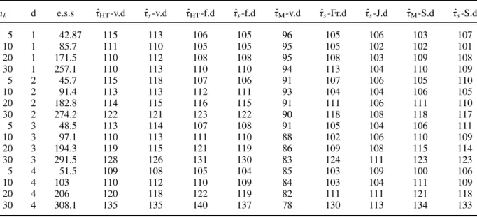
Table 2. Simulation of efficiencies in the synthetic zirconium distribution population in a region on the moon. nh d e.s.s τˆHT-v.d τˆs-v.d τˆHT-f.d τˆs-f.d τˆM-v.d τˆs-Fr.d τˆs-J.d τˆM-S.d τˆs-S.d 5 1 42.87 115 113 106 105 96 105 106 103 107 10 1 85.7 111 110 105 105 95 105 102 102 101 20 1 171.5 110 112 108 108 95 108 103 109 108 30 1 257.1 110 113 110 110 94 113 104 110 109 5 2 45.7 115 118 107 106 91 107 106 105 110 10 2 91.4 113 113 112 111 93 104 104 106 105 20 2 182.8 114 115 116 115 91 111 106 111 110 30 2 274.2 122 121 123 122 90 118 108 118 117 5 3 48.5 113 114 107 108 91 105 104 106 111 10 3 97.1 110 113 111 110 88 102 106 110 109 20 3 194.3 119 115 121 119 86 109 108 115 114 30 3 291.5 128 126 131 130 83 124 111 123 123 5 4 51.5 109 108 105 104 85 103 109 100 106 10 4 103 110 112 110 109 84 103 104 111 109 20 4 206 120 118 122 119 82 111 111 121 118 30 4 308.1 135 135 140 137 78 130 113 134 133 The population is partitioned into eight strata and the conditionCisyhi≥1. The estimatorsτˆHT,τˆs, andτˆMare, respectively, the HT type

estimator, sample mean type estimator and Murthy’s estimator. The notations e.s.s, v.d, f.d, Fr.d, J.d and S.d are, respectively, the effective sample size, variable sample size design, fixed sample size design, Francis’s design, Jolly–Hompton’s design and Salehi–Smith’s design.

Table 3. Simulation of relative biases in HPK.

nh d e.s.s τˆHT-v.d τˆs-v.d τˆHT-f.d τˆs-f.d τˆs-Fr.d τˆs-J.d τˆs-S.d 5 1 20.6 −0.02 −0.02 −0.009 −0.015 −0.013 −0.015 −0.022 10 1 41.1 −0.01 −0.01 −0.008 −0.009 −0.006 −0.004 −0.008 50 1 205.6 −0.001 −0.003 −0.001 −0.001 −0.002 −0.0007 −0.0012 100 1 411 −0.0005 −0.0008 −0.0009 −0.001 −0.0004 −0.0003 −0.0005 200 1 822 −0.00004 −0.00007 −0.0003 −0.00002 −0.0002 −0.0002 −0.0005 5 2 21.1 −0.04 −0.04 −0.017 −0.017 −0.013 −0.018 −0.032 10 2 42.2 −0.02 −0.02 −0.014 −0.013 −0.008 −0.005 −0.018 50 2 211.1 −0.01 −0.01 −0.002 −0.002 −0.005 −0.0016 −0.0017 100 2 422.3 −0.001 −0.002 −0.001 −0.001 −0.001 −0.0008 −0.0003 200 2 844.6 −0.001 −0.001 −0.0003 −0.0009 −0.00002 −0.00003 −0.0002 5 3 21.7 −0.04 −0.04 −0.025 −0.03 −0.029 −0.02 −0.047 10 3 43.34 −0.03 −0.03 −0.017 −0.016 −0.014 −0.008 −0.022 50 3 216.8 −0.01 −0.01 −0.002 −0.003 −0.004 −0.0017 −0.002 100 3 433.5 −0.0006 −0.003 −0.001 −0.002 −0.002 −0.0003 −0.0005 200 3 866.9 −0.001 −0.001 −0.0003 −0.0005 −0.0005 −0.00006 −0.0002 5 4 22.2 −0.06 −0.06 −0.032 −0.029 −0.028 −0.019 −0.052 10 4 44.5 −0.03 −0.03 −0.018 −0.016 −0.02 −0.009 −0.029 50 4 222.3 −0.01 −0.01 −0.002 −0.003 −0.003 −0.003 −0.0022 100 4 444.5 −0.003 −0.004 −0.001 −0.002 −0.002 −0.002 −0.0007 200 4 889.2 −0.001 −0.002 −0.0005 −0.0005 −0.001 −0.00003 −0.0002 The population is partitioned into four strata and the conditionCisyhi>20. The estimatorsτˆHTandτˆsare, respectively, the HT type

estimator and sample mean type estimator. The notations e.s.s, v.d, f.d, Fr.d, J.d and S.d are, respectively, the effective sample size, variable sample size design, fixed sample size design, Francis’s design, Jolly–Hampton’s design and Salehi–Smith’s design.

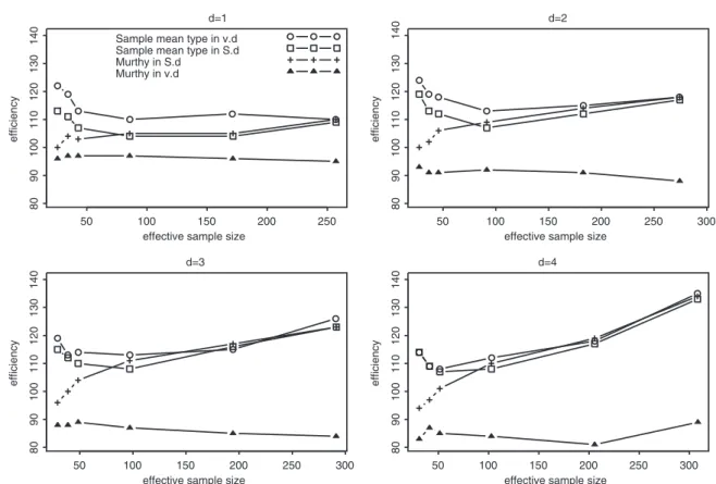
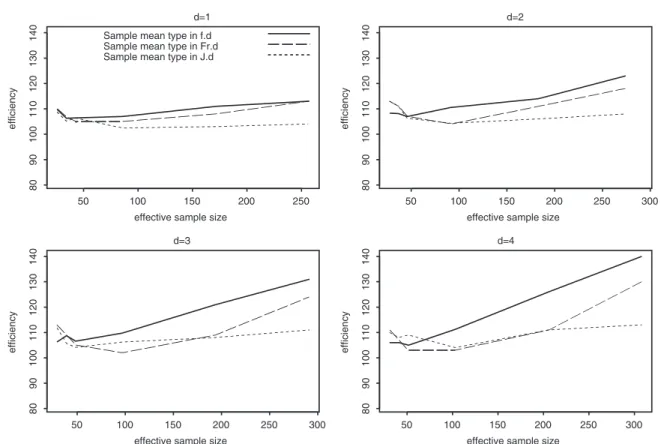
the variable and fixed designs are approximately identical. To make clearer the plots in Figures 3– 8 we only draw the sample mean type for the variable sample size design and fixed sample size design. Figures 3 and 6 show that the sample mean type for the variable sample size design is more efficient than other estimators in variable designs. For Salehi–Smith’s design, whennh1 is small (for HPKnh1 <20 and for SZMnh1 <10) the sample mean type is more efficient than Murthy’s estimator, but whennh1 is large, the estimators are approximately identical. In Figure 4, we can see the sample mean type for the fixed sample size design and Francis’s design has approximately

601 602 603 604 605 606 607 608 609 610 611 612 613 614 615 616 617 618 619 620 621 622 623 624 625 626 627 628 629 630 631 632 633 634 635 636 637 638 639 640 641 642 643 644 645 646 647 648 649 650

Figure 3. Efficiency of the sample mean type and Murthy’s estimators in the variable sample size designs in the HPK population. The first phase sample size in each stratum is represented respectively as the set {5,6, . . . ,10,20, . . . ,50,100,200}.

Figure 4. Efficiency of the sample mean type estimator in the fixed sample size designs in the HPK population. The first phase sample size in each stratum is represented respectively as the set{5,6, . . . ,10,20, . . . ,50,100,200}.

651 652 653 654 655 656 657 658 659 660 661 662 663 664 665 666 667 668 669 670 671 672 673 674 675 676 677 678 679 680 681 682 683 684 685 686 687 688 689 690 691 692 693 694 695 696 697 698 699 700

Figure 5. Efficiency of the best estimators in all designs in the HPK population. The first phase sample size in each stratum is represented respectively as the set{5,7. . . ,10,20, . . . ,50,100,200}.

Figure 6. Efficiency of the sample mean type and Murthy’s estimators in the variable sample size designs in the SZM population. The first phase sample size in each stratum is represented respectively as the set{3,4,5,10,30}.

701 702 703 704 705 706 707 708 709 710 711 712 713 714 715 716 717 718 719 720 721 722 723 724 725 726 727 728 729 730 731 732 733 734 735 736 737 738 739 740 741 742 743 744 745 746 747 748 749 750

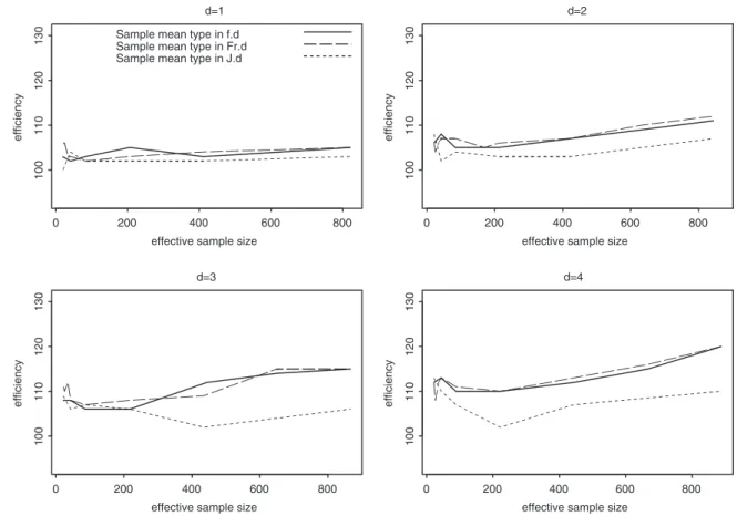
Figure 7. Efficiency of the sample mean type estimator in the fixed sample size designs in the SZM population. The first phase sample size in each stratum is represented respectively as the set{3,4,5,10,20,30}.

Figure 8. Efficiency of the best estimators in all designs in the SZM population. The first phase sample size in each stratum is represented respectively as the set{3,4,5,10,20,30}.

751 752 753 754 755 756 757 758 759 760 761 762 763 764 765 766 767 768 769 770 771 772 773 774 775 776 777 778 779 780 781 782 783 784 785 786 787 788 789 790 791 792 793 794 795 796 797 798 799 800

identical efficiencies. They are also more efficient than estimator of Jolly–Hampton’s design. In Figure 7, the sample mean type estimator for the fixed sample size design is more efficient than others.

For both the fixed and variable sample size designs, since the sample mean type estimator for the fixed and variable sample sizes were more efficient than estimators of introduced designs, we plot them in Figures 5 and 8. The variable sample size design was generally more efficient than the fixed sample size design at smaller effective sample sizes and the fixed sample size design was more efficient at larger effective sample sizes. Comparing the variable and fixed sample size designs, the results displayed in tables suggest that up until the first phase the allocation is about 1/4 of the size of the population, and the variable size design is the more efficient of the two. When the first phase allocation is approximately more than 1/4 of the size of the population, the fixed size design is more efficient.

It turns out that Murthy’s estimator (τˆM), which is derived from Rao-Blackwell procedure, is not an efficient estimator in our study. Results of Brownet al.[6] showed that this estimator can be efficient for very rare population. However, the weight pˆh in τˆM depends on the first phase sample only, which can be a justification for not being an efficient sampling, especially when the first phase sample size is a small proportion of the final sample size.

In Table 3, for each estimator the relative bias in the fixed sample size design is smaller than the relative bias of that estimator in the variable sample size design. Relative bias will increase as multiplierdincreases or the first phase sample sizenh1in each stratum is small, for all estimators. Ford < 5 andnh1 >2 the bias was negligible.

Acknowledgements

We thank Dr K.H. Low for providing us the moon data and its figure. Dr Salehi and Moradi’s works were partially supported by the CEAMA of Isfahan University of Technology.

References

[1] W.G. Cochran,Sampling Techniques, 3rd ed., Wiley, New York, 1977.

Q5

[2] S.K. Thompson and G.A.F. Seber,Adaptive sampling, Wiley, New York, 1996.

[3] R.I.C.C. Francis,An adaptive strategy for stratified random trawl survey, N. Z. J. Mar. Freshwater Res. 18 (1984), pp. 59–71.

[4] G.M. Jolly and I. Hampton, A stratified random transect design for acoustic surveys of fish stochs, Can. J. Fish. Aquat. Sci. 47 (1990), pp. 1282–1291.

[5] M.M. Salehi and D.R. Smith,Two-stage sequential sampling, J. Agric. Biol. Environ. Stat. 10(1) (2005), pp. 84–103. [6] J.A. Brown, M.M. Salehi, M. Moradi, G. Bell, and D. Smith,Adaptive two-stage sequential sampling, Popul. Ecol.

50 (2008), pp. 239–245.

[7] D.G. Horvitz and D.J. Thompson,A generalization of sampling without replacement a finite universe, J. Am. Statist.

Q6

Assoc. 47 (1952), pp. 663–685.

[8] M.C. Christman,Adaptive two-stage one-per-stratum sampling, Environ. Ecol. Stat. 10 (2003), pp. 43–60. [9] M. Moradi, M.M. Salehi, and P.S. Levy,Using general inverse sampling design to avoid undefined estimator, J.

Probab. Statist. Sci. 5(2) (2007), pp. 137–150.

[10] K.H. Low, G. Gordon, J. Dolan, and P. Khosla, Adaptive sampling for multi-robot wide-area exploration, in Proceedings of the IEEE International Conference on Robotics and Automation (ICRA’07), 2007, pp. 755–760. [11] C.E. Särndal, B. Swensson, and J. Wretman,Model Assisted Survey Sampling, Springer Verlag, New York, 1992.

Q7

Appendix

In order to show that the bias ofτˆsis negative, we prove the expectation of the ratio of units satisfying the conditionCin the sample is smaller than the ratio in the population. The ratio in the population and sample are, respectively,k/Nand (l1+l2)/(n1+dl1), the subscripthis eliminated for simplicity.

801 802 803 804 805 806 807 808 809 810 811 812 813 814 815 816 817 818 819 820 821 822 823 824 825 826 827 828 829 830 831 832 833 834 835 836 837 838 839 840 841 842 843 844 845 846 847 848 849 850

We first show that the functionf (l1)=(l1+E2(l2))/(n1+dl1)is a convex function whereE2(.)is the expectation, given the first phase sample.

f (l1)= l1+E2(l2) n1+dl1 = l1+dl1K−l1/(N−n1) n1+dl1 = 1 N−n1 (N−n1+dK)l1−dl12 n1+dl1 4(f (l1))=f (l1+1)−f (l1)= 1 N−n1 (N−n1+dK)(l1+1)−d(l1+1)2 n1+d(l1+1) − 1 N−n1 (N−n1+dK)l1−dl₁2 n1+dl1 = 1 N−n1 −d2_l2 1−(2dn−d2)l1−dn+(N−n1+dK)n (n1+dl1)(n1+d(l1+1)) 42_{(f (l} 1))= 4(l1+1)− 4(l1) = 1 N−n1 −d2_(l 1+1)2−(2dn−d2)(l1+1)−dn+(N−n1+dK)n (n1+d(l1+1))(n1+d(l1+2)) − 1 N−n1 −d2_l2 1 −(2dn−d2)l1−dn+(N−n1+dK)n (n1+dl1)(n1+d(l1+1)) = 1 N−n1 −2dn(N+dK) (n1+dl1)(n1+d(l1+1))(n1+d(l1+2)) <0 Using the Jenssen inequality, we have

E µ _l 1+l2 n1+dl1 ¶ =E1 µ E2 µ _l 1+l2 n1+dl1 |l1 ¶¶ =E1 µ_l 1+E2(l2) n1+dl1 ¶ ≤ E(l1+l2) E(n1+dl1) = n1K/N (1+d(K−n1K/N )/(N−n1)) n1+dn1K/N = K N µ₁₊ dK/N 1+dK/N ¶ = K N.