MNP: R Package for Fitting the Multinomial Probit Model

(1)

May 2005, Volume 14, Issue 3. http://www.jstatsoft.org/

MNP

:

R

Package for Fitting the Multinomial Probit

Model

Kosuke Imai

Princeton University

David A. van Dyk University of California, Irvine

Abstract

MNPis a publicly availableRpackage that fits the Bayesian multinomial probit model via Markov chain Monte Carlo. The multinomial probit model is often used to analyze the discrete choices made by individuals recorded in survey data. Examples where the multi-nomial probit model may be useful include the analysis of product choice by consumers in market research and the analysis of candidate or party choice by voters in electoral studies. TheMNP software can also fit the model with different choice sets for each in-dividual, and complete or partial individual choice orderings of the available alternatives from the choice set. The estimation is based on the efficient marginal data augmentation algorithm that is developed by Imai and van Dyk(2005).

Keywords: data augmentation, discrete choice models, Markov chain Monte Carlo, preference data.

1. Introduction

This paper illustrates how to use MNP, a publicly available R (R Development Core Team 2005) package, in order to fit the Bayesian multinomial probit model via Markov chain Monte Carlo. The multinomial probit model is often used to analyze the discrete choices made by individuals recorded in survey data. Examples where the multinomial probit model may be useful include the analysis of product choice by consumers in market research and the analysis of candidate or party choice by voters in electoral studies. The MNPsoftware can also fit the model with different choice sets for each individual, and complete or partial individual choice orderings of the available alternatives from the choice set. We use Markov chain Monte Carlo (MCMC) for estimation and computation. In particular, we use the efficient marginal data augmentation MCMC algorithm that is developed by Imai and van Dyk(2005).

MNPcan be installed in the same way as otherRpackages via theinstall.packages("MNP")

(2)

Mac OS X, and Linux/UNIX platforms. Only three commands are necessary to use theMNP software;mnp()fits the multinomial probit model,summary()summarizes the MCMC output, andpredict()gives posterior prediction based on the fitted model. To run an example script, startRand run the following commands:

library(MNP) # loads the MNP package

example(mnp) # runs the example script

Details of the example script are given in Sections 3 and 4. Three appendices describe installation, the commands, and version history. We begin in Section2with a brief description of the multinomial probit model thatMNPis designed to fit.

2. The method

MNP implements the marginal data augmentation algorithms for posterior sampling in the multinomial probit model. The MCMC algorithm we implement here is fully described in Imai and van Dyk(2005); we use Scheme 1 of their Algorithm 1.

2.1. The multinomial probit model

Suppose we have a dataset of size n with p > 2 choices and k covariates. Here, choices refer to the number of classes in the multinomial model. The word “choices” is used because the model is often used to describe how individuals choose among a number of alternatives, e.g., how a voter chooses which candidate to vote for among four candidates running for a particular office. We focus on the case when p > 2 because when p = 2, the model reduces to the standard binomial probit model, which can be fit via the glm(, family =

binomial(probit))command in R. The multinomial probit model differs from the ordinal

probit model in that the former does not assume any inherent ordering on the choices. Thus, although the individuals may have preferences among the available alternatives these ordering are individual specific rather than being characteristics of the alternatives themselves. The ordinal probit model can be fitted via an MCMC algorithm inRby installing a package called MCMCpack(Martin and Quinn 2004).

Under the multinomial probit model, we assume a multivariate normal distribution on the latent variables,Wi = (Wi1, . . . , Wi,p−1).

Wi=Xiβ+ei, ei ∼N(0,Σ), fori= 1, . . . , n, (1) where Xi is a (p−1)×k matrix of covariates, β is k×1 vector of fixed coefficients, ei is (p−1)×1 vector of disturbances, and Σ is a (p−1)×(p−1) positive definite matrix. For the model to be identified, the first diagonal element of Σ is constrained, σ11= 1. The response

variable, Yi, is the index of the choice of individualiamong the alternatives in the choice set and is modeled in terms of this latent variable,Wi, via

Yi(Wi) =

0 if max(Wi)<0

j if max(Wi) =Wij >0 , fori= 1, . . . , n, andj= 1, . . . , p

−1, (2) whereYi equal to 0 corresponds to a base category.

(3)

The matrix Xi may include both specific and individual-specific variables. A choice-specific variable is a variable that has a value for each of the p choices, and these p values may be different for each individual (e.g., the price of a product in a particular region where an individual lives). Choice-specific variables are recorded relative to the baseline choice and thus there are p−1 recorded values for each individual. In this way a choice-specific variable is tabulated as a column in Xi. Individual-specific variables, on the other hand, take on a value for each individual, but are constant across the choices, e.g., the age or gender of the individual. These variables are tabulated via their interaction with each of the choice indicator variables. Thus, an individual-specific variable corresponds to p−1 columns ofXi and p−1 components ofβ.

2.2. The multinomial probit model with ordered preferences

In some cases, we observe a complete or partial ordering of p alternatives. For example, we may observe the preferences of each individual among different brands of a product. We denote the outcome variable in such situations by Y_i = {Y_i₁, . . . ,Y_ip} where i = 1, . . . , n

indexes individuals and j = 1, . . . , p represent alternatives. IfYij >Yij0 for somej 6=j0, we

say j is preferred to j0. IfY_ij =Y_ij0 for somej 6=j0, we say individual iis indifferent to the

choice between alternatives j andj0, but treat the data as if the actual ordering is unknown. In other words, formally we insist on strict inequalities among the preferences, but allow for some inequalities to be unobserved. The preference ordering is assumed to satisfy the usual axioms of preference comparability. Namely, preference is connected: For anyjand j0, either

Yij ≤ Yij0 orY_ij ≥ Y_ij0. Preference also must be transitive: for any j,j0, and j00, Y_ij ≤ Y_ij0

and Y_ij0 ≤ Y_ij00 implyY_ij ≤ Y_ij00. For notational simplicity and without loss of generality, we

assume that Y_ij takes an integer value ranging from 0 to p−1. We emphasize that we have not changed the model from Section 2.1. Rather, we simply have more observed data: the index of the choice of the individuali, Yi, can be computed from Yi. Thus, we continue to model the preference ordering, Y_i, in terms of a latent (multivariate normal) random vector,

Wi = (Wij, . . . , Wi,p−1), via

Y_ij(Wi) = #{Wij0 :W_ij0 < W_ij} for i= 1, . . . , n, and j= 1, . . . , p, (3)

where Wip = 0, the distribution of Wi is specified in equation 1, and #{· · · } indicates the number of elements in a finite set. This model can be fitted via a slightly modified version of the MCMC algorithm in Imai and van Dyk (2005). In particular, we need only modify the way in which Wij is sampled and use a truncation rule based on Equation 3.

2.3. Prior specification

Our prior distribution for the multinomial probit model is

β∼N(0, A−1) and p(Σ)∝ |Σ|−(ν+p)/2

trace(SΣ−1)−ν(p−1)/2

, (4)

whereA is the prior precision matrix ofβ,ν is the prior degrees of freedom parameter for Σ, and the (p−1)×(p−1) positive definite matrix S is the prior scale for Σ; we assume the first diagonal element ofS is one. The prior distribution on Σ is proper ifν ≥p−1, the prior mean of Σ is approximately equal toS ifν > p−2, and the prior variance of Σ increase asν

(4)

decreases as long as this variance exists. We also allow for an improper prior on β, which is

p(β)∝1 (i.e., A= 0).1

Alternate prior specifications were introduced by McCulloch and Rossi (1994) and McCul-loch, Polson, and Rossi(2000). The relative advantage of the various prior distributions are discussed byMcCullochet al.(2000),Nobile(2000), andImai and van Dyk(2005). We prefer our choice because it allows us to directly specify the prior distribution on the identifiable model parameters, allows us to specify an improper prior distribution on regression coefficient, and results in a Monte Carlo sampler that is relatively quick to converge. An implementation of of the sampler proposed byMcCulloch and Rossi(1994) has recently been released in the Rpackagebayesm (Rossi and McCulloch 2005).

2.4. Prediction under the multinomial probit model

Predictions of individual preferences given particular values of the covariates can be useful in interpreting the fitted model. Consider a value of the (p−1)×k matrix of covariates, X?, that may or may not correspond to the values for one of the observed individuals. We are interested in the distribution of the preferences among the alternatives in the choice set given this value of the covariates. Let Y? be the preferred choice and Y? _{= (}_Y?

1, . . . ,Yp?) indicate the ordering of the preferences among the available alternatives. As an example, one might be interested in Pr(Y? =j|X?) for somej. By varyingX?, one could explore how preferences are expected to change with covariates. Similarly, one might be interested in how relative preferences such as Pr(Y?

j >Yj?0 |X?) are expected to change with the covariates.

In the context of a Bayesian analysis, such predictive probabilities are computed via the posterior predictive distribution. This distribution conditions on the observed data, Y = (Y1, . . . , Yn) orY = (Y1, . . . ,Yn), but averages over the uncertainty in the model parameters. For example,

Pr(Y? =j|X?, Y) = Z

Pr(Y?=j|X?, β,Σ, Y)p(β,Σ|Y)d(β,Σ). (5) Thus, the posterior predictive distribution accounts for both variability in the response vari-able given the model parameters (i.e., the likelihood or sampling distribution) and the un-certainty in the model parameters as quantified in the posterior distribution. Monte Carlo evaluation of the posterior predictive distribution is easy once we obtain a Monte Carlo sam-ple of the model parameters from the posterior distribution: We simply samsam-ple according to the likelihood for each Monte Carlo sample from the posterior distribution. This involves sampling the latent variable under the model in (1) and computing the preferred choice using (2) or the ordering of preferences using (3).

3. Example 1: Detergent brand choice

In this and the next section, we describe the details of two examples ofMNP. In this section we use a market research dataset to illustrate the fitting of the multinomial probit model. In Section4we fit the multinomial probit model with ordered preference to a Japanese election

1_{Algorithm 2 of}_{Imai and van Dyk}₍₂₀₀₅_{) allows for a non zero prior mean for}_β_{. Because the update for}

Σ in this sampler is not exactly its complete conditional distribution, however, this algorithm may exhibit undesirable convergence properties in some situations.

(5)

dataset. We also describe how to perform convergence diagnostics of the MCMC sampler and analysis of the Monte Carlo output ofMNPusing an existingRpackage. Additional examples of MNPcan be found inImai and van Dyk(2005).

3.1. Preliminaries

Our first example analyzes a typical dataset in market research. The dataset contains infor-mation about the brand and price of the laundry detergent purchased by 2657 households originally analyzed by Chintagunta and Prasad (1998). The dataset contains the log prices of six detergent brands – Tide, Wisk, EraPlus, Surf, Solo, and All – as well as the brand chosen by each household (see AppendixCfor details about the dataset). We are interested in estimating the correlation between price and consumer choice.

We fit the multinomial probit model by using choice as the outcome variable and the other six variables as choice-specific covariates. After loading the MNP package, this can be ac-complished using the following three commands,

data(detergent)

res <- mnp(choice ~ 1, choiceX = list(Surf=SurfPrice, Tide=TidePrice, Wisk=WiskPrice, EraPlus=EraPlusPrice, Solo=SoloPrice, All=AllPrice),

cXnames = c("price"), data = detergent, n.draws = 10000, burnin = 2000, thin = 3, verbose = TRUE)

summary(res)

The first command loads the example dataset and stores it as the data frame calleddetergent. The second command fits the multinomial probit model. The default base category in this case isAll. (The default base category inMNPis the first factor level of the outcome variable,Y.) Each household chooses among the six brands of laundry detergent, i.e., p = 6. We specify the choice-specific variables,choiceX, using a named list. The elements of the list are the log price of each detergent brand and they are named after the levels of factor variable,choice. We also name the coefficient for this set of choice-specific variables by using cXnames. The argument data allows us to specify the name of the data frame where the data are stored. The model estimates five intercepts and the price coefficient as well as 14 parameters in the covariance matrix, Σ.

We use the default prior distribution; an improper prior distribution forβ and a diffuse prior distribution for Σ withν=p= 6 andS =I. We sample 10,000 replications of the parameter from the resulting posterior distribution, saving every fourth sample after discarding the first 2,000 samples as specified by the arguments, n.draws, thin, and burnin. The argument

verbose = TRUEspecifies that a progress report and other useful messages be printed while the MCMC sampler is running. Thesummary(res)command gives a summary of the output including the posterior means and standard deviations of the parameters. The summary is based on the single MCMC chain produced with this call ofMNP. Before we can reliably draw conclusions based on these results, we must be sure the chain has converged. Convergence diagnostics are discussed and illustrated in Section3.2. The result of the call ofsummary(res)

(6)

Call:

mnp(formula = choice ~ 1, data = detergent, choiceX = list(Surf = SurfPrice, Tide = TidePrice, Wisk = WiskPrice, EraPlus = EraPlusPrice,

Solo = SoloPrice, All = AllPrice), cXnames = c("price"), n.draws = 10000, burnin = 2000, thin = 3, verbose = TRUE)

Coefficients: mean std.dev. 2.5% 97.5% (Intercept):EraPlus 2.567 0.238 2.123 3.03 (Intercept):Solo 1.722 0.247 1.248 2.25 (Intercept):Surf 1.572 0.163 1.259 1.91 (Intercept):Tide 2.716 0.252 2.269 3.22 (Intercept):Wisk 1.620 0.162 1.328 1.96 price -82.102 8.952 -99.896 -66.32 Covariances: mean std.dev. 2.5% 97.5% EraPlus:EraPlus 1.00000 0.00000 1.00000 1.00 EraPlus:Solo 0.82513 0.26942 0.31029 1.36 EraPlus:Surf 0.17021 0.16115 -0.15810 0.48 EraPlus:Tide 0.24872 0.12956 0.00253 0.52 EraPlus:Wisk 0.88170 0.16614 0.54500 1.20 Solo:Solo 2.56481 0.68678 1.53276 4.25 Solo:Surf 0.45246 0.34572 -0.28018 1.13 Solo:Tide 0.50836 0.32706 -0.09069 1.22 Solo:Wisk 1.46997 0.44596 0.65506 2.45 Surf:Surf 1.69005 0.50978 0.92334 2.82 Surf:Tide 0.80762 0.30381 0.34019 1.44 Surf:Wisk 1.01614 0.36503 0.44121 1.85 Tide:Tide 1.32024 0.41669 0.62898 2.25 Tide:Wisk 1.05396 0.30137 0.59323 1.74 Wisk:Wisk 2.58761 0.55076 1.68773 3.82

Base category: All

Number of alternatives: 6 Number of observations: 2657 Number of stored MCMC draws: 2000

We emphasize that these results are preliminary because convergence has not yet been as-sessed. Thus, we delay interpretation of the fit until Section3.3, after we discuss convergence diagnostics in Section3.2.

3.2. Using coda for convergence diagnostics and output analysis

It is possible to use coda (Plummer, Best, Cowles, and Vines 2005), to perform various convergence diagnostics, as well as to summarize results. Thecodapackage requires a matrix

(7)

of posterior draws for relevant parameters to be saved as anmcmc object. Here, we illustrate how to usecodato calculate the Gelman-Rubin convergence diagnostic statistic (Gelman and Rubin 1992). This diagnostic is based on multiple independent Markov chains initiated at over-dispersed starting values. Here, we obtain these chains by independently running the

mnp()command three times, specifying different starting values for each time. This can be accomplished by typing the following commands at theRprompt,

data(detergent)

res1 <- mnp(choice ~ 1, choiceX = list(Surf=SurfPrice, Tide=TidePrice,

Wisk=WiskPrice, EraPlus=EraPlusPrice, Solo=SoloPrice, All=AllPrice),

cXnames = c("price"), data = detergent, n.draws = 50000, verbose = TRUE)

coef.start = c(1, -1, 1, -1, 1, -1)*10,

cov.start = matrix(0.5, ncol=5, nrow=5) + diag(0.5, 5), cXnames = c("price"), data = detergent, n.draws = 50000, verbose = TRUE)

coef.start=c(-1, 1, -1, 1, -1, 1)*10,

cov.start = matrix(0.9, ncol=5, nrow=5) + diag(0.1, 5), cXnames = c("price"), data = detergent, n.draws = 50000, verbose = TRUE)

where we save the output of each chain separately asres1,res2, andres3. The first chain is initiated at the default starting values for all parameters; i.e., a vector of zeros forβ and an identity matrix for Σ. The second chain is run starting from a vector of three 10’s and three

−10’s for β and a matrix with all diagonal elements equal to 1 and all correlations equal to 0.5 for Σ. Finally, the third chain is run starting from a permutation of the starting value used for β in the second chain, and a matrix with all diagonal elements equal to 1 and all correlations equal to 0.9 for Σ. We again use the default prior specification and obtain 50,000 draws for each chain.

We store the output from each of the three chains as an object of classmcmc, and then combine them into a single list using the following commands,

library(coda)

res.coda <- mcmc.list(chain1=mcmc(res1$param[,-7]), chain2=mcmc(res2$param[,-7]), chain3=mcmc(res3$param[,-7]))

where the first command loads thecoda package2 and the second command saves the results

(8)

in-as an object of clin-assmcmc.list, which is calledres.coda. We exclude the 7th column of each chain, because this column corresponds to the first diagonal element of the covariance matrix which is always equal to 1. The following command computes the Gelman-Rubin statistic from these three chains,

gelman.diag(res.coda, transform = TRUE)

where transform = TRUE applies log or logit transformation as appropriate to improve the normality of each of the marginal distributions. Gelman, Carlin, Stern, and Rubin (2004) suggest computing the statistic for each scalar estimate of interest, and to continue to run the chains until the statistics are all less than 1.1. Inference is then based on the Monte Carlo sample obtained by combining the second half of each of the chains. The output of the codacommand lists the value and a 97.5% upper limit of the Gelman-Rubin statistic for each parameter.

Potential scale reduction factors:

Point est. 97.5% quantile

(Intercept):EraPlus 1.01 1.02 (Intercept):Solo 1.03 1.08 (Intercept):Surf 1.01 1.05 (Intercept):Tide 1.01 1.02 (Intercept):Wisk 1.01 1.04 price 1.01 1.02 EraPlus:Solo 1.02 1.03 EraPlus:Surf 1.02 1.04 EraPlus:Tide 1.03 1.08 EraPlus:Wisk 1.04 1.13 Solo:Solo 1.01 1.04 Solo:Surf 1.01 1.02 Solo:Tide 1.02 1.07 Solo:Wisk 1.00 1.00 Surf:Surf 1.00 1.00 Surf:Tide 1.01 1.04 Surf:Wisk 1.02 1.06 Tide:Tide 1.02 1.06 Tide:Wisk 1.02 1.08 Wisk:Wisk 1.01 1.04 Multivariate psrf 1.07+0i

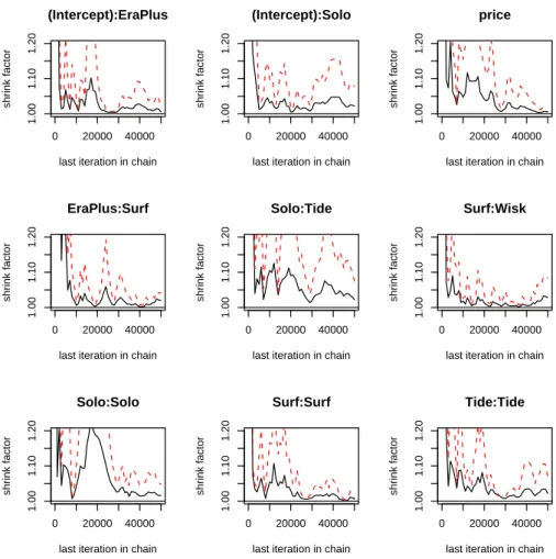
The Gelman-Rubin statistics are all less than 1.1, suggesting satisfactory convergence has been achieved. (Note that the 97.5conservative user might want to obtain a set of longer Markov chains and recompute the Gelman-Rubin statistics.) It may also be useful to examine the

(9)

0 20000 40000

1.00

1.10

1.20

last iteration in chain

shrink factor (Intercept):EraPlus 0 20000 40000 1.00 1.10 1.20

shrink factor (Intercept):Solo 0 20000 40000 1.00 1.10 1.20

shrink factor price 0 20000 40000 1.00 1.10 1.20

shrink factor EraPlus:Surf 0 20000 40000 1.00 1.10 1.20

shrink factor Solo:Tide 0 20000 40000 1.00 1.10 1.20

shrink factor Surf:Wisk 0 20000 40000 1.00 1.10 1.20

shrink factor Solo:Solo 0 20000 40000 1.00 1.10 1.20

shrink factor Surf:Surf 0 20000 40000 1.00 1.10 1.20

shrink factor

Tide:Tide

Figure 1: The Gelman-Rubin Statistic Computed with Three Independent Markov Chains for Selected Parameters in the Detergent Example. The first row represents three coefficients, the second row represents three covariances, and the third row represents three variance parameters.

change in the value of the Gelman-Rubin statistic over the iterations. The following commands produce a graphical summary of the progression of the statistics over iterations.

gelman.plot(res.coda, transform = TRUE, ylim = c(1,1.2))

whereylim = c(1,1.2)specifies the range of the vertical axis of the plot. The results appear in Figure1, as a cumulative evaluation of the Gelman-Rubin statistic over iterations for nine selected parameters. (Three coefficients appear in the first row; three covariance parameters appear in the second row; and three variance parameters appear in the third row.)

Thecodapackage can also be used to produce univariate time-series plots of the three chains and univariate density estimate of the posterior distribution. The following commands create these graphs for the price coefficient.

(10)

25000 30000 35000 40000 45000 50000 −110 −90 −70 Iterations −110 −90 −80 −70 −60 −50 0.00 0.01 0.02 0.03 0.04 N = 75000 Bandwidth = 0.9464

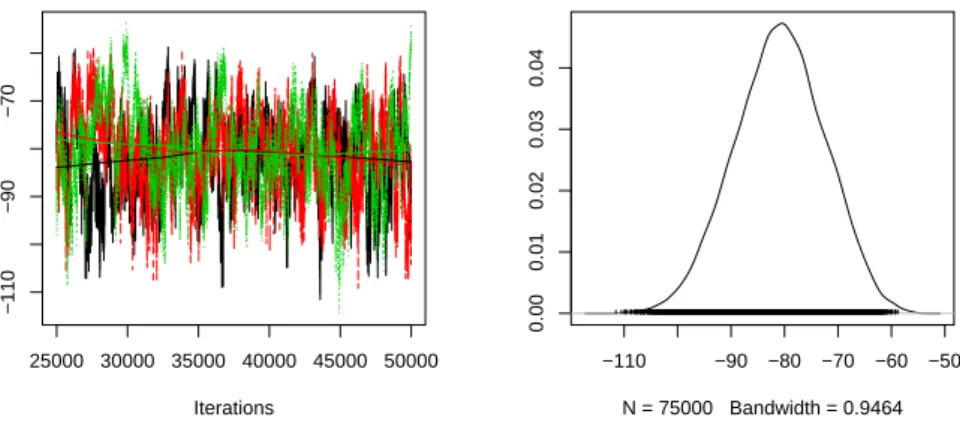
Figure 2: Time-series Plot of Three Independent Markov Chains (Left Panel) and A Density Estimate of the Posterior Distribution of the Price Coefficient (Right Panel). The time-series plot overlays the three chains, each in a different color. A lowess smoothed line is also plotted for each of the three chains. The density estimate is based on all three chains.

res.coda <- mcmc.list(chain1=mcmc(res1$param[25001:50000, "price"], start=25001), chain2=mcmc(res2$param[25001:50000, "price"], start=25001), chain3=mcmc(res3$param[25001:50000, "price"], start=25001)) plot(res.coda, ylab = "price coefficient")

Figure2presents the resulting plots. The left panel overlays the time-series plot for each chain with a different color representing each chain. The right panel shows the kernel-smoothed density estimate of the posterior distribution. One can also apply an array of other functions tores.coda. See thecodahomepage, , for details.

3.3. Final analysis and conclusions

In the final analysis, we combine the second half of each of the three chains. This is accom-plished using the following command that saves the last 25,000 draws from each chain as an

mcmcobject and combines the mcmc objects into a list,

res.coda <- mcmc.list(chain1=mcmc(res1$param[25001:50000,-7], start=25001), chain2=mcmc(res2$param[25001:50000,-7], start=25001), chain3=mcmc(res3$param[25001:50000,-7], start=25001)) summary(res.coda)

The second command produces the following summary of the posterior distribution for each parameter based on the combined Monte Carlo sample.

Iterations = 25001:50000 Thinning interval = 1 Number of chains = 3

(11)

1. Empirical mean and standard deviation for each variable, plus standard error of the mean:

Mean SD Naive SE Time-series SE

(Intercept):EraPlus 2.5398 0.2300 0.0008400 0.014332 (Intercept):Solo 1.7218 0.2227 0.0008131 0.012972 (Intercept):Surf 1.5634 0.1663 0.0006072 0.010462 (Intercept):Tide 2.6971 0.2374 0.0008670 0.015153 (Intercept):Wisk 1.6155 0.1594 0.0005822 0.010221 price -80.9097 8.4292 0.0307791 0.556483 EraPlus:Solo 0.8674 0.2954 0.0010787 0.021698 EraPlus:Surf 0.1226 0.1991 0.0007269 0.014043 EraPlus:Tide 0.2622 0.1525 0.0005568 0.009833 EraPlus:Wisk 0.9062 0.1912 0.0006982 0.012893 Solo:Solo 2.6179 0.7883 0.0028785 0.055837 Solo:Surf 0.5348 0.4307 0.0015728 0.030113 Solo:Tide 0.5570 0.3544 0.0012941 0.024548 Solo:Wisk 1.5442 0.4643 0.0016954 0.031574 Surf:Surf 1.6036 0.4758 0.0017374 0.031269 Surf:Tide 0.7689 0.2992 0.0010926 0.020253 Surf:Wisk 0.9949 0.3548 0.0012955 0.022963 Tide:Tide 1.2841 0.3660 0.0013364 0.024095 Tide:Wisk 1.0658 0.3147 0.0011492 0.020229 Wisk:Wisk 2.5801 0.5523 0.0020167 0.034974

2. Quantiles for each variable:

2.5% 25% 50% 75% 97.5% (Intercept):EraPlus 2.09105 2.38514 2.5321 2.6926 3.0022 (Intercept):Solo 1.28315 1.57316 1.7219 1.8705 2.1639 (Intercept):Surf 1.24132 1.45272 1.5583 1.6701 1.9023 (Intercept):Tide 2.23562 2.53443 2.6886 2.8544 3.1721 (Intercept):Wisk 1.31120 1.50841 1.6104 1.7191 1.9429 price -97.62406 -86.61736 -80.7783 -75.1013 -64.9720 EraPlus:Solo 0.32811 0.65755 0.8480 1.0694 1.4666 EraPlus:Surf -0.24159 -0.01596 0.1131 0.2507 0.5491 EraPlus:Tide -0.02109 0.16081 0.2571 0.3527 0.5957 EraPlus:Wisk 0.54089 0.77643 0.9035 1.0331 1.2917 Solo:Solo 1.37468 2.02720 2.5225 3.0985 4.4160 Solo:Surf -0.31143 0.25493 0.5251 0.8180 1.3880 Solo:Tide -0.05172 0.30518 0.5297 0.7740 1.3106 Solo:Wisk 0.74682 1.21192 1.5131 1.8380 2.5445 Surf:Surf 0.86883 1.25552 1.5377 1.8834 2.6935 Surf:Tide 0.30606 0.55218 0.7285 0.9413 1.4556 Surf:Wisk 0.40231 0.74907 0.9579 1.1957 1.8026 Tide:Tide 0.69841 1.02206 1.2396 1.4999 2.1100 Tide:Wisk 0.51732 0.84824 1.0411 1.2556 1.7579 Wisk:Wisk 1.60662 2.18760 2.5407 2.9238 3.7722

(12)

The output shows the mean, standard deviation, and various percentiles of the posterior distributions of the coefficients and the elements of the variance-covariance matrix. The base category is the detergentAll. Separate intercepts are estimated for each detergent. The price coefficient is negative and highly statistically significant, agreeing with the standard economic expectation that consumers are less likely to buy more expensive goods.

MNP also allows one to calculate the posterior predictive probabilities of each alternative being most preferred given a particular value of the covariates. For example, one can calculate the posterior predictive probabilities using the covariate values of the first two observations by using the predict() command,

predict(res1, newdata = detergent[1:2,],

newdraw = rbind(res1$param[25001:50000,], res2$param[25001:50000,],

res3$param[25001:50000,]), type = "prob")

whereres1is the output object from themnp()command, and we setnewdatato the first two observations of the detergent data set and newdraw to the combined draws from the second half of three chains. Setting type = "prob" causes the function predict() to return the posterior predictive probabilities. It is also possible to return a Monte Carlo sample of the the alternative that is most preferred (type = "choice"), a Monte Carlo sample of the latent variables (type = "latent"), or a Monte Carlo sample of the preference-ordered alternatives (type = "order"). (See AppendixBor typehelp(predict.mnp)inRfor more details about

the predict()function inMNP.) The above command yields the following output,

All EraPlus Solo Surf Tide Wisk

[1,] 0.01281333 0.1946400 0.12292 0.46208000 0.1401733 0.06737333 [2,] 0.04649333 0.1262133 0.05996 0.03169333 0.3589867 0.37665333

The result indicates that the posterior predictive probability of purchasing Surfis the largest for households with covariates equal to those in the first household in the data set. Under the model, approximately 46% of such households will purchase Surf. On the other hand,Allis the brand least likely to be purchased by these households. The households with covariates equal to the second household are most likely to buy Wisk. Also, they are almost equally likely to purchase Tide. (The posterior predictive probabilities of buying Wisk andTide are both around 0.35)

4. Example 2: Voters’ preference of political parties

Our second example illustrates how to fit the multinomial probit model with ordered prefer-ences (see Section 2.2).

4.1. Preliminaries

We analyze a survey dataset describing the preferences of individual voters in Japan among the political parties. Political scientists may be interested in using the gender, age and education level of voters to predict their party preferences (see AppendixCfor details about the dataset). The outcome variable is a vector of relative preferences for each of the four

(13)

parties, i.e., p = 4. Each of 418 voters is asked to give a score between 0 and 100 to each party. For example, the first voter in the dataset has the following preferences.

LDP NFP SKG JCP

80 75 80 0

That is, this voter prefers LDP and SKG to NFP and JCP, and between the latter two, she prefers NFPtoJCP. AlthoughLDPandSKGhave the same preference, we do not constrain the estimated preferences to be the same for these two alternatives. Under the Gaussian random utility model, the probability that the two alternatives having exactly the same preferences is zero. Therefore, inequality constraints are respected, but equality constraints are not. Furthermore, we only preserve the ranking, not the relative numerical values. Therefore, the following coding of the variables, for our purposes, is equivalent to that given above,

LDP NFP SKG JCP

3 2 3 1

Finally, it is possible to have non-response for one of the categories; e.g., no candidate from a particular party may run in a certain district. If NFP = NA, we have no information about the relative ranking of NFP.

LDP NFP SKG JCP

3 NA 3 1

In this case, there is no constraint when estimating the preference for this alternative; only the inequality constraint, (LDP, SKG) > JCP, is imposed.

All three covariates – gender, education, and age of voters – are individual-specific variables rather than choice-specific ones. The model estimates three intercepts and 9 coefficients along with 6 parameters in the covariance matrix. The following commands fit the model,

data(japan)

res <- mnp(cbind(LDP, NFP, SKG, JCP) ~ gender + education + age, data = japan, n.draws = 10000, verbose = TRUE)

summary(res)

The first command loads the dataset, and the second command fits the model. The base category isJCP, which is the last column of the outcome matrix. The default prior distribution is used as in the previous example: an improper prior distribution for β and a diffuse prior distribution for Σ with ν =p = 4 andS =I. 10,000 draws are obtained with no burnin or thinning. The final command summarizes the Monte Carlo sample and gives the following output,

(14)

Call:

mnp(formula = cbind(LDP, NFP, SKG, JCP) ~ gender + education + age, data = japan, n.draws = 10000, verbose = TRUE)

Coefficients: mean std.dev. 2.5% 97.5% (Intercept):LDP 0.615184 0.517157 -0.386151 1.61 (Intercept):NFP 0.689753 0.568109 -0.419521 1.79 (Intercept):SKG 0.133961 0.455960 -0.758883 1.02 gendermale:LDP 0.099748 0.152323 -0.194786 0.40 gendermale:NFP 0.216824 0.166103 -0.102108 0.54 gendermale:SKG 0.132661 0.134605 -0.127145 0.40 education:LDP -0.107038 0.074792 -0.253483 0.04 education:NFP -0.107222 0.082324 -0.270127 0.05 education:SKG -0.003728 0.066429 -0.132496 0.13 age:LDP 0.013518 0.006122 0.001492 0.03 age:NFP 0.006948 0.006783 -0.006572 0.02 age:SKG 0.009653 0.005431 -0.000812 0.02 Covariances: mean std.dev. 2.5% 97.5% LDP:LDP 1.0000 0.0000 1.0000 1.00 LDP:NFP 1.0502 0.0585 0.9373 1.16 LDP:SKG 0.7070 0.0622 0.5822 0.82 NFP:NFP 1.4068 0.1359 1.1682 1.70 NFP:SKG 0.7452 0.0864 0.5800 0.91 SKG:SKG 0.6913 0.0874 0.5296 0.87 Base category: JCP Number of alternatives: 4 Number of observations: 418

Number of stored MCMC draws: 10000

4.2. Convergence diagnostics, final analysis, and conclusions

In order to evaluate convergence of the MCMC sampler, we again obtain three independent Markov chains by running themnp()command three times with three sets of different starting values. We use starting values that are relatively dispersed given the preliminary analysis of the previous section. Note that when fitting the multinomial probit model with ordered preferences, the algorithm requires the starting values of the latent variable to respect the order constraints of equation (3). Therefore, the starting values of the parameters cannot be too far away from the posterior mode. The following commands fits the model with the default starting value and two sets of overdispersed starting values,

res1 <- mnp(cbind(LDP, NFP, SKG, JCP) ~ gender + education + age, data = japan, n.draws = 50000, verbose = TRUE)

(15)

res2 <- mnp(cbind(LDP, NFP, SKG, JCP) ~ gender + education + age, data = japan, coef.start = c(1, -1, 1, -1, 1, -1, 1, -1, 1, -1, 1, -1),

cov.start = matrix(0.5, ncol=3, nrow=3) + diag(0.5, 3), n.draws = 50000, verbose = TRUE)

res3 <- mnp(cbind(LDP, NFP, SKG, JCP) ~ gender + education + age, data = japan, coef.start = c(-1, 1, -1, 1, -1, 1, -1, 1, -1, 1, -1, 1),

cov.start = matrix(0.9, ncol=3, nrow=3) + diag(0.1, 3), n.draws = 50000, verbose = TRUE)

We follow the commands used in Section 3.2 and compute the Gelman-Rubin statistic for each parameter. Upon examination of the resulting statistics, we determined that satisfactory convergence has been achieved. For example, the value of the Gelman-Rubin statistic is less than 1.01 for all the parameters. Hence, we base our final analysis on the combined draws from the second half of the three chains (i.e., a total of 75,000 draws using 25,000 draws from each chain). Posterior summaries can be obtained using thecoda package as before,

Iterations = 25001:50000 Thinning interval = 1 Number of chains = 3

Sample size per chain = 25000

1. Empirical mean and standard deviation for each variable, plus standard error of the mean:

Mean SD Naive SE Time-series SE

(Intercept):LDP 0.60167 0.51421 1.88e-03 8.05e-03

(Intercept):NFP 0.68294 0.56867 2.08e-03 7.95e-03

(Intercept):SKG 0.12480 0.45680 1.67e-03 7.25e-03

gendermale:LDP 0.10668 0.15448 5.64e-04 2.95e-03

gendermale:NFP 0.22240 0.16983 6.20e-04 2.91e-03

gendermale:SKG 0.13897 0.13753 5.02e-04 2.70e-03

education:LDP -0.10517 0.07643 2.79e-04 1.35e-03

education:NFP -0.10634 0.08448 3.08e-04 1.28e-03

education:SKG -0.00258 0.06766 2.47e-04 1.18e-03

age:LDP 0.01361 0.00617 2.25e-05 9.90e-05

age:NFP 0.00698 0.00680 2.48e-05 1.01e-04

age:SKG 0.00972 0.00547 2.00e-05 9.13e-05

LDP:NFP 1.05535 0.05508 2.01e-04 1.15e-03

LDP:SKG 0.71199 0.06125 2.24e-04 1.59e-03

NFP:NFP 1.41860 0.13540 4.94e-04 2.45e-03

NFP:SKG 0.75391 0.08262 3.02e-04 2.12e-03

(16)

2. Quantiles for each variable: 2.5% 25% 50% 75% 97.5% (Intercept):LDP -0.405757 0.25198 0.60033 0.9476 1.6172 (Intercept):NFP -0.428421 0.30016 0.68058 1.0657 1.7981 (Intercept):SKG -0.769018 -0.18476 0.12335 0.4303 1.0258 gendermale:LDP -0.197199 0.00328 0.10643 0.2105 0.4096 gendermale:NFP -0.110730 0.10856 0.22135 0.3361 0.5566 gendermale:SKG -0.131661 0.04702 0.13905 0.2307 0.4096 education:LDP -0.254631 -0.15718 -0.10519 -0.0533 0.0447 education:NFP -0.271657 -0.16329 -0.10654 -0.0496 0.0595 education:SKG -0.135829 -0.04833 -0.00248 0.0429 0.1306 age:LDP 0.001591 0.00941 0.01361 0.0177 0.0257 age:NFP -0.006336 0.00240 0.00697 0.0115 0.0203 age:SKG -0.000947 0.00603 0.00967 0.0134 0.0206 LDP:NFP 0.944577 1.01919 1.05564 1.0924 1.1623 LDP:SKG 0.587135 0.67120 0.71364 0.7544 0.8266 NFP:NFP 1.181667 1.32454 1.40803 1.5028 1.7125 NFP:SKG 0.590798 0.69778 0.75463 0.8104 0.9125 SKG:SKG 0.538858 0.64219 0.69806 0.7564 0.8711

Here, one of the findings is that older voters tend to preferLDPas indicated by the statistically significant positive age coefficient forLDP. This is consistent with the conventional wisdom of Japanese politics that the stronghold of LDPis elderly voters.

To further investigate the marginal effect of age, we calculate the posterior predictive prob-abilities of party preference under two scenarios. First, we choose the 10th individual in the survey data and compute the predictive probability that a voter with this set of covariates prefers each of the parties. This can be accomplished by the following commands,

japan10a <- japan[10,]

predict(res1, newdata = japan10a,

where the first command extracts the 10th observation from the Japan data, and the second command computes the predictive probabilities. Note that this individual has the following attributes,

gender education age

male 4 50

The resulting posterior predictive probabilities of being the most preferred party are,

JCP LDP NFP SKG

(17)

The result indicates that under the model, we should expect 36% of voters with these co-variates to preferLDP, 32% to prefer NFP, 21% to prefer SKG, and 11% to prefer JCP. Next, we change the value of the age variable of this voter from 50 to 75, while holding the other variables constant. We then recompute the posterior predictive probabilities and examine how they change. This can be accomplished using the following commands,

japan10b <- japan10a japan10b[,"age"] <- 75

predict(res1, newdata = japan10b,

where the first two commands recode the age variable for the voter and the second command makes the prediction. We obtain the following results,

JCP LDP NFP SKG

[1,] 0.06548 0.485467 0.249667 0.199387

The comparison of the two results shows that changing the value of the age variable from 50 to 75 increases the estimated posterior predictive probability of preferring LDP most and by more than 10 percentage points. Interestingly, the predictive probability forSKGchanges very little, while that of NFPdecreases significantly. This suggests that older voters tend to prefer

LDPoverNFP.

Acknowledgments

We thank Jordan Vance for his valuable contribution to this project and Shigeo Hirano for providing the Japanese election dataset. We also thank Doug Bates for helpful advice on La-pack routines and Andrew Martin, Kevin Quinn, users of MNP, and anonymous reviewers and the associate editor for useful suggestions. We gratefully acknowledge funding for this project partially provided by NSF grants DMS-01-04129, DMS-04-38240, and DMS-04-06085, and by the Committee on Research in the Humanities and Social Sciences at Princeton University.

References

Chintagunta PK, Prasad AR (1998). “An Empirical Investigation of the “Dynamic McFadden” Model of Purchase Timing and Brand Choice: Implications for Market Structure.”Journal of Business & Economic Statistics,16(1), 2–12.

Gelman A, Carlin JB, Stern HS, Rubin DB (2004). Bayesian Data Analysis. Chapman & Hall, London, second edition.

Gelman A, Rubin DB (1992). “Inference from Iterative Simulations Using Multiple Sequences (with Discussion).”Statistical Science,7, 457–472.

(18)

Imai K, van Dyk DA (2005). “A Bayesian Analysis of the Multinomial Probit Model Using Marginal Data Augmentation.”Journal of Econometrics,124(2), 311–334.

Martin AD, Quinn KM (2004). MCMCpack: Markov chain Monte Carlo (MCMC) Package. Rpackage version 0.5-2, URL http://mcmcpack.wustl.edu.

McCulloch R, Polson NG, Rossi P (2000). “A Bayesian Analysis of the Multinomial Probit Model with Fully Identified Parameters.”Journal of Econometrics,99, 173–193.

McCulloch R, Rossi P (1994). “An Exact Likelihood Analysis of the Multinomial Probit Model.”Journal of Econometrics,64, 207–240.

Nobile A (2000). “Comment: Bayesian Multinomial Probit Models with Normalization Con-straint.”Journal of Econometrics,99, 335–345.

Plummer M, Best N, Cowles K, Vines K (2005). coda: Output analysis and diagnostics for MCMC. Rpackage version 0.9-2, URL http://www-fis.iarc.fr/coda/.

R Development Core Team (2005). R: A language and environment for statistical computing. R Foundation for Statistical Computing, Vienna, Austria. ISBN 3-900051-07-0, URLhttp: //www.R-project.org.

Rossi P, McCulloch R (2005). bayesm: Bayesian Inference for Marketing/Micro-econometrics. R package version 0.0-2, URL http://gsbwww.uchicago.edu/fac/peter. rossi/research/bsm.html.

(19)

A. Installation

To useMNP, you must install the statistical softwareR(if it is not already installed) as well as the MNPpackage.

A.1. Windows systems

1. Installing the latest version of R. You may skip this step if the latest version of R is already installed on your system. If R is not installed on your system, go to the Comprehensive R Archive Network (CRAN) website () and download the latest R installer for Windows. Double-click on the .exe file to launch the installer. We recommend that you accept the default installation options.

2. Installing MNP. Start Rand type at the prompt:

install.packages("MNP")

A.2. Unix/Linux systems

1. Installing the latest version of R. You may skip this step if the latest version of R is already installed on your system. If R is not installed on your system, it may either be installed locally (e.g., in an individual user’s bindirectory) or globally (e.g., in the

/bin directory). The latter requires administrative privileges. In either case, the latest release of Rmay be downloaded from the CRAN website ().

2. Installing MNP.

(a) Create a local library directory if it does not exist already. Here, we use~/Rlib/library

but you can specify a different directory. This directory can be created by typing the following command at the command prompt,

mkdir ~/Rlib ~/Rlib/library

(b) Open the~/.Renvironfile in your home directory (or create it if it does not exist) and add the following line,

R_LIBS="~/Rlib/library"

Alternatively, one can define the environmental variable. For example, add the following line to your Bourne shell startup file (e.g., .bashrcfile if you are using a bash shell),

export R_LIBS="$HOME/Rlib/library"

(c) StartRand type at the prompt:

(20)

A.3. MacOS X systems

1. Installing the latest version of R. You may skip this step if the latest version of R is already installed on your system. If R is not installed on your system, you may download it from the CRAN website ().

2. InstallingMNP.If you are usingRAqua, typing the following command at the prompt,

install.packages("MNP")

will installMNPinto the default local library directory, ~/Library/R/library. If you are using the command line R, then the installation of the MNPpackage can be done exactly in the same way as in Unix/Linux systems. You might want to set R_LIBS

to ~/Library/R/library so that the command line Rand RAqua can share the same

(21)

B. Command references

This section gives the command references which detail all the available options. Users can also access these references by typing help(mnp),help(summary.mnp), andhelp(predict.mnp)

at the R prompt.

mnp Fitting the Multinomial Probit Model via Markov chain Monte Carlo

Description

mnp is used to fit (Bayesian) multinomial probit model via Markov chain Monte Carlo.

mnp can also fit the model with different choice sets for each observation, and complete or partial ordering of all the available alternatives. The computation uses the efficient marginal data augmentation algorithm that is developed by Imai and van Dyk (2005a).

Usage

mnp(formula, data = parent.frame(), choiceX = NULL, cXnames = NULL, base = NULL, latent = FALSE, n.draws = 5000, p.var = "Inf", p.df = n.dim+1, p.scale = 1, coef.start = 0, cov.start = 1, burnin = 0, thin = 0, verbose = FALSE)

Arguments

formula A symbolic description of the model to be fit specifying the response

vari-able and covariates. The formula should not include the choice-specific covariates. Details and specific examples are given below.

data An optional data frame in which to interpret the variables in formula

andchoiceX. The default is the environment in whichmnp is called.

choiceX An optional list containing a matrix of choice-specific covariates for each

category. Details and examples are provided below.

cXnames A vector of the names for the choice-specific covariates specified inchoiceX. The details and examples are provided below.

base The name of the base category. For the standard multinomial probit model, the default is the lowest level of the response variable. For the multinomial probit model with ordered preferences, the default base cat-egory is the last column in the matrix of response variables.

latent logical. If TRUE, then the latent variable W will be returned. See Imai

(22)

n.draws A positive integer. The number of MCMC draws. The default is5000.

p.var A positive definite matrix. The prior variance of the coefficients. A scalar

input can set the prior variance to the diagonal matrix whose diagonal element is equal to that value. The default is"Inf", which represents an improper noninformative prior distribution on the coefficients.

p.df A positive integer greater than n.dim-1. The prior degrees of freedom parameter for the covariance matrix. The default is n.dim+1, which is equal to the total number of alternatives.

p.scale A positive definite matrix whose first diagonal element is set to 1. The

prior scale matrix for the covariance matrix. The first diagonal element is set to 1 if it is not equal to 1 already. A scalar input can be used to set the scale matrix to a diagonal matrix with diagonal elements equal to the scalar input value, except that the first diagonal element is set to one. The default is1.

coef.start A vector. The starting values for the coefficients. A scalar input sets the starting values for all the coefficients equal to that value. The default is

0.

cov.start A positive definite matrix whose first diagonal element is set to 1. The

starting values for the covariance matrix. The first diagonal element is set to 1 if it is not equal to 1 already. A scalar input can be used to set the starting value to a diagonal matrix with diagonal elements equal to the scalar input value, except that the first diagonal element is set to one. The default is1.

burnin A positive integer. The burnin interval for the Markov chain; i.e., the

number of initial Gibbs draws that should not be stored. The default is

0.

thin A positive integer. The thinning interval for the Markov chain; i.e., the number of Gibbs draws between the recorded values that are skipped. The default is0.

verbose logical. If TRUE, helpful messages along with a progress report of the

Gibbs sampling are printed on the screen. The default isFALSE.

Details

To fit the multinomial probit model when only the most preferred choice is observed, use the syntax for the formula,y ~ x1 + x2, where yis a factor variable indicating the most preferred choice and x1 and x2 are individual-specific covariates. The interactions of individual-specific variables with each of the choice indicator variables will be fit. To specify choice-specific covariates, use the syntax, choiceX=list(A=cbind(z1, z2),

B=cbind(z3, z4), C=cbind(z5, z6)), where A, B, and Crepresent the choice names of

the response variable, and z1 and z2 are each vectors of length nthat record the values of the two choice-specific covariates for each individual for choice A, likewise for z3,. . .,

(23)

be specified, wherepricerefers to the coefficient name forz1,z3, andz5, andquantity

refers to that forz2,z4, and z6.

If the choice set varies from one observation to another, use the syntax, cbind(y1, y2, y3) ~ x1 + x2, in the case of a three choice problem, and indicate unavailable alterna-tives by NA. If only the most preferred choice is observed, y1, y2, and y3 are indicator variables that take on the value one for individuals who prefer that choice and zero oth-erwise. The last column of the response matrix,y3 in this particular example syntax, is used as the base category.

To fit the multinomial probit model when the complete or partial ordering of the available alternatives is recorded, use the same syntax as when the choice set varies (i.e.,cbind(y1, y2, y3, y4) ~ x1 + x2). For each observation, all the available alternatives in the re-sponse variables should be numerically ordered in terms of preferences such as1 2 2 3. Ties are allowed. The missing values in the response variable should be denoted by NA. The software will impute these missing values using the specified covariates. The resulting uncertainty estimates of the parameters will properly reflect the amount of missing data. For example, we expect the standard errors to be larger when there is more missing data.

Value

An object of classmnpcontaining the following elements:

param A matrix of the Gibbs draws for each parameter; i.e., the coefficients and

covariance matrix. For the covariance matrix, the elements on or above the diagonal are returned.

call The matched call.

x The matrix of covariates.

y The vector or matrix of the response variable.

w The three dimensional array of the latent variable, W. The first dimension represents the alternatives, and the second dimension indexes the obser-vations. The third dimension represents the Gibbs draws. Note that the latent variable for the base category is set to 0, and therefore omitted from the output.

alt The names of alternatives.

n.alt The total number of alternatives.

base The base category used for fitting.

p.var The prior variance for the coefficients.

p.df The prior degrees of freedom parameter for the covariance matrix.

p.scale The prior scale matrix for the covariance matrix.

burnin The number of initial burnin draws.

(24)

Author(s)

Kosuke Imai, Department of Politics, Princeton [email protected],http: //www.princeton.edu/~kimai; Jordan R. Vance, Princeton University; David A. van Dyk, Department of Statistics, University of California, Irvine [email protected], http:// www.ics.uci.edu/~dvd.

References

Imai, Kosuke and David A. van Dyk. (2005a) “A Bayesian Analysis of the Multinomial Probit Model Using the Marginal Data Augmentation,”Journal of Econometrics, Vol. 124, No. 2 (February), pp.311-334.

Imai, Kosuke and David A. van Dyk. (2005b) “MNP: R Package for Fitting the Multino-mial Probit Models,”Journal of Statistical Software, Vol. 14, No. 3 (May), pp.1-31.

C. Dataset references

The following descriptions of the datasets can also be obtained by typinghelp(detergent)

andhelp(japan) at theRprompt.

detergent Detergent Brand Choice

Description

This dataset gives the laundry detergent brand choice by households and the price of each brand.

Usage

data(detergent)

Format

A data frame containing the following 7 variables and 2657 observations. choice factor a brand chosen by each household TidePrice numeric log price of Tide

WiskPrice numeric log price of Wisk EraPlusPrice numeric log price of EraPlus SurfPrice numeric log price of Surf SoloPrice numeric log price of Solo AllPrice numeric log price of All

References

Chintagunta, P. K. and Prasad, A. R. (1998) “An Empirical Investigation of the ‘Dy-namic McFadden’ Model of Purchase Timing and Brand Choice: Implications for Market Structure”. Journal of Business and Economic Statistics vol. 16 no. 1 pp.2-12.

(30)

japan Voters’ Preferences of Political Parties in Japan (1995)

Description

This dataset gives voters’ preferences of political parties in Japan on the 0 (least preferred) - 100 (most preferred) scale. It is based on the 1995 survey data of 418 individual voters. The data also include the sex, education level, and age of the voters. The survey allowed voters to choose among four parties: Liberal Democratic Party (LDP), New Frontier Party (NFP), Sakigake (SKG), and Japanese Communist Party (JCP).

Usage

data(japan)

Format

A data frame containing the following 7 variables for 418 observations. LDP numeric preference for Liberal Democratic Party 0 - 100 NFP numeric preference for New Frontier Party 0 - 100 SKG numeric preference for Sakigake 0 - 100 JCP numeric preference for Japanese Communist Party 0 - 100

gender factor gender of each voter male orfemale

education numeric levels of education for each voter age numeric age of each voter

(31)

D. What’s new?

version date changes

2.2−3 05.12.05 minor changes to the documentation;

version published in Journal of Statistical Software 2.2−2 05.09.05 minor changes to the documentation

2.2−1 05.01.05 stable release forR2.1.0; The observations with missing values in X

will be deleted in mnp() andpredict()(thanks to Natasha Zharinova). 2.1−2 03.22.05 added an option, newdraw, forpredict() method

2.1−1 02.25.05 improvedpredict() method; documentation enhanced and edited 2.0−1 02.12.05 addedpredict()method (thanks to Xavier Gerard and Saleem Shaik) 1.4−1 12.16.04 improved error handling (thanks to Kjetil Halvorsen)

1.3−2 11.17.04 stable release forR2.0.1; minor updates of the documentation 1.3−1 10.09.04 stable release forR2.0.0; updating vector.c

1.2−1 09.26.04 optionally stores the latent variable (thanks to Colin McCulloch) 1.1−2 09.14.04 minor fix inmnp()(thanks to Ken Shultz)

1.1−1 08.28.04 major and minor changes: namespace implemented

1.0−4 07.14.04 users can interrupt theC process within R(thanks to Kevin Quinn) 1.0−3 06.30.04 bug fix inxmatrix.mnp() (thanks to Andrew Martin)

1.0−2 06.29.04 removedp.alpha0parameter 1.0−1 06.23.04 official release

0.9−13 05.28.04 bug fix inymatrix.mnp()

0.9−12 05.23.04 updating the documentation and help files 0.9−11 05.08.04 bug fix incXnames()(thanks to Liming Wang) 0.9−10 05.03.04 first stable version; bug fix in labeling

0.9−9 05.02.04 bug fix in sampling of W;

addedsummary.mnp() and print.summary.mnp()

0.9−8 04.29.04 improving sampling of W, replaceprintf()withRprintf()

0.9−7 04.27.04 missing data allowed for all models, varying choice sets allowed. 0.9−6 04.26.04 missing data allowed in the response variable for standard MNP;

a major bug fixed for MoP (thanks to Shigeo Hirano) 0.9−5 04.25.04 improper prior handled by algorithm 1

0.9−4 04.21.04 bug fix in MoP,R1.9.0 compatible, changes in mprobit.R 0.9−3 04.10.04 rWish()modified with an improved algorithm

0.9−2 03.22.04 first public beta version 0.9−1 03.20.04 first beta version

(32)

Affiliation: Kosuke Imai

Department of Politics Princeton University

Princeton, NJ 08544, United States of America Telephone: +1/609-258-6610

Fax: +1/973-556-1929

E-mail: [email protected]

URL:http://www.princeton.edu/~kimai/

Journal of Statistical Software

Submitted: 2004-07-01

May 2005, Volume 14, Issue 3. Accepted: 2005-05-08