Random Shapley Forests: Cooperative Game Based
Random Forests with Consistency
Jianyuan Sun, Hui Yu, Guoqiang Zhong, Junyu Dong, Shu Zhang, Hongchuan Yu
Abstract—The original random forests algorithm has been widely used and has achieved excellent performance for the classification and regression tasks. However, the research on the theory of random forests lags far behind its applications. In this paper, to narrow the gap between the applications and theory of random forests, we propose a new random forests algorithm, called random Shapley forests (RSFs), based on the Shapley value. The Shapley value is one of the well-known solutions in the cooperative game, which can fairly assess the power of each player in a game. In the construction of RSFs, RSFs uses the Shapley value to evaluate the importance of each feature at each tree node by computing the dependency among the possible feature coalitions. In particular, inspired by the existing consistency theory, we have proved the consistency of the proposed random forests algorithm. Moreover, to verify the effectiveness of the proposed algorithm, experiments on eight UCI benchmark datasets and four real-world datasets have been conducted. The results show that RSFs perform better than or at least comparable with the existing consistent random forests, the original random forests and a classic classifier, support vector machines.
Index Terms—Random forests, feature evaluation, Shapley value, consistency
I. INTRODUCTION
E
NSEMBLE methods are learning algorithms that construct and combine a set of classifiers to classify new unseen data [1]. They tend to use multiple learning algorithms for better predictive performance compared with any other constituent learning algorithms alone [2–5]. In particular, even the deep learning models that have already successfully applied in many fields [6–9], are also popular to use the idea of ensemble learning for improving their performance [10–13]. For instance, some work adopts the ensemble of deep networks to perform classification or detection tasks [14, 15]. In this paper, we focus on an well-known algorithm of ensemble methods, the random forests algorithm, which is mainly based on the combination of several independent decision trees (Breiman, 2001) [16].The original random forests algorithm is an ensemble of several decision tree predictors. The method of integrating multiple predictors for making predictions often produces
Jianyuan Sun and Hongchuan Yu are with the National Centre for Computer Animation, Bournemouth University, Bournemouth, UK. (email: [email protected]; [email protected])
Hui Yu is with the School of Creative Technologies, University of Portsmouth, Portsmouth, UK. (email: [email protected])
Guoqiang Zhong, Junyu Dong and Shu Zhang are with the Department of Computer Science and Technology, Ocean University of China, 238 Songling Road, Qingdao 266100, China. (email: [email protected]; [email protected]; [email protected])
*The common corresponding authors: Guoqiang Zhong, Junyu Dong.
better performance than that only using a single predictor. In particular, in the construction of the random forests, each of the decision trees is constructed using an injection of randomness, which makes this forests a random forests. Random forests have a strong ability on classification and regression tasks. Therefore, the original random forests and its variants have been widely used in the field of computer vision [17, 18] and pattern recognition [19].
Nevertheless, it is still very difficult to analyze the theoretical properties of random forests. In particular, the consistency theory, it determines whether the random forests algorithm could converge to an optimal solution as the sample size tends to infinity. In terms of the statistical properties of random forests, Biauet al. provide an in-depth theoretical analysis for the random classification and regression forests [20, 21]. The consistency theory of Biauet al. is obtained by using a second sample set to evaluate the importance of the candidate features at each tree node. The purpose of using a second sample set is to exclude any data-dependent strategy in the process of building the trees, such as calculating the ‘best’ split threshold by optimizing some criterion on the second sample set, and confining the sum of the probability that all candidate features being selected as a tree node equals to one. However, neither did Biau et al. discuss clearly how these probabilities generated, nor had the importance evaluation method for candidate features been presented. Therefore, the random forest algorithm with consistency theory is hard to be applied in practice [21]. Even though the consistency algorithm by Biau
et al. combines the traditional methods of evaluating the importance of the candidate features (e.g. Gini index or information gain ratio) at each tree node, it is still hard to achieve good performance [21].
In this paper, we propose a novel random forests classification algorithm called random Shapley forests (RSFs). RSFs combine a set of Shapley decision trees (SDTs) for predictions. To build each SDT in RSFs, we adopt the Shapley value to evaluate the importance of the candidate features at each tree node [22]. The Shapley value is one of the well-known solutions in cooperative game, which has been widely used in the rational distribution of benefits for the economic activities. More importantly, it can equitably distribute the benefits between the participants and assess the importance of each participant [23]. Accordingly, the Shapley value can measure the contribution or power of each participant so that we can use this characteristic to construct random forests.
• We propose a novel random forests algorithm (random Shapley forests, RSFs) to handle the multi-class learning problem by employing the shapley value to evaluate the importance of the candidate features at each tree node. The experiments on eight UCI benchmark datasets and four real-world datasets were implemented. The experimental results show that the proposed algorithm performs better than or at least comparable with existing consistent random forests, the original random forests and a classic classifier, support vector machines.
• We have proved the consistency theory of RSFs and developed the consistency theory by Biau et al.’s [21]. In particular, we show the difference between the traditional method of evaluating the candidate features at each node and the Sharpley value in building a decision tree.
The rest of this paper is organized as follows. In Section 2, we review the development of random forests in recent years. In Section 3, the proposed algorithm is introduced. In Section 4, the consistency of the proposed algorithm is presented. In Section 5, the experimental results are reported, and Section 6 concludes this paper.
II. RELATED WORK
Random forests algorithms are ensemble methods that combine a number of decision trees and conduct the output of the desired classes (classification) or mean prediction (regression). Moreover, random forests can avoid the over-fitting phenomenon of widely observed in decision trees. The original random forests algorithm was proposed by Breiman [16], which consisted of a fixed number of classification and regression trees (CART) or C4.5 decision trees [24] [25]. In fact, the original random forests algorithm was extended from the random decision forests, which was created by using the method of random subspace [26, 27]. More specifically, Breiman proposed the original random forests algorithm by using the bagging method, the random selection of features strategy and the random split selection approach together [28]. Furthermore, some variants of the original random forests algorithm have been proposed to reduce the computational time while maintaining good prediction accuracy, such as quantile regression forests [29], random survival forests [30], ranking forests [31], safe-Bayesian random forests [32] and cooperative profit random forests [33].
The performance of the random forests was outstanding in applications compared with many well-known methods in practice. Therefore, the original random forests algorithm and its variations are widely used in practices. The reason for the popularity of random forests is that they are suitable for a wide range of applications and have few parameters to tune [34–36]. Apart from being easy to use, random forests have significant performance and can handle the data with small sample size, high dimensional feature space, and complex structure. However, the theoretical properties of the random forests are less studied compared to its actual
applications. There are two theoretical properties that need to be further exploration, one is the consistency that decides whether the algorithm could converge to an optimal solution as the sample size tends to infinity; the other one is to search an upper bound on the generalization error of the algorithms. In recent years, there are some works dedicated to prove the consistency of random forests. For example, an online random forests classification algorithm was proposed by Denil et al.[37], which not only had the consistency theory, but also had a good performance in practice; the random survival forests was proposed by Ishwaranet al. [38], which focused on the survival setting of the random forests; the reinforcement learning trees was proposed by Zhu et al. [39], which was a regression algorithm and had been proved to be consistent; a pure random forests regression algorithm was proposed by Genuer et al. [40], which had been proved to be consistent and had good performance. Besides, two simplified versions of the random forests were proposed by Biau et al.[20, 21]. But both of the algorithms were difficult to be applied in practice. It was obviously that the majority of existing works focused on the online or regression situation. Among these works, Biau et al. [21] presented an in-depth theoretical analysis for the off-line random forests algorithm. They proved the consistency of a simplified random forests algorithm by employing a second independent datasets to evaluate the importance of features in advance. Moreover, at each node, a fixed number of features were selected randomly. The midpoint of the most important feature was used as a split threshold to split on. In the work of Biau et al. [21], both the selection of the split threshold and the usage of the second sample set contributed to justification the consistency of random forests. For the original random forests algorithm, it used the bagging method and CART-splitting scheme on the actual samples, which all led to more difficulties to analyze the consistency of the algorithm. Therefore, the majority of the existing consistency analysis were based on a simplified version of the original random forests algorithm.
Although Biau et al. presented a comprehensive theoretical analysis for the random forests algorithm, Biau et al.’s algorithm was difficult to be applied in practice since the method of evaluating the importance of features was not given. To tackle this issue, in this paper, we propose a new random forests algorithm with consistency that used a new feature evaluation method. The proposed random forests algorithm can be widely used in practice. In particular, in the proposed algorithm, a fixed number of candidate features are randomly selected for each tree. Then, the Shapley value as a splitting criterion is used to evaluate the importance of candidate features at the mid-value split of features for each tree node. Moreover, the consistency of the proposed algorithm is proved based on the consistency theory of Biau
et al.. The effectiveness of the proposed algorithm has been justified. At present, there are few works on the off-line random forests classification algorithm with both practical and theoretical significance. The research in this paper will fill this gap.
III. RANDOMSHAPLEY FORESTS
The proposed random forests classification algorithm, random Shapley forests (RSFs), consists of a set of Shapley decision trees (SDTs). SDTs integrate the Shapley value to evaluate the importance of candidate features for each tree node. Therefore, we first introduce the concept of the Shapley value.
A. The concept of the Shapley value
The Shapley value is a solution concept from the cooperative game [41], which was proposed by Lloyd Shapley [22, 42]. The concept of the cooperative game can be described as follows.
Cooperative gameΓ = (N, γ)consists a set of playerN =
{1,2, . . . , n}called the grand coalition, and a revenue function γ(N). For each sub-coalition of the grand coalition S ⊆ N, γ(S) represents the revenue earned by the players of S that accomplishing the task together. The goal of a cooperative game is to distribute the total revenue for all playersi∈ N(i= 1,2, . . . , n)in a fair and reasonable way.
For a cooperative game, as long as γ(N)≥γ(S),S⊆ N
and P
i∈Nγ(i) = γ(N) is established, each player i ∈ N
will be willing to cooperate. That is the grand player set N
gets revenue more than that of any player subset S ⊆ N, and the sum of revenue earned by each player i ∈ N is equal to the total revenue γ(N). Therefore, the core problem of cooperative game is how much revenue is obtained and how to distribute the total revenue in a fair and reasonable way. In particular, for the distribution of the total revenue, the different requirements of fairness and rationality derive the different solution concepts in the cooperative game theory, such as ‘Core’, ‘Shapley value’ and other solution concepts. For each cooperative game, Shapley value can assign a unique distribution (among the players) of a total revenue that is generated by the grand player setN. Among these solutions, Shapley value not only can distribute revenue for each player in a fair way, but also can evaluate the contribution or the importance of each player according to revenue. There may be an extreme situation that all players’ revenue are the same, then the importance of each player is the same.
The original definition of Shapley value is described as follows [22]: ifβ(Γ)represents the Shapley value, and βi(Γ) stands for the Shapley value of thei-th player, then it can be expressed as following βi(Γ) = X S⊆N ∆i(S) |S|!(n− S −1)! n! , (1) and ∆i(S) =γ(S ∪i)−γ(S), (2)
wherenis the total number of the players.∆i(S)denotes the marginal contribution of playeri. Eq. (2) is used to determine whether the player i can increase the income of coalition S, when the player i joins the coalition S. Therefore, Eq. (1) indicates that if the playerican increase the revenue of more sub-coalitions, then the playeriis more important than others.
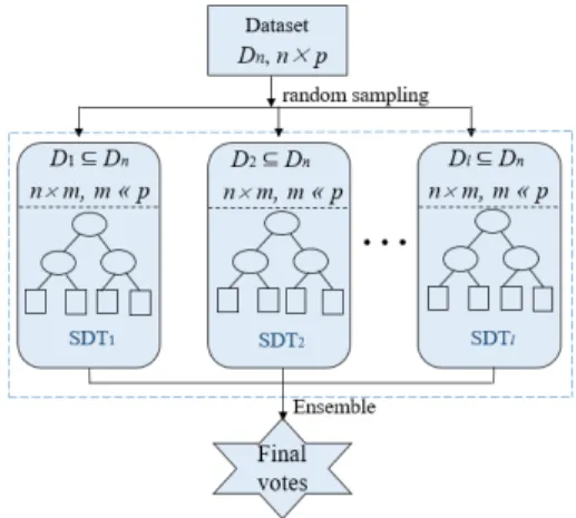
Fig. 1. The flow graph of the random Shapley forests algorithm.
According to this rule, we evaluate the Shapley value for each feature to determine its importance at each node of SDTs.
Furthermore, Shapley value has some particularly attractive properties, i.e., the group effectiveness, the symmetry and the additivity [22]. The group effectiveness can lead the proposed random forest algorithm (RSFs) to obtain the consistency, which can be defined as follows.
X
i∈N
βi(Γ) =γ(N). (3)
By the group effectiveness Eq. (3), we can normalize the Shapley value of each member (player)βi(Γ)to
φi(Γ) =
βi(Γ)
P
i∈Nβi(Γ)
. (4)
For the RSFs, we use the Shapley value to evaluate the importance of candidate features at each node of SDTs. In this context, each step of decision tree construction can be regarded as a cooperative game, where each feature can be regarded as a player in a cooperative game. In particular, Shapley value has been proved to be effective in assessing the importance of features [43]. It can not only provide a fair way to estimate the importance of each candidate feature but also consider the possible intrinsic and intricate correlative interactions among features.
B. Construction of SDTs
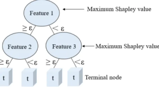
At each node of the SDTs, SDTs combine the Shapley value to evaluate the importance of the candidate features. Among the candidate features, we specify that the candidate feature with the maximum Shapley value is strong, otherwise weak. Then, the strong feature is selected as a node feature, and the corresponding midpoint value as the split threshold. If there are more than one strong features, then a feature is randomly selected and split. A single SDT will stop growing, when a tree node has a small amount of samples or the SDTs reaches a fixed number of splits. Specifically, the construction of SDTs is given in Fig. 2.
More specifically, the details of the feature evaluation method based on the Shapely value are described as follows.
Fig. 2. A Shapley decision tree.
The construction of SDTs can be treated as a cooperative game Γ = (N, γ), which is composed of a feature player set
N ={f1, . . . , fn}. From the Eq. (1), if we want to obtain the Shapley value of the featurefi(i∈(1,2, . . . , n)), we must first know the number of coalitions S ⊆ N with revenue growth. That is, the number of coalitions in which a feature fi(i ∈
(1,2, . . . , n)) is added to an arbitrary coalition to increase the revenue of the joined coalition S ⊆ N. Therefore, we specify whether the featurefi(i∈(1,2, . . . , n))can lead to a coalitionSgaining more revenue can be measured by the ratio σ =µfi(S)/ρfi(S), where µfi(S)represents the number of
features (belonging to the coalitionS) that interdependent with the features fi ∈ S/ (i ∈(1,2, . . . , n)), and ρfi(S)represents
the total number of features in the coalition S. We define that when σ≥1/2, then the featurefi∈ S/ , i∈(1,2, . . . , n)can increase the revenue of a coalition S. The formula is
∆i(S) =γ(S ∪ {i})−γ(S) =
1 σ≥1/2;
0 σ <1/2. (5) The ratio σ ≥ 1/2 means that more than half of the features (belonging to the coalition S) are interdependent with fi, then fi joining S) can make the revenue of the coalition S to increase. Here, the conditional mutual information [44] is employed to measure the interdependence between the feature fi ∈ S/ and the feature fj ∈ S. The corresponding formula is
I(fi;y|fj) =p(fi, fj,y) log
p(fi,y|fj) p(fi|fj)p(y|fj)
, (6)
where the vector y represents the target class. The featurefi andfj are interdependent. The relevance between the feature fi and the target classy can be increased conditioned on the feature fj, i.e. I(fi;y) ≤ I(fi;y|fj). I(fi;y) = p(fi,y) log
p(fi,y)
p(fi)p(y) is the mutual information
between the feature fi and the target class y.
Therefore, by Eqs. (4) and (6), we can obtain the Shapley value of each candidate feature. Furthermore, this computational process is described in Algorithm 1.
C. Random Shapley forests
Random Shapley forests (RSFs) consist of several Shapley decision trees (SDTs) based on the bagging method [16]. The algorithm flow of RSFs is demonstrated in Fig. 1. Moreover, the algorithm details of RSFs are presented in Algorithm 2.
From Fig. 1 and Algorithm 2, it is not difficult to find that the RSFs has a similar architecture to the existing consistent
Algorithm 1: Evaluating the importance of candidate features using the Shapley value
Input: Given a training data setDnwith feature spaceN and the data labelsy,β=0.
Output:φ: the Shapley value vector ofN.
Foreach featurefi∈ N do
Create the coalitions set{S1, . . . ,St}overN \ {fi};
Foreach coalitionSj∈ {S1, . . . ,St}do Calculate the marginal function∆fi(Sj)based on
Eq.(5) and Eq.(6).
End
Calculate the Shapley valueβfiusing Eq.(1); End
Normalize the Shapley valueβfiusing Eq.(4) to obtainφfi;
Algorithm 2: Random Shapley Forests (RSFs)
Given a set ofnlabeled training samplesDn={(x1, y1), . . . , (xn, yn)}with each candidate featurefj= (x1,j, . . . ,xn,j)T, j= 1, . . . , p.
Forl= 1, . . . , L,
1. Take the samplesDlof sizenfromDnwith replacement; 2. For each SDTs, select at random, without replacementmp
features as the candidate features. Moreover, for each node, the Shapley value is used to evaluate the strength or weakness of mpcandidate features, then the strongest featurefjis selected, and the midpoint value of the featurefjis the splitting threshold.
i. If there is more than one strong feature selected, choose one at random and split.
Repeat step 2 until reaching the user-set limit, i.e., a minimal number of samples at a node or a fixed number of splits.
3. RSFs predict the class label of a test samplexaccording to the most votes received from the SDTsl,(l= 1, . . . , L).
random forests algorithm (called Biau12) [21]. That is, they are all select the midpoint of the strong feature as the split threshold. The main difference between the Biau12 and RSFs lies in RSFs use the Shapley value to assess the strength or weakness based on a fixed number of candidate features at each tree node, and Biau12 firstly evaluates the power or importance of all candidate features of data samples, then selects the strong feature as the node feature.
However, Biau12 pays close attention to the consistency of the algorithm, which does not resort an effective method to evaluate the power of candidate features [21]. In this paper, we explore an unbiased and effective way to estimate the importance of the features while considering the features possible intrinsic correlation.
D. Computational complexity
To evaluate the power of the candidate features, it is necessary to calculate the proportion of the revenue increase coalitions according to Eqs. (2) and (1). Theoretically, calculating the Shapley value requires summing over all possible feature subsets, which may lead to high computational complexity. However, it is unnecessary to consider empty-set and large coalitions. By the Eq. (5), there is a very small probability that a single feature fi can increase the revenue of a large coalition. Therefore, we set a bound $ to limit the size of coalitions. That is, to limit the number of features in the coalitions. To the end, Eq. (1) can
be redefined as βi(Γ) = X S⊆Π$ ∆i(S) |S|!(n− S −1)! n! , (7)
whereΠ$ is the subset of the feature setF\ {fi}.
For the proposed algorithm, whether a coalition’s revenue increase or not depends on the number of features increasing (or reducing) its associate with the target class when the condition is given. Therefore, at each node of SDTs, the number of coalitions with increased revenue containing only one feature player (denoted as M1) that can be calculated
with time complexity O(n), where ndenotes the number of features at a tree node. Moreover, we can use the knowledge of combinatorial mathematics and dynamic programming [45] to calculate the number of coalitions with increased revenue that including more than one feature player based on M1. For example, M2 calculate as
M2 = CM21 +C
1
M1 ×C
1
n−M1, where C is the number of combinations. In this way, we can construct each SDT with low computational complexity in RSFs.
In the experiment, we use 5-fold cross-validation to determine the value of$. When$ ∈[3,6], the performance of RSFs is satisfactory. Thus, we suggest $ ∈[3,6] in most applications.
IV. CONSISTENCY OFRSFS
We first define the prediction function of RSFs before introducing the consistency of RSFs. RSFs predict the class of the test sample x according to the most votes received from a fixed number of SDTs. For each SDT, it can obtain the classification prediction gk
n(x)of the test sample x. That is gnk(x) = 1 N(An(x)) X (Xi,Yi)∈An(x) δ(Yi=k),
whereY is a multi-class random variable,An(x)denotes the terminal node that contains x, and N(An(x)) is the number of samples that locate in An(x). Moreover, the predicting of single SDT is
f(x) = arg max
y (g k n(x)).
From the prediction of RSFs, the consistency of RSFs can be obtained by the consistency of each SDT. As the samplen varies, we can obtain a sequence of SDTs in RSFs, i.e.{gk
n}. Then, we only need to prove the base tree classifier sequence
{gnk} is consistency. According to the work of Devroye et al. on the consistency of decision trees [46], we define that a sequence {gkn} of SDTs classifiers is consistent, when the probability error ofgnk converges to the Bayes riskL∗, i.e. as n→ ∞, have
L(gnk) =p(gnk(X, θ, Dn)6=Y)→L∗,
where (X, Y) is a random test data sample, Dn denotes the training data and θ represents the randomness on the constructing SDTs, such as randomly select a fixed number of features at each node. The Bayes risk L∗ represents the minimum prediction error of the Bayes classifier on the
distribution of(X, Y), which makes predictions by choosing a class that have the highest posterior probability, g(x) = arg max
k p(Y =k|X=x).
Moreover, RSFs and the corresponding SDTs are the multi-class classifiers. We can convert the multi-class classifier into a number of two-class classifiers. i.e. given a set of classes {1,2, . . . , c}. We can then re-assign the labels by employing the map (X, Y) 7→ (X,I(Y =k)) for any k ∈ {1, . . . , c}. Then, solving a two-class classification problem gn(x) = p(Y = 1|X = x) is equivalent to learn gk
n(x) in the original multi-class classification problem. Therefore, the problem is converted to proof that the sequence of SDTs classifiers {gn} is consistent for the corresponding two-class problem. For this situation, as the number of SDTs tends to be infinite, the proposed RSFs take a majority vote to obtain classification results, which can well approximation by the averaged classifier according to the Proposition 1 of Biauet al.[20]. Therefore, we recall the Proposition 1 of Biauet al. [20] as Lemma 1.
Lemma 1 Assuming the sequence {gn} of tree classifiers is consistent under a certain distribution of(X, Y). Then, the voting random forests classifier gn(l) (for any value of l, l represents the number of trees) and the averaged random forests classifiergn are also consistent.
Proof. See that for Proposition 1 of Biauet al.. [20]. Thus, we give the consistency result of RSFs for the averaged classifiergn according to the Lemma 1.
Before introducing the main theorem, some parameter settings are declared about the construction of each SDTs in RSFs. We rule that the individual SDTs stop growing when each SDT has exactly 2dlog2kne(≈ k
n) terminal nodes. Accordingly, each terminal node has Lebesgue measure
2−dlog2kne(≈ k
n). Therefore, if the sample set X has uniform distribution on [0,1]p, there will be an average of n/kn observations on each terminal node. Whenkn =n , it will induce a very small number of samples in the terminal nodes. In fact, there is similar and different between the construction of the proposed RSFs model and the Biau et al.’s consistency model (it is called Biau12) [21]. That is, both of the them select the midpoint of the node feature as the location of the node splitting. In particular, in order to exclude any data-dependent strategy in the process of building each tree, Biau et al. [21] use a second dataset (it has the same size and distribution as the train dataset) to evaluate the node features. However, the method of evaluating features is not given in the Biau12. Moreover, to obtain the consistency of RSFs, we assume that using the Shapley value to evaluate each candidate feature of the dataset Dl ⊆ Dn based on a second dataset D
0
l, where D
0
l and Dl ⊆ Dn has the same size and distribution. The purpose for that is to exclude any data-dependent strategy to build each SDTs in RSFs. Therefore, inspired by the work of Biau et al. [21], the main Theorem result is given as following.
Theorem 1 Assuming the distribution of X has support on [0,1]p ⊆ Dn. Then the RSFs estimate gn is consistent whenever pnjlog2kn → ∞ for all j = 1,2, . . . , p and
kn/n → 0 as n → ∞, where pnj is a normalized Shapley value of the j-th candidate feature.
Proof. By Lemma 1, the consistency of RSFs can be obtained by the consistency of each SDT. Therefore, we can only show that the sequence {gn} of SDTs is consistent for the corresponding two-class problem.
To prove the consistency of each SDT, we employ the consistency theorem of the tree classifiers in [46] (Gy¨orfi et al., 1996, Theorem 6.1). According to Theorem 6.1, the SDTs classifier gn is consistent, if both diam(An(X, θ))→ 0 in probability and Nn(X, θ)→ ∞ in probability, where An(X, θ) represents the tree node that containing sampleX and
Nn(X, θ) = n
X
i=1
I{Xi∈An(X,θ)}
denotes the number of the samples falling in the same node as X.
The proof ofNn(X, θ)→ ∞ in probability is the same as that of the Theorem 1 of Biauet al. [21].
It remains to show thatdiam(An(X, θ))→0in probability. To this goal, we only need to show the size of each feature in the tree nodeAn(X, θ)tend to 0. Moreover, theVnj(X, θ)is defined to denote the size of thej−thfeature in the tree node An(X, θ). Then, it suffices to show that Vnj(X, θ) → 0 in probability for all the featuresj= 1,2, . . . , p. LetKnj(X, θ) be the number of times that the tree node containingXis split when we construct the SDTs partition.
Let Knj(X, θ) be binomial B(log2kn,pnj) distribution, representing the number of times the tree node containing x is split along the j−th feature. pnj is the Shapley value of the j-th feature. Then, Vnj(X, θ) = 2−Knj(X,θ). Clearly, it suffices to show that Vnj(X, θ)→0 in probability for all the features j = 1,2, . . . , p, so it is enough to show that for all X,E[Vnj(X, θ)]→0. Thus,
E[Vnj(X, θ)] =E[2−Knj(X,θ)]
=E[E[2−Knj(X,θ)|X]]
= (1−pnj/2)dlog2kne,
which tends to 0 as pnjlog2kn → ∞, wherepnj =φj is a normalized Shapley value of thej-th feature.
By Lemma 1 and Theorem 1, the consistency of RSFs is proved for the multi-class. Note that, the bagging method is used to sample data samples for construction each SDT in RSFs. According to the work of Biauet al. [20], the random forest model that integrates with bagging method is consistent, when the base tree classifier has consistency (see Theorem 6 [20]). Therefore, RSFs integrated with bagging method, which remains consistent.
V. EXPERIMENT
To demonstrate the effectiveness of RSFs, we evaluated RSFs on eight UCI benchmark datasets and four real-world datasets. In particular, we show the difference between the traditional method of evaluating features and the Sharpley value in terms of the select node features in building a decision tree.
A. Datasets
Four real-world datasets are employed in the experiments, they are the 20Newsgroups dataset1, USPS dataset2, Yale dataset3, and CMU mocap dataset [47]. Moreover, we use eight datasets from the UCI machine learning repository [48] to verify the performance of RSFs. These datasets come from a variety of application domains, such as text classification, face recognition, human pose estimation, medical diagnosis, and physical analysis etc. Table I shows the properties of these twelve datasets. The feature dimensions of these datasets range from tens to thousands. In particular, the human pose estimation data (CMU mocap dataset) choose 49 video sequences from four subjects, which includes three categories, walking, running and jumping. For each sequence, the feature are generated using Lawrence’s method4, with dimensionality 93.
TABLE I
SUMMARY OF THE USED DATASETS.
Dataset No.examples No.features No.classes
CMU mocap 49 93 3 Yale 165 1024 15 dermatology 366 34 6 attfaces 400 10304 40 housing 506 13 2 cancer 569 30 2 vehicle 846 18 4 waveform21 5000 21 3 isolet 6238 617 26 musk2 6598 166 2 usps 9298 256 10 20newsgroups 16242 100 4 B. Classification performance
We compare the RSFs with the existing consistent random forests (Biau12) [21], the non-consistent original random forests (RFs) [16] and a well-known classifier: the support vector machines (SVMs) [49] in terms of the classification accuracy. Moreover, SVMs used the radial basis function (RBF) kernel; Biau12 firstly evaluates the importance of all candidate features of the training dataset before constructing the trees. Then, at each node, select at random, with replacement, a small number of candidate features to split on. If the selection is all weak, then choose one at random to split on. If there is more than one strong variable elected, choose one at random and split. The split threshold is the midpoint value of the chosen feature. Stop building a tree in Biau12 when the node contains only one sample. Here, both RFs and the Biau12 algorithm used the information gain ratio to evaluate candidate features for each tree node. Although the Gini index was also employed in RFs [16], the information gain ratio based evaluation method occupied the dominant position in random forest algorithms.
For all the random forests, the number of trees was empirically set to be 100, i.e., l = 100. For each individual
1http://qwone.com/ jason/20Newsgroups/
2http://statweb.stanford.edu/ tibs/ElemStatLearn/data.html 3http://cvc.cs.yale.edu/cvc/projects/yalefaces/yalefaces.html 4http://is6.cs.man.ac.uk/ neill/mocap/
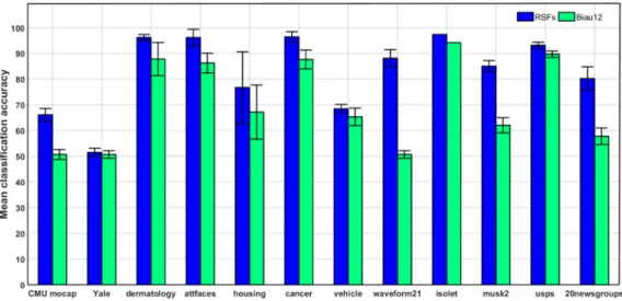
Fig. 3. Mean classification accuracy and standard deviations obtained by comparing RSFs with Biau12. For all algorithms, 5-fold cross-validation was implemented to determine the parameters.
tree, m = round(log2(p) + C) candidate features were randomly chosen, where p was the feature dimensional of the samples and C ∈ R was a parameter. For all of the
algorithms, 5-fold cross-validation was applied to optimize the parameters.
The experimental results are shown in Table II. For each dataset, the classification result was obtained by averaging over 5-fold cross-validation except for the isolet dataset. The training and test partition of the isolet dataset was given in advance. The boldface items represent the best performance. It can be seen from Table II that the performance of RSFs is better than that of other algorithms on the majority of datasets. Moreover, to compare the algorithms performance in a scientific and reasonable manner, we used the Friedman and Nemenyi statistical test [50] for comparison of four classifiers over twelve datasets, CD = 1.3540. As show in Table II, the mean rank of four classifiers was obtained. The evaluation criterion is that the lower mean rank the better performance of the classifier. Based on Friedman and Nemenyi statistical test, the performance difference of the classifiers are significant. In particular, the performance difference of Biau12 [21] and RSFs is significant, i.e. see Fig. 3. The results of the Fig. 3 imply that RSFs combined the Shapley value to evaluate the importance of candidate features at each node, which can consider the possible intrinsic correlation between features for the target classes. However, RFs and Biau12 used the information gain ratio to evaluate the importance of candidate features, the information gain ratio tends to select the feature with a strong discriminate ability and often pays less attention to the intrinsic structure of candidate features. Thus, any combination of predicting candidate features which represents a much stronger prediction may be lost [51].
C. Performance analysis
To clarify the effect of the shapley value and the information gain ratio on the performance of random forests. We show the results of feature selection on a tree by using
the different splitting node methods based on the cancer dataset, as shown in Fig. 4. Note that, the relevance of the feature and the target class can be calculated by the mutual information. Moreover, the interdependence among features can be calculated by the conditional mutual information. From the Fig. 4, we can see that the RFs use the information gain ratio method to select feature with the high relevance (strong discriminate ability) for each tree node. Nevertheless, the proposed RSFs use the Shapley value to select feature with the low relevant, but these features are highly interdependent in terms of target classes. In fact, some practical classification problems require a certain number of features to interpret it. Meanwhile, the individual feature of this certain number of features is not very strong, but they have the strong discriminatory ability when they combined. For solving such problems, the RSFs algorithm is effective. For example, the attfaces dataset and musk2 dataset. This reason also illustrates why the RSFs perform poor on the attfaces dataset and musk2 dataset.
Fig. 4. The results of feature selection on a tree by using the different splitting node methods based on the cancer dataset.
D. Effect of the parameters
There are two parameterslandmin the RSFs. Whereland mrepresents the number of Shapley decision trees (SDTs) and the number of randomly selected candidate features for each SDTs, respectively. Here, we used two datasets to verify the
TABLE II
MEAN CLASSIFICATION ACCURACY AND STANDARD DEVIATIONS OBTAINED BY COMPARINGSVMS WITH RANDOM FORESTS. ALGORITHMS WITH THE BEST ACCURACY IS SHOWN IN BOLDFACE.
Dataset SVMs RFs Biau12 RSFs CMU mocap 0.5239±0.0210 0.6878±0.0177 0.5069±0.0194 0.6612±0.0241 Yale 0.7400±0.1362 0.5156±0.0183 0.5067±0.0147 0.5147±0.0163 dermatology 0.9540±0.0130 0.9530±0.0167 0.8777±0.0643 0.9617±0.0117 attfaces 0.8800±0.0527 0.9800±0.0227 0.8625±0.0385 0.9613±0.0324 housing 0.7605±0.1151 0.6418±0.0645 0.6715±0.1052 0.7673±0.1385 cancer 0.8629±0.0234 0.9526±0.0230 0.8763±0.0368 0.9642±0.0200 vehicle 0.6728±0.0470 0.6490±0.0076 0.6532±0.0340 0.6843±0.0172 waveform21 0.8630±0.0117 0.8406±0.0129 0.5067±0.0147 0.8810±0.0338 isolet 0.9628±0.0000 0.9529±0.0000 0.9415±0.0000 0.9735±0.0000 musk2 0.8508±0.0747 0.8546±0.1204 0.6202±0.0292 0.8501±0.0022 usps 0.9251±0.0132 0.9041±0.0183 0.8968±0.0126 0.9317±0.0115 20newsgroups 0.7872±0.0580 0.7729±0.0579 0.5776±0.0323 0.8023±0.0455 mean rank 2.2500 2.5000 3.7500 1.5000
(a) housing (b) dermatology
Fig. 5. Relationship between the number of SDTs and the performance on housing and dermatology.
(a) housing (b) dermatology
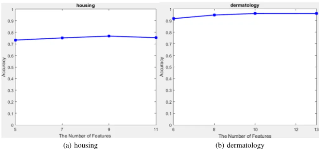
Fig. 6. Relationship between the number of features and the performance on housing and dermatology.
parameter robustness of RSFs, i.e., housing and dermatology. The properties of the two datasets can be found in Table I. For other datasets, RSFs can obtain the same or similar results, therefore, we only give the results of the two datasets.
For the parameter l, we set that the value ofl was selected from a set of{5,10,50,100,500}. The parametermwas fixed at 2√p in this experiment. The results are shown in Fig. 5. We can see that the classification accuracy increases gradually with the increasing of the number of SDTs. In particular, when the value of l is larger than 50, a good prediction can be
obtained. This indicates that RSFs will not incur over-fitting. Moreover, this result also justifies that it is reasonable to fix the number of SDTsl at100 in our experiments.
To verify the robustness of the parameter m in RSFs, we first fixed the number of SDTs l equal to 100, i.e., l = 100. Then, as the number of features increases, we observe the performance of RSFs. From the Fig. 6, we can see that the RSFs obtains the best performance, when the number of features m is approach to 10. The result demonstrates that RSFs are robust to the parameter m. By this fact, we can
save much time to tune parameter.
E. Consistency verification
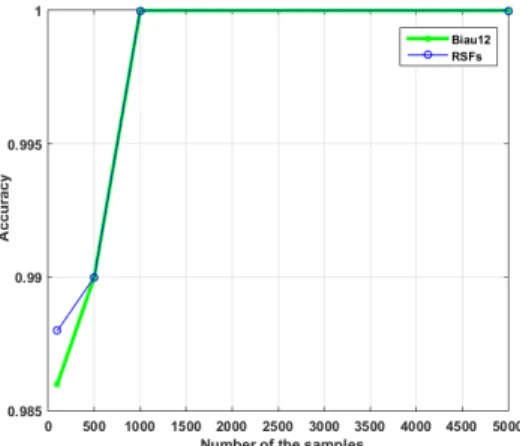
In this section, we verify the consistency of RSFs on the artificial dataset. The consistency indicates whether the algorithm could converge to an optimal solution as the sample size tends to infinity. Thus, the performance of the consistency algorithms, Baiu12 [21] and RSFs, should approach each other with an increase in the number of samples. To verify this fact, we generated the artificial dataset with three different classes of eight-dimensional Gaussian distributed data samples whose means are µ =
{(0,0,0,0,0,0,0,0),(4,4,4,4,4,4,4,4),(−4,−4,−4,−4,−
4,−4,−4,−4)} and variances are σ2 = 1,1,1 with on covariance between eight dimensions. To verify the performance of Biau12 and RSFs, we set that the number of training samples of each class was selected from a set of
{100,500,1000,5000}. The number of test samples was 100. Moreover, for the Biau12 and RSFs, the number of trees was set to be 100. m=round(log2(p) + 1) candidate features were randomly chosen at each individual tree, where p = 8 was the feature dimensional of the samples. The results of the consistency algorithms on the artificial dataset are shown in Fig. 7. From the Fig. 7, it can be easily noticed that the classification accuracy of Biau12 and RSFs is gradually increasing and approach each other as the number of training samples increases. Finally, both Biau12 and RSFs obtain the best accuracy.
Fig. 7. The classification performance of Biau12 and RSFs on the artificial dataset.
VI. CONCLUSION
The original random forests algorithm is an effective tool for the classification and regression. So far, many variants have emerged. For existing random forests with consistency, it is hard to find an off-line classification algorithm that not only has the theoretical guarantee but also has a good performance. The majority of algorithms use the information theory to find the optimal split threshold, which often tends to pay less attention to the dependencies between the candidate features at each tree node. Therefore, a combination of the candidate features which represents a
strong prediction may be missed [52]. The Shapley value from the cooperative game can not only capture this relationship but also evaluate the importance of the features fairly and reasonably. Accordingly, we propose a novel random forests algorithm with consistency, called random Shapley forests (RSFs). The advantage of RSFs is that it is a random forest classification algorithm with good classification accuracy and theoretical consistency. The disadvantage of RSFs is that the running time is longer than the original random forests algorithm. Fortunately, the running time of the RSFs is acceptable by analyzing the computational complexity. In the future, we will try to combine the RSFs and the existing neural networks to explore the internal relationship between features.
ACKNOWLEDGEMENTS
This work was supported by the Major Project for New Generation of AI under Grant No. 2018AAA0100400, the National Natural Science Foundation of China (NSFC) under Grant No. 41706010, the Science and Technology Program of Qingdao under Grant No. 17-3-3-20-nsh, the CERNET Innovation Project under Grant No. NGII20170416, the Joint Fund of the Equipments Pre-Research and Ministry of Education of China under Grand No. 6141A020337, the Open Fund of Engineering Research Center for Medical Data Mining and Application of Fujian Province under Grand No. MDM2018007, and the Fundamental Research Funds for the Central Universities of China.
REFERENCES
[1] F. Schwenker, “Ensemble methods: Foundations and algorithms [book review],” IEEE Computational Intelligence Magazine, vol. 8, no. 1, pp. 77–79, 2013. [2] L. Rokach, “Ensemble-based classifiers,” Artificial
Intelligence Review, vol. 33, pp. 1–39, 2010.
[3] L. K. Hansen and P. Salamon, “Neural network ensembles,”IEEE Transactions on Pattern Analysis and Machine Intelligence, vol. 12, no. 10, pp. 993–1001, 2002.
[4] M. F. Amasyali, “Improved space forest: A meta ensemble method,” IEEE Transactions on Cybernetics, vol. 49, no. 3, pp. 816–826, 2019.
[5] L. Zhang and P. N. Suganthan, “Oblique decision tree ensemble via multisurface proximal support vector machine,” IEEE Transactions on Cybernetics, vol. 45, no. 10, pp. 2165–2176, 2015.
[6] W. Wu, Y. Yin, X. Wang, and D. Xu, “Face detection with different scales based on faster r-cnn,”IEEE Transactions on Cybernetics, vol. 49, no. 11, pp. 4017–4028, 2019. [7] T. Zhang, W. Zheng, Z. Cui, Y. Zong, and Y. Li,
“Spatialctemporal recurrent neural network for emotion recognition,”IEEE Transactions on Cybernetics, vol. 49, no. 3, pp. 839–847, 2019.
[8] G. Zhong, H. Yao, Y. Liu, C. Hong, and T. Pham, “Classification of photographed document images based on deep-learning features,” in Eighth International
Conference on Graphic and Image Processing (ICGIP 2016), 2017, pp. 176–181.
[9] J. Sun, G. Zhong, Y. Chen, Y. Liu, T. Li, and K. Huang, “Generative adversarial networks with mixture of t-distributions noise for diverse image generation,”Neural Networks, vol. 122, no. 12, pp. 374–381, 2020.
[10] L. Duan, S. Ma, C. Aggarwal, T. Ma, and J. Huai, “An ensemble approach to link prediction,” IEEE Transactions on Knowledge and Data Engineering, vol. 29, no. 11, pp. 2402 – 2416, 2017.
[11] A. Bagnall, J. Lines, J. Hills, and A. Bostrom, “Time-series classification with cote: The collective of transformation-based ensembles,”IEEE Transactions on Knowledge and Data Engineering, vol. 27, no. 9, pp. 2522–2535, 2015.
[12] S. Wang, L. L. Minku, and X. Yao, “Resampling-based ensemble methods for online class imbalance learning,”
IEEE Transactions on Knowledge and Data Engineering, vol. 27, no. 5, pp. 1356–1368, 2015.
[13] S. Scardapane and L. P. Di, “A framework for parallel and distributed training of neural networks.” Neural Networks, vol. 91, pp. 42–54, 2017.
[14] M. Amozegar and K. Khorasani, “An ensemble of dynamic neural network identifiers for fault detection and isolation of gas turbine engines,” Neural Networks, vol. 76, pp. 106–121, 2016.
[15] S. Scardapane and P. D. Lorenzo, “A framework for parallel and distributed training of neural networks,”
Neural Networks, vol. 91, pp. 42–54, 2017.
[16] L. Breiman, “Random forests,” Machine Learning, vol. 45, no. 1, pp. 5–32, 2001.
[17] H. Liang, J. Yuan, J. Lee, L. Ge, and D. Thalmann, “Hough forest with optimized leaves for global hand pose estimation with arbitrary postures,” IEEE Transactions on Cybernetics, vol. 49, no. 2, pp. 527–541, 2019. [18] M. Ristin, M. Guillaumin, J. Gall, and L. V. Gool,
“Incremental learning of random forests for large-scale image classification,” IEEE Transactions on Pattern Analysis and Machine Intelligence, vol. 38, no. 3, pp. 490–503, 2016.
[19] A. Gonzlez, D. Vzquez, A. M. Lpez, and J. Amores, “On-board object detection: Multicue, multimodal, and multiview random forest of local experts,” IEEE Transactions on Cybernetics, vol. 47, no. 11, pp. 3980– 3990, 2017.
[20] G. Biau, L. Devroye, and G. Lugosi, “Consistency of random forests and other averaging classifiers,” Journal of Machine Learning Research, vol. 9, pp. 2015–2033, 2008.
[21] G. Biau, “Analysis of a random forests model,” Journal of Machine Learning Research, vol. 13, no. 1, pp. 1063– 1095, 2012.
[22] L. S. Shapley, “A value for n-person games,”
Contribution to the Theory of Games II, Princeton University Press, Princeton, pp. 307–317, 1953. [23] R. R. Yager, “On using the shapley value to approximate
the choquet integral in cases of uncertain arguments,”
IEEE Transactions on Fuzzy Systems, vol. 26, no. 3, pp.
1303–1310, 2018.
[24] W. Loh, “Classification and regression trees,” Wiley Interdisciplinary Reviews-Data Mining and Knowledge Discovery, vol. 1, no. 1, pp. 14–23, 2011.
[25] S. L. Salzberg, “C4.5: Programs for machine learning by j. ross quinlan. morgan kaufmann publishers, inc., 1993,”
Machine Learning, vol. 16, no. 3, pp. 235–240, 1994. [26] T. K. Ho, “The random subspace method for constructing
decision forests,”IEEE Transactions on Pattern Analysis and Machine Intelligence, vol. 20, no. 8, pp. 832–844, 1998.
[27] ——, “Random decision forests,” in International Conference on Document Analysis and Recognition, vol. 1, 1995, pp. 278–282.
[28] T. G. Dietterich, “An experimental comparison of three methods for constructing ensembles of decision trees: Bagging, boosting, and randomization,” Machine Learning, vol. 40, no. 2, pp. 139–157, 2000.
[29] N. Meinshausen, “Quantile regression forests,”Journal of Machine Learning Research, vol. 7, pp. 983–999, 2006. [30] H. Ishwaran, U. B. Kogalur, E. H. Blackstone, and M. S. Lauer, “Random survival forests,”The Annals of Applied Statistics, vol. 2, no. 3, pp. 841–860, 2008.
[31] S. Clmencon, “Ranking forests,” Journal of Machine Learning Research, vol. 14, no. 1, pp. 39–73, 2010. [32] N. Quadrianto and Z. Ghahramani, “A very simple
safe-bayesian random forest,” IEEE Transactions on Pattern Analysis and Machine Intelligence, vol. 37, no. 6, pp. 1297–1303, 2015.
[33] J. Sun, G. Zhong, J. Dong, H. Saeeda, and Q. Zhang, “Cooperative profit random forests with application in ocean front recognition,” IEEE Access, vol. 5, no. 99, pp. 1398–1408, 2017.
[34] J. Shotton, A. Fitzgibbon, M. Cook, T. Sharp, M. Finocchio, R. Moore, A. Kipman, and A. Blake, “Real-time human pose recognition in parts from single depth images,” in Computer Vision and Pattern Recognition, 2011, pp. 1297–1304.
[35] Z. S. Wei, J. Y. Yang, H. B. Shen, and D. J. Yu, “A cascade random forests algorithm for predicting protein-protein interaction sites,” IEEE Transactions on Nanobioscience, vol. 14, no. 7, pp. 746–760, 2015. [36] L. Zhang, Q. Wang, Y. Gao, G. Wu, and D. Shen,
“Concatenated spatially-localized random forests for hippocampus labeling in adult and infant mr brain images,” Neurocomputing, vol. 229, no. 15, pp. 3–12, 2017.
[37] M. Denil, D. Matheson, and N. D. Freitas, “Consistency of online random forests,” inInternational Conference on International Conference on Machine Learning, vol. 28, 2013, pp. 1256–1264.
[38] H. Ishwaran and U. B. Kogalur, “Consistency of random survival forests,” Statistics and Probability Letters, vol. 80, pp. 1056–1064, 2010.
[39] R. Zhu, D. Zeng, and M. R. Kosorok, “Reinforcement learning trees,” Journal of the American Statistical Association, vol. 110, no. 512, pp. 1770–1784, 2015. [40] R. Genuer, “Variance reduction in purely random
forests,” Journal of Nonparametric Statistics, vol. 24, no. 3, pp. 543–562, 2012.
[41] M. Wooldridge, “Computational aspects of cooperative game theory,” Synthesis Lectures on Artificial Intelligence and Machine Learning, vol. 5, no. 6, pp. 139–152, 2011.
[42] A. E. Roth and L. S. Shapley, “The shapley value : essays in honor of lloyd s. shapley,”Economic Journal, vol. 101, no. 406, pp. 235–264, 1988.
[43] S. Xin, Y. Liu, L. Jin, J. Zhu, X. Liu, and H. Chen, “Using cooperative game theory to optimize the feature selection problem,”Neurocomputing, vol. 97, no. 15, pp. 86–93, 2012.
[44] S. Phoenix, “Elements of information theory,”Journal of the American Statistical Association, vol. 39, no. 7, pp. 1600–1601, 1992.
[45] T. H. Cormen, C. E. Leiserson, R. L. Rivest, and C. Stein,
Introduction to Algorithms. The MIT Press, 2009. [46] L. Devroye, L. Gy¨orfi, and G. Lugosi, A Probabilistic
Theory of Pattern Recognition. Springer-Verlag, New York, 1996.
[47] G. Zhong, W. Li, D. Yeung, X. Hou, and C. Liu, “Gaussian process latent random field,” in Proceedings of the Conference on Artificial Intelligence AAAI, 2010, pp. 679–684.
[48] C. Blake, “Uci repository of machine learning databases,” p. https://archive.ics.uci.edu/ml/datasets.html, 1998. [49] C. Chang and C. Lin, “Libsvm: A library for support
vector machines,” ACM Transactions on Intelligent Systems and Technology, vol. 2, no. 3, p. 27, 2011. [50] J. Demisar and D. Schuurmans, “Statistical comparisons
of classifiers over multiple data sets,”Journal of Machine Learning Research, vol. 7, no. 1, pp. 1–30, 2006. [51] J. N. Morgan and R. C. Messenger, “Thaid, a sequential
analysis program for the analysis of nominal scale dependent variables,”Isr, 1973.
[52] M. A. Muharram and G. D. Smith, “Evolutionary feature construction using information gain and gini index,” in
Eurogp, 2004, pp. 379–388.
Jianyuan Sun received her BSc from the Department of Applied Mathematics at Ocean University of China in 2010. She received her Ph.D. degree in Computer Application Technology in June 2019, from the College of Information Science and Engineering at Ocean University of China. She is currently a research associate at the National Centre for Computer Animation, Bournemouth University, Poole, UK. She research interests include deep learning, machine learning, computer vision and 3D reconstruction.
Hui Yu is Professor with the University of Portsmouth, UK. He used to work at the University of Glasgow before moving to the University of Portsmouth. His research interests include methods and practical development in vision, machine learning and AI with applications to human-machine interaction, Virtual and Augmented reality, robotics and geometric processing of facial expression. He serves as an Associate Editor of IEEE Transactions on Human-Machine Systems and Neurocomputing journal.
Guoqiang Zhong received the
Ph.D. degree in 2011 from Institute of Automation, Chinese Academy of Sciences (CASIA), Beijing, China. Between October 2011 and July 2013, he was a Postdoctoral Fellow with the Synchromedia Laboratory for Multimedia Communication in Telepresence, Ecole de Technologie Superieure (ETS), University of Quebec, Montreal, Canada. Since March 2014, he has been an associate professor at Department of Computer Science and Technology, Ocean University of China, Qingdao, China. He won the outstanding reviewer award of the Pattern Recognition journal for 2014 and 2015.
Junyu Dong received the
Ph.D. degree in 2003 from Heriot-Watt University, UK. Junyu Dong joined Ocean University of China in 2004. From 2004 to 2010, Dr. Junyu Dong was an associate professor at the Department of Computer Science and Technology. He became a Professor in 2010 and is currently the Head of the Department of Computer Science and Technology. Currently, Prof. Dong is the Chairman of Qingdao Young Computer Science and Engineering Forum (YOCSEF Qingdao). He is a member of ACM and IEEE. Prof. Dongs research interests include texture perception and analysis, 3D reconstruction, video analysis and underwater image processing.
Shu Zhang
received his PhD degree in Computer Application Technologies from Ocean University of China, Qingdao, China. He was a research associate at University of Portsmouth, Portsmouth, UK. He is currently a lecturer with Ocean University of China, Qingdao, China. His main research interests include image processing, feature matching, 3D reconstruction, underwater image analysis.
Hongchuan Yureceived his BSc and MSc degree in University of Science and Technology of China, Hefei, and Ph.D. Degree in Computer Vision from the Institute of Intelligent Machine, Chinese Academy of Sciences, Beijing, PRC, in 2000.
He is currently
an Academic Principal at the National Centre for Computer Animation, Bournemouth University, Poole, UK. His research interests include Geometry modeling and rendering, data mining with applications to graphics and image processing.