Characterizing bladder cancer cells by comparing general machine learning methods to convolutional neural network

(1)

Theses

3-5-2019

Characterizing bladder cancer cells by comparing

general machine learning methods to convolutional

neural network

Peng Nien Yin

[email protected]

Follow this and additional works at:

https://scholarworks.rit.edu/theses

This Thesis is brought to you for free and open access by RIT Scholar Works. It has been accepted for inclusion in Theses by an authorized administrator of RIT Scholar Works. For more information, please [email protected].

Recommended Citation

Yin, Peng Nien, "Characterizing bladder cancer cells by comparing general machine learning methods to convolutional neural network" (2019). Thesis. Rochester Institute of Technology. Accessed from

(2)

Rochester Institute of Technology Thomas H. Gosnell School of Life Sciences

Bioinformatics Program

To: Head, Thomas H. Gosnell School of Life Sciences

The undersigned state that Peng Nien Yin, a candidate for the Master of Science degree in Bioinformatics, has submitted his thesis and has satisfactorily defended it.

This completes the requirements for the Master of Science degree in Bioinformatics at Rochester Institute of Technology.

Thesis committee members:

Name Date _________________________________________ _________________ Feng Cui, Ph.D. Thesis Advisor _________________________________________ _________________ Rui Li, Ph.D. _________________________________________ _________________ Hiroshi Miyamoto, M.D., Ph.D. _________________________________________ _________________ _________________________________________ _________________

(3)

Characterizing bladder cancer cells by comparing

general machine learning methods to

convolutional neural network

Student:

Peng Nien Yin

A Thesis Submitted in Partial Fulfillment of the

Requirements for the Degree of Master of Science in

Bioinformatics

Thomas H. Gosnell School of Life Sciences

College of Science

Rochester Institute of Technology

Rochester, NY

Advisors

: Dr. Feng Cui, Dr. Rui Li, and Dr. Hiroshi Miyamoto

(4)

Abstract

Recently, deep learning techniques from the computer science field have dramatically improved the ability of computers to recognize objects in images. This raised the possibility of fully automated computer-aided diagnosis in the medical field. Among all the machine learning models, convolutional neural network (CNN) is one of the most studied and validated artificial neural networks in image recognition. Not only that it has great performance, but the design of most modern CNN hidden layers also allows the model to extract meaningful features without the needs of prior knowledge. Thus, the pathology community is showing increasing interests in comparing CNN to human judgments. As demonstrated in a number of studies reporting various image analysis models that can accurately localize and characterize cells into different cell types and predict patient outcome, the pathological field is incorporating artificial intelligence technologies into their diagnosis. Although using the deep neural network on recognizing

pathological slides is not a new idea and is showing promising results, its requirement of a large quantity of data for training can be a big obstacle for many unpopular histopathological cases. In the bladder cancer field, the Tumor-Node-Metastasis (TNM) system defines T1 bladder cancer as the invasion of tumor cells into the lamina propria (LP). However, pathologists often struggle to confirm LP and/or muscularis mucosae invasion using hematoxylin & eosin (H&E) stains from bladder biopsies. Accurately reporting the presence of tumor invasion, which is associated with worse clinical outcomes, is critical for adequate patient management. In this thesis, we have developed various traditional machine learning models and compared their performances to 2 convolutional neural networks (CNN), VGG16 and VGG19, on histology image classification in distinguishing non-invasive versus invasive bladder tumors. By using approximately 1,200 H&E images from non-invasive and invasive bladder cancer tissues, our results showed the

(6)

automated CNN model as much as 12%. For 2-class classification task to distinguish

non-invasive and invasive bladder cancer tissues, we achieved around 91~96% accuracy by using classic machine learning classifiers such as random forest, logistic regression, and

probabilistic neural network. Whereas, CNN with VGG16 as hidden layers only achieved around 84%. In addition to performance, because of the transparency of features extraction in the pipeline, we were able to evaluate and rank the patterns in the bladder histological images. As based on their relative importance in prediction, classic machine learning methods provided a well-rounded approach under limited data size.

(7)

Introduction

Staging of bladder cancer

Bladder cancer is one of the most prevalent malignancies in men throughout the world. According to GLOBOCAN 2018, bladder cancer is ranked the fourth most common cancer in men in Western countries (male: female ratio is 3:1) with around 549,000 new cases and

around 200,000 deaths per year worldwide [1]. In Europe and North America, more than 90% of bladder cancers are urothelial carcinomas. These tumors are staged using the

Tumor-Node-Metastasis (TNM) system, which describes the extent of invasion (Tis-T4), and they are graded according to their cellular characteristics along with their impacts to the bladder tissues [2]. At diagnosis, urothelial carcinomas can be categorized into two major types:

non-invasive and invasive. Approximately 75 to 85% of bladder urothelial carcinomas are non-invasive indicating that the tumor has not grown beyond the epithelial cell lining of the bladder [3]. On the other hand, invasive bladder cancers have grown into the submucosal layer or beyond, and this type often needs more intensive treatment [4]. For these patients with invasive bladder cancer, localized therapies to remove residual neoplastic and pre-neoplastic cells may have major impacts both on quality of life and in health economic terms. Invasive bladder cancers, particularly those invading the muscle layer, have a significantly unfavorable prognosis with five-year survival less than 50% and commonly develop metastasis [1,2,4].

(8)

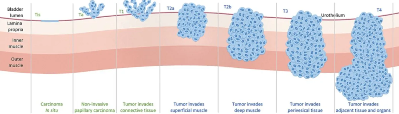
Fig. 1. Staging of bladder cancer

Tis or Ta tumors are considered non-invasive, whereas tumors reached LP and beyond are considered invasive. (From https://www.anchiano.com/clinical-features/)

Base on the depth and location of the tumor, bladder cancer can be characterized into different stages [5]. The deeper tumor grows the more severe the disease progresses. The diagram above shows the staging of bladder cancer defined by the TNM classification (Tis-T4). Starting from the top, the Tis is a flat non-papillary lesion. The Ta stage indicates all observed tumors are non-invasive with papillary architecture. The papillary tumor is described as the shape which looks like corals under the scope. Although it often grows outward into the bladder lumen, it is not guaranteed that it will not also grow inward into the submucosal layer. The T1 represents at least one observed tumor that has invaded into the subepithelial connective tissue. At this point, this type of tumor is considered invasive. Finally, T2, T3, and T4 tumors represent the tumor that has reached or penetrated through the muscle layer. These tumors are considered muscle-invasive bladder cancer [5]. Based on the staging and characterization reported by pathologists, the patients will receive different treatments. In a nutshell, accurate staging is important as different management strategies are often employed for non-invasive versus invasive or non-muscle-invasive versus muscle-invasive bladder cancers [2,4,5].

(9)

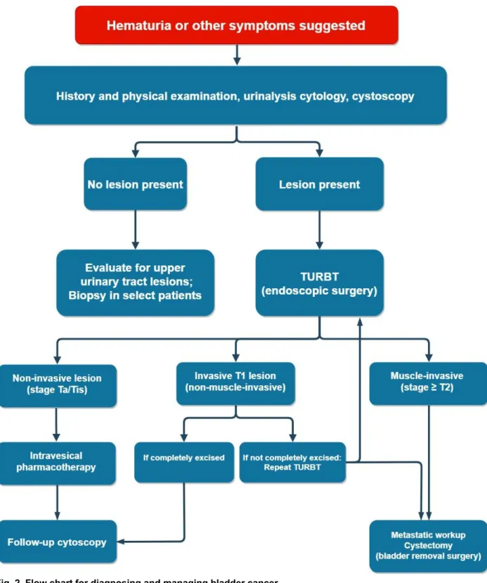
Fig. 2. Flow chart for diagnosing and managing bladder cancer.

The patients go through a series of examinations before performing any invasive treatments. The management options are determined after the histopathological characterization of the tumor.

(10)

Clinical management of bladder cancer

The treatment of a bladder cancer patient is not determined by just one doctor but a series of confirmation and discussion from a team of specialists [6]. In the clinic, there are standard operational protocols in examining possible bladder cancer cases. A surgeon would need to confirm multiple signs of bladder cancer such as hematuria and cytokine profile in the urine before performing any invasive treatments to a patient [7]. Thus, almost all of the specimens that pathologists receive from the surgeons/urologists are likely pieces of tissue specimens from transurethral resection of bladder tumor (TURBT) [6,7]. In other words, by the time of TURBT, the surgeons are very confident that there are growing tumors in the bladder. With that said, creating a machine learning system that is able to distinguish cancer tissue versus healthy tissue is not urgently needed in the medical field. Systems that emphasize on characterizing cancer type is much more in demand.

As outlined in the overall classification section, accurate diagnosis of non-invasive versus invasive bladder cancers is very important as they are often managed differently [5,6]. In particular, the staging system plays a critical role in predicting patient outcomes. If a patient is found to have T1 bladder cancer in the TURBT specimens, it does not guarantee that it will remain within the LP layer as a non-muscle invasive tumor. Moreover, in many cases, the tissues that are used in the pathological examination are fragmented without a muscle layer. In addition, it is often very difficult to confirm the T1 stage without the presence of the muscle layer in the specimen. After all, removing tumors under a cystoscope is not an easy task. The

surgeon cannot guarantee the tumors dug indeed contain the muscle layer of the bladder [5,8]. When this happens, the pathologist would either request the surgeon to perform another surgery for obtaining deeper samples or have to work further with what he/she has.

(11)

Pathological importance

A pathology report after reviewing a patient’s tissue sample often serves as the gold standard in the diagnosis of various diseases [9]. Especially in cancer diagnosis, the biopsy report from a pathologist plays a central role in determining the appropriate therapy for the patient. However, the reviewing of pathological slides is a very complex task, requiring years of training to gain the experience to do well. The pathologists need to evaluate patient’s tissue under the microscope with their naked eyes and occasionally by scoring biomarkers [10].

Screening through pathological slides is a very tiring job. Standardized, accurate and reproducible pathological diagnoses are essential keys to advancing precision medicine. Since the mid-19th century, the primary tool used by pathologists to make diagnoses has been the microscope. In order for a pathologist to make a good judgment, it takes years of practice, experience, and stamina [6,10,11]. Even with years of training, a discussion between peers for confirmation is necessary, which makes the whole process even more time-consuming. Over the past several decades there have been increasing interests in developing computational methods that relate to machine learning to assist images in pathology [12-16]. Ranging from screening breast tumor on X-ray pictures [14] to identifying/characterizing tumor cells in histology slides [12,13,16]. Developing a computer system to assist pathological diagnoses provide not only the possibility to ease the workloads from the pathologist but also new ways to merge different medical examination from a different department.

Pathological slides

Combining machine learning algorithm on pathological images has been ongoing for several years. From our literature search, we have found two major histopathological image inputs in the pathological analysis in machine learning: H&E staining and immunohistochemistry

(12)

(IHC) staining [13,16,17]. Although both types of staining applied directly onto the tissues from real patients, they served for very different purposes. The H&E staining is generally used for reviewing the histological structure of the specimen in which tissues are stained using a blue dye called hematoxylin and a red dye called eosin. The staining results in a spectrum of different color intensities from blue and violet to red due to different absorption of dyes. These morphological patterns are often enough for pathologists to characterize and predict various cancer statuses. The IHC staining, on the other hand, reveals the expression of a specific protein in tissues. Beside only hematoxylin staining for revealing tissue pattern, positive signals are from a brown color dye called biotin which only binds to the antibody that targets the protein of interests. Based on the intensity and the location of the protein, pathologists can accurately classify the disorder. However, compared with H&E staining, machine learning technology on IHC staining is less urgently needed in pathology practice. Because most cancers do not have well-defined biomarkers and no one knows which protein(s) should be stained [10], H&E staining is much universal and more widely used in pathology department around the world. This is also why having a new tool for recognizing H&E-stained slides is more translational than IHC-stained slides.

In the context of cancer characterization, a number of computational imaging

approaches have recently been applied to pathological slides. For example, cancer grading related phenotypes such as the ratio of cell size to nucleus size, circularity of the cell shape, color of cytosol, number of infiltrated lymphocytes per cancer cell, can now be quantified automatically by turning slides into digital files [15]. The correlation of quantitative histological features with molecular features reveals cancer aggressiveness [12,15]. These parameters were not only once considered impossible to collect through human’s naked eyes but also difficult to proceed to a complete statistical analysis [13,16]. With recent advancement in

(13)

imaging processing methods and machine learning analysis algorithms, they now provide new potentials for cancer characterization.

Computational approach

In the era of big data, scientists around the world have generated millions of data for disease characterization and recognition. As more and more data gets generated and uploaded, they have become almost impossible for the human brain to conceptualize. In the computer science community, many researchers have used machine learning approaches operate such high dimension data sets. By pairing the cases of normal tissue vs cancerous tissue, supervised machine learning methods such as logistic regression, naive Bayes nets, support vector machine (SVM), and random forest have been proved to provide accurate categorization when comparing to pathologists’ judgment [12,15,18]. When combining with other staining techniques to reveal oncogenic markers such as HER2 expression in breast cancer cells, computer with artificial neural network training is able to categorize the tumor subtype through digitizing the intensity of the marker [14]. Moreover, instead of just using cancer vs non-cancer as an

outcome, as many models did, researchers can even predict the lifespan of the patient solely on morphological patterns of cancer [10]. However, due to the inconsistent case number and funding in medical research, most promising projects that relate to machine learning largely focus on well-known diseases such as breast and lung cancers. In fact, less common diseases such as bladder cancer are rarely discussed and show little interests in machine learning.

(14)

Key morphological features for distinguishing non-invasive and invasive tumors

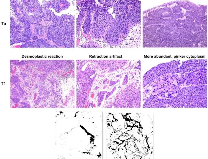
Pathologists often use three key microscopic patterns for distinguishing non-invasive versus invasive bladder tumors [19]. First, the desmoplastic reaction can be seen in a focus of invasive tumor surrounded by excess fibrous pink connective tissue and immunocytes (tiny cells with scant cytoplasm). Second, artificial retraction, due to dehydration during tissue processing, can be seen around the nest of tumor cells as spaces/cracks. Third, invasive tumor cells

occasionally show more abundant, pinker cytoplasm, compared with that of non-invasive tumor cells, possibly due to differences in the microenvironment such as pH value. In addition, the relative distance of the tumor nest to the muscle layer may predict tumor invasion. Regardless of the shape or color of the tumor, when a tumor is found growing within the muscle layer, it will be considered as the T2 stage. However, as we previously mentioned, if the surgeon did not dig deep enough into the muscle layer during TURBT, the pathologist might not be able to judge the case with this factor. Accordingly, alternative approaches for dealing especially with fragmented tissues are needed.

(15)

Fig. 3. The three key patterns for distinguishing non-invasive versus invasive bladder tumors

Representative images were selected for the purpose of demonstration. Retraction artifact exhibits crack-like shape around tumor nests.

(16)

Project foundation

In the world of data science, larger data size normally results in better performance. With a large number of data points, outliers are easier to classify and the underlying distribution of that data is clearer [20]. Unlike human limitation in conceptualizing high-dimensional data points, deep learning is able to digest and utilize a huge amount of information with unlimited dimensions. As most publications have suggested, modern deep learning models are able to outcompete human specialists by providing a bigger scope from big data [20]. However, not all disease are created equally. Uncommon scenarios and human errors can happen in some cases and may cause lots of confusion to the pathologists. Human-caused variation such as inconsistent histological staining and incomplete biopsies can be problematic even to an

experienced pathologist. As data size is becoming a prerequisite in using deep learning models, the machine learning development in the medical field also reflects the tendency by focusing on machine learning development on diseases with existing big data sets. As a result, diseases with relatively less complete data set, such as bladder cancer, are often neglected.

Although there has been a well-established system, it is occasionally difficult for pathologists to adequately characterize bladder cancers and have been concerning them for many decades. When characterizing a bladder biopsy, grading and staging are not always correlated with each other. The high-grade tumor can be found at an early stage disease. An aggressive tumor can be marked as Ta stage at the time of the surgery, but it does not guarantee to remain within LP.

Making an adequate histopathological assessment can sometimes be very challenging. The pathologists may receive low-quality specimens when the surgeon missed the crucial spots or simply did not dig deep enough into the muscle layer [5,21]. Since the whole structure of the tissue serves as an essential reference for pathologists’ judgments, fragmented tissue makes

(17)

characterization a lot harder. If the case is too ambiguous to judge, pathologists would use the favoring system to merge thoughts with other pathologists. By giving stars that represent the likelihood of the cancer type and sum up the votes from multiple pathologists, a final judgment will be made. In such cases, the number of stars is considered as the most objective numeric value. As pattern recognition in data science is becoming more and more mature, new machine learning models that look for patterns even in fragmented tissues can greatly help pathologists by providing extra values in the flavoring system.

In the clinical practice, according to the pathologists in the University of Rochester Medical Center (URMC), surgeons and pathologists have been fascinating in finding alternative ways to distinguish non-invasive and invasive bladder cancer cases. Importantly, there is little difference in treating T1 non-muscle invasive versus T2~T4 muscle-invasive bladder cancers, whereas Ta/Tis tumors are treated very differently from T1~T4 invasive diseases. Therefore, the essence of this research does not aim to replace pathologists by out beating human judgment in performance. Instead, we are trying to make a model that collectively recognizes the features of bladder cancer invasion in histological images. It can then help pathologists to make a better judgment when facing ambiguous cases.

(18)

Results

H&E staining quality and image processing

In order to find real pathological slide images as training and testing sets, we used real histopathological slides from the archives at URMC. All these slides stained with H&E were used for issuing pathological reports. To digitize these slides, all raw images were captured at X100 magnification with 2,048 by 2,048 pixels. Although the overall image from the camera is very clear, a dark spot was found at the lower right-hand corner. Therefore, to target regions with pathological changes, we cropped and tiled the central part of the raw image to get smaller images of 700 by 700 pixels. In total, we obtained 1,177 H&E stained histopathology images. To keep the training cases as real as possible, all bladder tumors in the study were restricted within Ta/Tis/T1 stages.

Quantitative representations of microscopic patterns

Graphical patterns were first translated into numeric values for computational approaches. In order to turn human knowledge based patterns into quantitative values, we used ImageJ and CellProfiler to extract image patterns into numbers. To extract objective morphological patterns of invasive tumors from thousands of images, we built 9 fully automated image pattern

extraction pipelines to collect 3 of the 4 key features suggested by the pathologists. Due to the complexity of pathological patterns, each pattern was a combination of various subpatterns. To capture as much information as possible, we used multiple numeric features to represent one cancerous pattern. After masking the unwanted area using methods like color thresholding and matrix subtractions, we are able to extract each pattern into various features. Since all of the raw images were from URMC slide archive and were consistent in quality, the parameters for extracting each feature were consistent across all images. The image features included nucleus

(19)

size distribution, crack edge, sample ratio, distribution of pixel intensity in the connective tissue and cytosol as well as the shape of connective tissue and nuclei. The quantitative features were outputted as spreadsheets in which the features were represented as a column and each pattern was represented from multiple features. Each pattern was measured separately and merged into a giant comma separated value (CSV) file where rows represent the image and columns as features from a variety of cancerous pattern. A total of 740 quantitative features were extracted from 1,177 bladder cancer images.

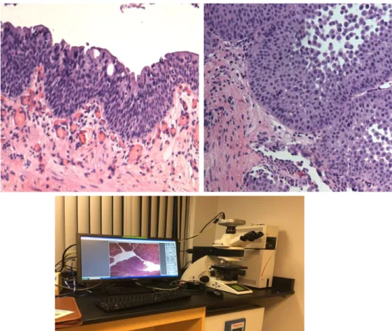
Fig. 4. Raw sample images from URMC slide archive

H&E slides were captured with 100-fold magnification under the microscope. The image was digitized by a digital camera attached on top of the microscope. The parameters for capturing the image were uniform through the digitization. Regardless of the identical setting on the hardware, the image still showed up a little different in the image. Post image processing for normalization was required.

(20)

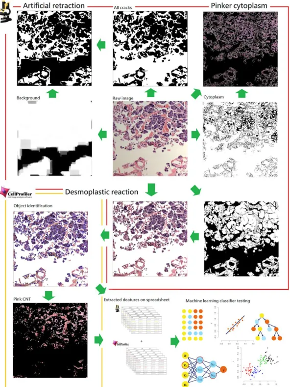
Fig. 5. Image processing methods for finding the features suggestive of tumor invasion in pathological images

Images were preprocessed before feature extraction. The artificial retraction and pinker cytoplasm were measured under ImageJ environment. The mask was created for blocking off the unwanted region and the pattern information was recorded. The desmoplastic reaction was extracted in CellProfiler environment. The image was first

preprocessed by masking off the non-tissue area in ImageJ. The tissue only region images were then inputted into CellProfiler for farther features extraction. The features were outputted as spreadsheet before input into machine learning classifiers.

(21)

Cluster analysis

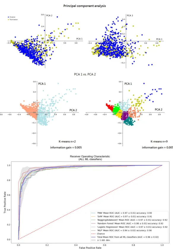
To test and understand the nature of the numeric values that represent the pathologists’ knowledge, we have done a simple cluster analysis for finding possible clusters from the data set. We first reduced data dimension through principal component analysis (PCA). Through PCA, we are able to rank top components by their eigenvalues. However, as Fig. 6a suggested, when plotting the top components with the highest eigenvalue, no visible clusters were found. In addition, by performing k-means analysis on PCA components, we found there were no pure clusters from k=2 to k= 9 (Fig. 6b). Combining principal component analysis with k-means, the non-invasive and invasive images were highly overlapped. Splitting the clusters resulted in less than 0.006 in information gain.

These data suggested that we are not able to separate the data with the simple linear transformation. Among the 696 features about the image, most of them might be noise. Dimension reduction and more sophisticated classifiers were needed for building the model.

(22)

Fig. 6. Quantitative image features for distinguishing invasive patterns.

The top 3 components from the principal component analysis were plotted and no distinguishable cluster was found. The ROC curves for classifying invasive bladder cancer cases from the URMC test set. Classifiers with all 696 features attained average AUC of 0.96. The performance of different classifiers is shown. ROC, receiver operator characteristics. AUC, the area under the curve.

(23)

Dimension reduction

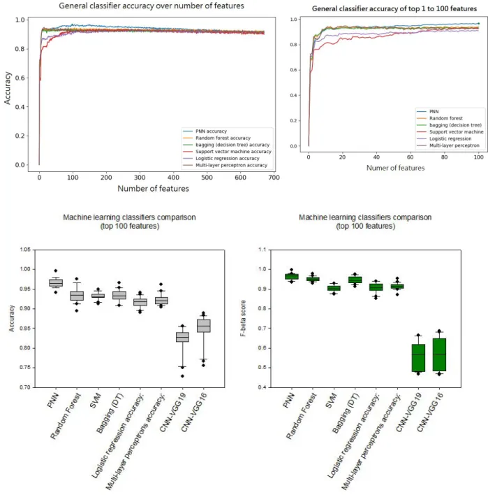
The uninformative parameters were trimmed off based on the nature of the data. There were 740 columns of features after merging features from ImageJ and CellProfilers. To exclude meaningless features, features related to time, index, string, and ‘NA’ were deleted from the dataset. In addition, numeric values that are less than 3 sets of number or increments by row number were also considered unusable. After excluding uninformative features, 696 features were left as possible indicators of invasive profile. As there were only around 930 images used as training sets in each round, using 696 features as the input was still considered too many for machine learning classifiers. To avoid overfitting, decision trees with k-fold cross-validation were used to rank the usefulness of each feature. We first used all 696 features as inputs to build 20 forests of 40 trees. Like the random forest, each tree was constructed by random samples, but the number of features was fixed as 696. As the model constantly evaluates the importance of each feature when a tree is generated, an average of each feature importance was generated from each forest. By accumulated the usage of each averaged feature from each forest, we were able to evaluate the relative importance of each feature. The resulting rank of the importance of the first model was used in the subsequent machine learning models. We measured the impact of the first feature and iteratively added the next feature in the rank. As shown in fig. 7a, as we increased the number of features in the order of ranking from bagging, the performance of classifiers such as a probabilistic neural network (PNN) also increased and reach max around 70 to 110 features. After 200 features, the performance started to drop until it overlapped with forest classifier around 400 features. From this approach, we not only found that more than half of the features extracted from the images were noises but also decided to focus on the top 100 features that were responsible for the performance for PNN.

(24)

Since the performance of PNN reached a plateau after 100 features, we further

evaluated the performance of 6 classic machine learning classifiers by using only 100 features as inputs. By taking the mean performance from all 6 classic machine learning classifiers, the overall performance of the top 100 features resulted in around 91.6% in accuracy. Also, like the previous approach suggested, PNN outperformed other classifiers with the area under the curve (AUC) of 0.99 and accuracy around 96.7%. Together with the overall feature numbers to

(25)

Fig. 7. Top quantitative features on machine learning classifier performances

The impact of the number of features on 6 classic machine learning performance was recorded. The features were inputted by the order of relative importance that ranked by multiple decision tree classifiers. The most significant improvement of performance was in the first 100 features. The best mean performance was at the top 100 features. The top 100 was used as the cut point for determining the features that are considered useful in the model. The accuracy and F-beta score(beta = 1) were used for comparing the performance among different machine learning classifiers.

(26)

General machine learning classifier comparison

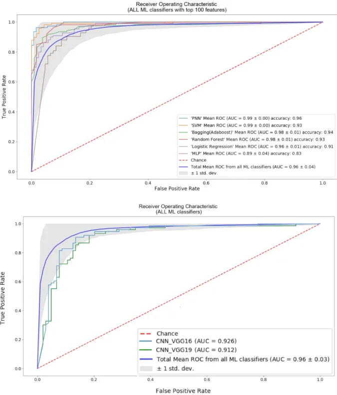
Even though the performance of human experience features with classical machine learning classifier was very good, we were also wondering if fully automated deep neural networks could outperform out our model as most publication suggested. Then, we decided to test the performance of computer-based features extraction from popular convolutional neural network (CNN) models directly on the raw images. To focus on testing the performance of feature extraction from deep learning, we tested the performance of two well-known CNN models. The VGG16 and VGG19 were used to represent CNN on distinguishing non-invasive and invasive bladder cancer images. We directly inputted the 700 by 700 pixel H&E images into the CNN models and tested the quantitative features from its hidden layers. Since the ratio of invasive over noninvasive cases in the training set and testing set always was set to 1:1, we used accuracy as the prior metric in the lost function. Moreover, to make the comparison consistent, we trained and tested the CNN with the same training and testing cases used on traditional machine learning classifier. In addition, to fairly compare the performance of

human-based knowledge, We took the average of true positive rate and false negative rate from 6 classical machine learning classifiers, Multilayer Perceptron (MLP), random forest, SVM, logistic regression, bagging, and PNN to represent the quality of human-aid quantitative features. The accuracy showed CNN with VGG16 or VGG19 as hidden layers only reached around 81% or 85% whereas the top 100 human aid quantitative features with general machine learning classifiers reached around 91% and can be peaked as high as 96% in PNN. When comparing the AUC from ROC, the CNN-VGG16 was 92.16% and 91.2%, whereas the quantitative features from the human experience was 96.3%. Finally, as these performance metrics suggested, under limited data set and with human-aid quantitative features, general

(27)

machine learning classifiers such as random forest, PNN, and logistic regression outperformed deep learning model CNN-VGG16 and CNN-VGG19 performance better than CNN that

(28)

Fig. 8. Quantitative image features from CNN and human-directed pipelines

Six general machine learning classifiers (all ML classifiers) were used to represent the quality and the potential of human knowledge based features. The CNN with VGG 16 and VGG19 as hidden layers was used to test the performance of CNN. The AUC from the blue line is the averaged performance from the 6 classic machine learning classifiers.

(29)

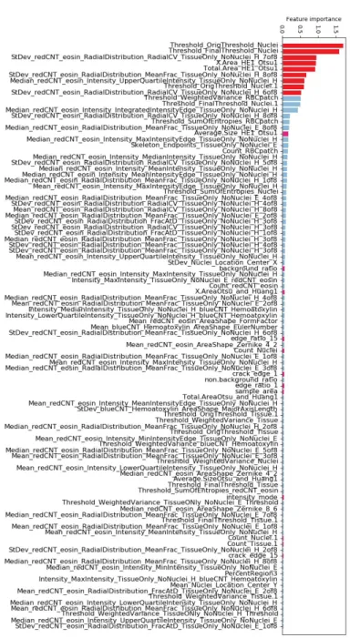
Fig. 9. Accumulated feature importance from bagged decision trees

The top 100 importance values are sorted from the highest to the lowest. The importance of a feature is computed as the (normalized) total reduction of the criterion brought by that feature. The top 9 features were related to nucleus

(30)

Pattern importance and newly discovered features

To further quantify the relative importance of the 3 key patterns suggestive of invasive bladder cancer, we approached it by separately testing the patterns of artificial retraction and eosin intensity in the cytoplasm. By doing so, it enables us not only to reveal which pattern is relatively more important than the other but also to dig deeper into the patterns. After testing the performance of multiple machine learning classifiers by input different features, we found the desmoplastic reaction was the most important pattern among the three. The top 90 features from the desmoplastic reaction averaged 92% in accuracy, whereas the artificial retraction and pinker cytoplasm averaged around 73.0% and 73.8%, respectively, (Figure 9). However, when looking deeper into the top 100 features from all features, all of the features from the

desmoplastic reaction, artificial retraction and, pinker cytoplasm, we found that the features that were heavily reused were mostly from desmoplastic reaction(Figure 10).

Unlike most deep learning methods that find data features automatically, using traditional machine learning classifiers on image recognition relies heavily on the quality of human-directed feature extraction. Extracted features that fairly represent the pattern of interest are

time-consuming and require lots of testing. However, one of the merits of using human experience-based feature extraction was the ability to understand the meaning of quantitative features. Unlike most deep neural networks that worked like a black box, we were able to open the classifiers, to evaluate the features and to learn which patterns were more important than the other. To investigate which features served as better indicators in representing cancerous patterns, we dug into the top 100 features evaluated by 40 decision trees. As shown in Fig. 9, almost all of the top features were related to the pattern of desmoplastic reaction. This

(31)

differences in the tumor microenvironment between non-invasive and invasive bladder cancers. Among the 3 key patterns, the desmoplastic reaction plays the most important role in

determining tumor invasion. In addition, when looking deeper into the top feature that represents desmoplastic reaction, features such as the number of nuclei and distributions of nuclei sizes came out at the very top in our ranking. These features seemed to be straightforward but were almost impossible for pathologists to actually calculate in their daily practice. Only with

(32)

.

Fig. 10. Accumulated feature importance from bagged decision trees

The top 100 importance values are sorted from the highest to the lowest. The importance of a feature is computed as the (normalized) total reduction of the criterion brought by that feature. The top 9 features were related to nucleus sizes

(33)

Material and Methods

Histology slides:

Through the generosity of Dr. Miyamoto, the digitized H&E bladder cancer images were collected from the Pathology Department of URMC. All H&E stained histopathological slides were obtained from real patient tissues. All tumor specimens were gathered by surgical excision (TURBT) and processed following the standardized protocol at URMC. In a total of 1,177

images were used for constructing the models, which included 460 non-invasive and 717 invasive cases. The label of images served as ground truth. To keep the training cases as real as possible, all images were from Ta, Tis, or T1 tumors. Muscle-invasive cases (T2 stage and above) were excluded from the analysis.

Image digitize system:

To digitize pathological slides, a Leica upright microscope DM5000 B research

microscope attached with a high-resolution camera from MacroFire was used for capturing the raw H&E staining images. The camera was able to capture a field of 2,048 x 2,048 pixels under 100X magnification. Image files were saved as tiff format. The central part of the raw images with 100X magnification was tiled into 700 X 700 pixels using the ImageJ based script with crop function in ImageJ. All images were cropped at the sample dimension.

Image processing system:

Due to the fact that CellProfiler demands stable image quality, the raw images were first cropped into 700X700 pixels. Then, copies of the cropped images were standardized by

pre-processed with the FFT function from ImageJ if needed. The function evened the light intensity by normalizing the darkest corner to the brightest corner on the image. These

(34)

pre-processed-cropped images were then processed into black and white pictures for masking the region of disinterests. The images containing only lesions of interest were sent into the CellProfiler for further analysis.

Image feature extraction:

The feature extraction was performed using CellProfiler and ImageJ. Both packages enabled us to create and customized pipelines for extracting various patterns about the image. ImageJ provided a scripting interface by using its own scripting language called MacroJ. It enabled us to extract patterns that had not been published before. The invasive patterns of artificial retraction, nucleus size, and the cytosol color were extracted by ImageJ. The pattern of connective tissue around the tumor and all nucleus shape pattern in the image were extracted by using CellProfiler. CellProfiler provided multiple built-in cellular features extracting modules. For every image, 60 different features were extracted by ImageJ and 636 features were extracted by CellProfilers. Overall, ImageJ enabled us to extract features that represent the whole tissue. CellProfiler focused on extracting features of an individual cell. The spreadsheets generated from ImageJ and CellProfiler were merged into a data frame in R environment. The Macro scripts from ImageJ and the pipeline file from CellProfiler were provided. [GitHubLink] ImageJ[https://imagej.nih.gov/ij/]. CellProfiler[http://cellprofiler.org/]

Statistical analysis and plotting

All statistical analyses in the project were performed under the R environment [22]. To set the bin size for color spectrums, the total image pixels were processed and evaluated through r programming. The performance metrics including accuracy, ROC, AUC, and F-beta score were calculated by using functions from Scikit-Learn metrics. The plots for representing

(35)

ROC curves and AUC score of all machine learning models were generated by using python package: matplotlib. The boxplots for representing the performance of all machine learning models were generated by SigmaPlot ver.12.5.

Data processing packages

Since most numeric features were extracted from different image processing tools, different data processing packages were used. All results were saved as CSV format. To

combine all of the CSV files, a small script was written in R to confirm the proper merging and to output a bigger spreadsheet. Pandas were used for data processing and subsetting. The big CSV file was transformed into Numpy matrix before putting into machine learning models.

General machine learning models

The general machine learning classifiers in the project were all from well-known python packages. The probabilistic neural network framework was from Neupy package. All of the ensemble learning models, including SVM, logistic regression, decision tree, random forest, and multilayer perceptron, were from Scikit Learn package. The datasets were randomly partitioned into 70% training set and 30% testing set for every testing. To ensure the robustness of the results, the random partitioning process was repeated 20 times and a mean of 20 performances was used to represent the overall performance of the classifier.

Artificial neural networks

There were three different artificial neural network models used in this project: MLP, PNN [23-26], and CNN. The MLP was constructed by using packages from Scikit-Learn. It is a simple deep neural network with two hidden layers composed of 16 and 23 neurons and ‘tanh’ as the

(36)

activation function. The PNN was a pre-made model from Neupy. The convolutional neural network was constructed by using Keras. The ImageDataGenerator from Keras was used for imaging processor. Three pre-trained hidden layers for image feature extraction were used from VGG16 and VGG19.

Discussion

For the four main morphological patterns of invasive bladder cancer, suggested by

pathologists, we have successfully designed and extract 696 features that represent 3 of the 4 invasive patterns: desmoplastic reaction, artificial retraction, and pinker cytoplasm. We obtained them by processing images using ImageJ and CellProfiler. We did not extract the pattern of muscle layer because of two fundamental reasons. First, the muscle layer is very easy to be recognized by the naked eye. Whenever there is a tumor invading the muscle layer, the tumor is not only considered as an invasive type but also staged as T2 muscle-invasive tumor. Second, one of the biggest problems that pathologists are facing is the incomplete assessment of tissue. This indicates that the muscle layer is often missing from the tissue. Thus, one of the biggest aims of the project is to construct a recognition model that is able to classify tumor type in fragmented bladder biopsy specimens without the muscle layer. As our model reached a good performance in distinguishing non-invasive versus invasive images with above 90% in accuracy, the invasive tumor might have to reconstruct the microenvironment within the muscle layer before invading into it. By digging deeper into these invasive patterns, we may get a better understanding of the mechanism of bladder cancer in building the precancerous

micro-environment.

Unrelated cancerous patterns on pathological images may represent some correlation with each other. When introducing only the features that represent artificial retraction and

(37)

pinker cytoplasm into the classical machine learning classifiers, the models were able to achieve around 85% in accuracy. Although the accuracy was not as high as just using

desmoplastic reaction features that reached above 90%, the result also indicates that most of the images have multiple invasive patterns. In other words, most artificial retraction and pinker cytoplasm images appeared in the desmoplastic reaction environment. The pattern of

desmoplastic reaction might affect that of an artificial retraction or there was a positive strong correlation between the two patterns. Once again extensive research is necessary for solving the puzzle.

Conclusion

Using CNN on medical image recognition is indeed becoming more and more popular. With enough data size, it consistently outperformed traditional machine learning models. But when the case number is limited, deep learning models may not be able to find the crucial features, resulting in a bias. Therefore, when facing limited data cases like recognizing tumor invasion in inadequate tissues, using human knowledge with general classifiers would be a great alternative approach. General machine learning models can be a powerful tool in helping pathologists diagnosing diseases. By collectively analyzing and sorting the known patterns, it can help not only the pathologists to stage and characterize bladder tumors by providing exceptional precision ranking but also medical science to evaluate which pattern or feature is more important than the others. Despite their wide application in medical diagnosis, they should not be considered as the final tool for decision making of the condition for the pathologists who are responsible for final interpretation of the output of the models.

The neural network-based clinical support systems provide the medical experts with second opinions about the pathological patterns. When facing specimens without the presence

(38)

of muscle layer, machine-based image categorizes system can give a risk or confident value to help pathologists making reasonable judgments. In this way, surgeons would improve the patient’s experiences of treatment by reducing the necessity of repeating TURBT on patients[5,6].

Future Work

There are several interesting approaches that can be extended from this project. First, the pipeline for image processing and the features extraction can be reconstructed into the plugins for ImageJ. Our current approach is using the MacroJ script with tested parameters to fetch invasive patterns about the image. The biggest reason we established our own image feature quantitative methods is that there were no ImageJ plugins that could provide the same approach. Since ImageJ is written in Java and the ImageJ community has released a Java library for constructing ImageJ GUI plugin, we can build a new GUI plugin by translating the ImageJ script into Java. This way, researchers without coding experience can also extract cancerous features from H&E images. Second, we did not test the full potential through testing on all of the parameters that Scikit-learn provided. Through testing different mathematical formats, we should be able to learn more about the features of invasive bladder cancer cells. Third, testing different pre-trained CNN models with more labeled images. Due to the limited image number, the performance CNN was greatly handicapped. As URMC pathology

department has archived over 10 years of patient slides, passing the requirement for CNN data size is not impossible. With the larger amount of data through repeating digitize pathological slides in URMC, we could make a more well-rounded characterizing system based on different pre-trained CNN models such as VGG, U-Net, ResNet, and GoogLeNet. We believe that with enough sample, using different CNN networks would extract a wider range of features that have

(39)

not yet been discovered and would ultimately helpful in distinguishing cancer types. Lastly, introducing active learning by interactively querying the user to obtain the desired outputs at new data[22, 23]. As there are known features highly indicative of tumor invasion recognized by pathologists, it will be interesting to merge these with image features that are collected by ResNet or VGG before putting them into the classifier. We can construct a deep neural network by combining human experience and computer knowledge to make the model less like a black box. This likely provides a more explainable output to the doctors.

References

1. Bray F, Ferlay J, Soerjomataram I, Siegel RL, Torre LA, Jemal A, Global cancer statistics 2018: GLOBOCAN 2018. CA: A Cancer Journal for Clinicians 2018;0:1_-31.

2. Knowles MA, Hurst CD. Molecular biology of bladder cancer: new insights into pathogenesis and clinical diversity. Nature reviews cancer. 2015;15:25-41.

3. Frampton JE, Plosker GL. Hexyl aminolevulinate in the detection of bladder cancer: profile report. BioDrugs clinical immunotherapeutics, biopharmaceuticals and gene therapy.

2006;20:317-20.

4. Stein JP, Lieskovsky G, Cote R, Groshen S, Feng A-C, Boyd S, et al. Radical cystectomy in the treatment of invasive bladder cancer: long-term results in 1,054 patients. Journal of clinical oncology. 2001;19:666-75.

5. Babjuk M, Oosterlinck W, Sylvester R. European Association of Urology guidelines on non-muscle invasive bladder cancer (TaT1 and CIS). Arnhem: European Association of Urology. 2012.

6. Sharma S, Ksheersagar P, Sharma P. Diagnosis and treatment of bladder cancer. American family physician. 2009;80:717-23.

(40)

7. Chang SS, Bochner BH, Chou R, Dreicer R, Kamat AM, Lerner SP, et al. Treatment of non-metastatic muscle-invasive bladder cancer: AUA/ASCO/ASTRO/SUO guideline. The journal of urology. 2017;198:552-9.

8. Stenzl A, Cowan N, De Santis M, Jaske G, Kuczyk M, Merseburger A, et al. European Association of Urology guidelines on bladder cancer, muscle-invasive and metastatic. Update March. 2008.

9. Leong AS, Zhuang Z. The changing role of pathology in breast cancer diagnosis and treatment. Pathobiology: journal of immunopathology, molecular and cellular biology. 2011;78:99-114.

10. Kumar V, Abbas AK, Fausto N, Aster JC. Robbins and Cotran pathologic basis of disease, professional edition e-book: Elsevier health sciences; 2014.

11. Oberman HA. Rudolph VIRCHOW: pathologist, anthropologist and statesman. Oral surgery, oral medicine, and oral pathology. 1961;14:975-80.

12. Cruz-Roa A, Gilmore H, Basavanhally A, Feldman M, Ganesan S, Shih NNC, et al. Accurate and reproducible invasive breast cancer detection in whole-slide images: A Deep Learning approach for quantifying tumor extent. Scientific reports. 2017;7:46450.

13. Wang D, Khosla A, Gargeya R, Irshad H, Beck A. Deep Learning for Identifying Metastatic Breast Cancer 2016.

14. Geras KJ, Wolfson S, Shen Y, Kim S, Moy L, Cho K. High-resolution breast cancer screening with multi-view deep convolutional neural networks. arXiv preprint arXiv:170307047. 2017.

15. Yu KH, Zhang C, Berry GJ, Altman RB, Re C, Rubin DL, et al. Predicting non-small cell lung cancer prognosis by fully automated microscopic pathology image features. Nature communications. 2016;7:12474.

(41)

16. Vandenberghe ME, Scott ML, Scorer PW, Soderberg M, Balcerzak D, Barker C. Relevance of deep learning to facilitate the diagnosis of HER2 status in breast cancer. Scientific reports. 2017;7:45938.

17. Cook HC. Origins of ... tinctorial methods in histology. Journal of clinical pathology. 1997;50:716-20.

18. Spanhol FA, Oliveira LS, Petitjean C, Heutte L. A Dataset for Breast Cancer Histopathological Image Classification. IEEE transactions on bio-medical engineering. 2016;63:1455-62.

19. Wallmeroth A, Wagner U, Moch H, Gasser TC, Sauter G, Mihatsch MJ. Patterns of metastasis in muscle-invasive bladder cancer (pT2–4): an autopsy study on 367 patients. Urologia Internationalis. 1999;62:69-75.

20. Yu S, Guo S. Big data concepts, theories, and applications: Springer; 2016. 21. Witjes JA, Redorta JP, Jacqmin D, Sofras F, Malmström P-U, Riedl C, et al.

Hexaminolevulinate-guided fluorescence cystoscopy in the diagnosis and follow-up of patients with non–muscle-invasive bladder cancer: review of the evidence and recommendations. European Urology. 2010;57:607-14.

22. Settles, Burr (2010). "Active Learning Literature Survey" (PDF). Computer Sciences Technical Report 1648. University of Wisconsin–Madison. Retrieved 2014-11-18.

23. Das, Shubhomoy; Wong, Weng-Keen; Dietterich, Thomas; Fern, Alan; Emmott, Andrew (2016). "Incorporating Expert Feedback into Active Anomaly Discovery". In Bonchi, Francesco; Domingo-Ferrer, Josep; Baeza-Yates, Ricardo; Zhou, Zhi-Hua; Wu, Xindong (eds.). IEEE 16th International Conference on Data Mining. IEEE. 853–858