CEED IN G S 27 . W OR KSH OP COM PU TA TION A L I N TE LL IG EN CE Herausgeber
F. HOFFMANN
E. HÜLLERMEIER
R. MIKUT
Dortmund | 23. – 24. November 2017
PROCEEDINGS 27. WORKSHOP
COMPUTATIONAL INTELLIGENCE
Dortmund | 23. – 24. November 2017
Dortmund | 23. – 24. November 2017
F. Hoffmann, E. Hüllermeier, R. Mikut (Hrsg.)
Proceedings. 27. Workshop Computational Intelligence
PRoCEEDINgs
27. Workshop
CoMPutatIoNal INtEllIgENCE
Dortmund, 23. – 24. November 2017
Herausgegeben von
F. Hoffmann
E. Hüllermeier
R. Mikut
Print on Demand 2017 – Gedruckt auf FSC-zertifiziertem Papier ISBN 978-3-7315-0726-0
This document – excluding the cover, pictures and graphs – is licensed under a Creative Commons Attribution-Share Alike 4.0 International License (CC BY-SA 4.0): https://creativecommons.org/licenses/by-sa/4.0/deed.en The cover page is licensed under a Creative Commons
Attribution-No Derivatives 4.0 International License (CC BY-ND 4.0): https://creativecommons.org/licenses/by-nd/4.0/deed.en Impressum
Karlsruher Institut für Technologie (KIT) KIT Scientific Publishing
Straße am Forum 2 D-76131 Karlsruhe
KIT Scientific Publishing is a registered trademark of Karlsruhe Institute of Technology.
Reprint using the book cover is not allowed. www.ksp.kit.edu
Inhaltsverzeichnis
V. Melnikov, E. Hüllermeier 1
(Paderborn University)
Optimizing the Structure of Nested Dichotomies: A Comparison of Two Heuristics
N. Ludwig, S. Waczowicz, R. Mikut, V. Hagenmeyer 13
(Karlsruhe Institute of Technology)
Mining Flexibility Patterns in Energy Time Series from Indus-trial Processes
T. Nguyen, J. Spehr, J.-O. Perschewski, F. Engel, S. Zug,
R. Kruse 33
(Volkswagen AG, Otto-von-Guericke Universität Magdeburg) Zuverlässigkeitsbasierte Fusion von Fahrstreifeninformationen für Fahrerassistenzfunktionen
C. Dengler, B. Lohmann 51
(TU München)
Actor-Critic Reinforcement-Learning in der Anwendung am Beispiel einer schweren Kette
M. Thill, W. Konen, T. Bäck 67
(TH Köln – University of Applied Sciences, Leiden University) Discrete Wavelet Transforms and Multivariate Gaussian Distri-butions for Anomaly Detection in Time Series
T. Münker, O. Nelles 73
(Universität Siegen)
Algorithms for the Identification of Merged Local Model Net-works
C. Klüver, B. Zurmaar 89
(Universität Duisburg-Essen)
Einsatz eines Self-Enforcing Networks zur kontrollierten Modell-bildung am Beispiel der Bewertung von Lösungen für Mathe-matikaufgaben
T. A. Runkler, J. M. Keller 103
(Siemens AG, University of Missouri–Columbia)
Sequential Possibilistic One–Means Clustering With Variable Eta
M. Gringard, A. Kroll 117
(Universität Kassel)
Zum Optimalen Offline Testsignalentwurf für die Identifikation dynamischer TS-Modelle: Multistufensignale für unsicherheits-minimierte Konklusionsparameter
H. Schulte, E. Gauterin 139
(Hochschule für Technik und Wirtschaft Berlin)
Optimierung von Entwurfsparametern für Takagi-Sugeno Fuzzy Sliding-Mode Beobachter mit Simulated-Annealing Verfahren
M. Wever, F. Mohr, E. Hüllermeier 149
(Paderborn University)
Automatic Machine Learning: Hierarchical Planning Versus Evolutionary Optimization
A. Cavaterra, S. Lambeck 167
(Hochschule Fulda)
Untersuchungen zur Verwendung von Takagi-Sugeno Fuzzy Sys-temen in modellprädiktiven Dual-Mode-Reglern
T. Loose, Th. Pospiech 175
(Hochschule Heilbronn)
Benchmark-Untersuchung zur Regelung schwach gedämpfter Systeme bei industriepraktischen Anwendungen
J. Stork, M. Zaefferer, A. Fischbach, T. Bartz-Beielstein,
F. Rehbach 195
(TH Köln)
T. O. Heinz, J. Belz, O. Nelles 211
(Universität Siegen)
Design of Experiments – Combining Linear and Nonlinear Inputs A. Bartschat, J. Stegmaier, S. Allgeier, S. Bohn, O. Stachs,
B. Köhler, R. Mikut 227
(Karlsruhe Institute of Technology, University of Rostock) Augmentations of the Bag of Visual Words Approach for Real-Time Fuzzy and Partial Image Classification
S.Bagheri, W.Konen, T.Bäck 243
(TH Köln, Leiden University)
Comparing Kriging and Radial Basis Function Surrogates
M.A. Rebolledo, O.M. Baez, T. Bartz-Beielstein, L. Ribbe 261
(TH Köln)
Bias-Correction of Satellite Rainfall Estimates Through the Use of Metamodels using Gaussian Process and Bayesian Regression. A Case Study for the Imperial Basin (Chile)
C. Holst, U. Mönks, V. Lohweg 279
(inIT, coverno GmbH)
Optimizing the Structure of Nested
Dichotomies: A Comparison of Two Heuristics
Vitalik Melnikov
1, Eyke Hüllermeier
2 Department of Computer SciencePaderborn University, Germany E-Mail: 1[email protected],2[email protected]
Abstract
In machine learning, nested dichotomies are used to decompose a multi-class multi-classification problem into a set of binary problems. The performance of a nested dichotomy strongly depends on the structure of such a decomposition. In this paper, we compare the random-pair heuristic, a state-of-the-art approach for optimizing the structure, with an extremely simple alternative: Leveraging a procedure for uniform sampling of dichotomies, the Best-of-K heuristic picks the (presumably) best among 𝐾randomly generated dichotomies. Interestingly, Best-of-K turns out to be highly competitive, and outperforms the random-pair heuristic in the case of simple base learners such as logistic regression.
1 Introduction
Nested dichotomies are known as models for polychotomous data in statistics and used as classifiers for multi-class problems in machine learning [4]. Based on a recursive binary partitioning of the set of classes, nested dichotomies reduce the original multi-class problem to a set of binary problems, for which any (probabilistic) binary classifier can be used. For example, the dichotomy shown in Fig. 1 decomposes a problem with four classes into three binary problems: The first classifier (𝐶1) is supposed to separate class 3 from the meta-class{1,2,4}, i.e., the union
of classes 1, 2, and 4; likewise, the second classifier separates classes
{2,4}from 1, and the third classifier the classes 2 and 4.
Once the hierarchy of classifiers required by a nested dichotomy have been trained, a new instance𝑥can be classified in a straightforward way,
C
1C
2C
31
2
3
4
Figure 1: Example of a nested dochotomy.
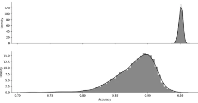
namely by submitting𝑥to the root of the dichotomy and propagating it to one of the leaf nodes, based on the decisions of the classifiers along the corresponding path. As an appealing property, we note that nested dichotomies allow for producing probability estimates (instead of hard class assignments) in a very natural way, provided each classifier predicts suitable conditional class probabilities at the inner nodes. In that case, the probability of any class𝑦is simply given by the product of conditional probabilities on the path from the root to the leaf node marked with𝑦. In practice, nested dichotomies have been shown to yield superb predictive accuracy [4, 6, 8]. Yet, the performance of the multi-class classifier even-tually produced may strongly depend on the structure of the dichotomy. In fact, the structure of a dichotomy specifies the subset of all binary problems that need to be solved, and some of them might be much more difficult than others. This is illustrated in Fig. 2, where the distribution of predictive accuracies (on the test data) of nested dichotomies is shown for the pendigits dataset. As can be seen, the variance is higher if logistic regression is used as a base learner, and smaller with decision trees. This observation can be explained by the fact that the latter is much more flexible than the former: A decision tree is a complex, highly nonlinear model, which can compensate a suboptimal structure much better than a simple linear model as fit by logistic regression (but of course also comes with a higher danger of poor generalization due to overfitting); or, stated differently, the choice of a suitable structure is much more critical when using simple models such as linear discriminants.
Consequently, finding a suitable structure is an important prerequisite for successful learning with nested dichotomies. Since the number of candidate structures is huge (double factorial in the number of classes),
Figure 2: Gaussian kernel density estimation of accuracy distribution for the pendigits dataset based on a random sample of 10000 nested dichotomies, using decision tree (CART, in the top plot) and logistic regression (in the bottom plot) as base learner.
several heuristic methods have been proposed for constructing dichotomies specifically tailored for the data at hand [2, 6, 3]. Although some heuristics are designed to select an optimal subset of nested dichotomies, to be
used as an ensemble of classifiers, we focus on finding asingle dichotomy
in this paper (for example because an ensemble is not desirable, due to reasons of complexity or interpretability).
According to recent empirical studies, the current state of the art is therandom-pair selection heuristic (RPND) proposed by Leathart et al.
[6]. At each inner node of a nested dichotomy, this approach obtains a split of the classes𝒴 associated with that node into two meta-classes
as follows: Two classes𝑌𝑖, 𝑌𝑗 ∈ 𝒴 are selected (uniformly) at random,
and the base learner is used to train a classifier𝐶𝑖,𝑗 discriminating these two classes. Both classes define the seed for a meta-class 𝒴𝑖 and 𝒴𝑗, respectively, and each remaining class𝑌 ∈ 𝒴 ∖ {𝑌𝑖, 𝑌𝑗}is added to one of these meta-classes, depending on whether𝐶𝑖,𝑗 assigns the majority of instances of𝑌 to𝒴𝑖or𝒴𝑗. Once the complete structure of the dichotomy has been determined, the classifiers at the inner nodes are trained on the corresponding splits.
In this paper, we reconsider the random-pair heuristic, challenging it with the arguably most simple heuristic one may image: generating𝐾 dichotomies at random and selecting the (presumably) best one. In Section 4, we demonstrate that this simple Best-of-K heuristic is highly competitive and, depending on the value 𝐾, even able to outperform the random-pair heuristic. As a side product, the paper makes another
interesting contribution, namely an efficient algorithm for sampling nested dichotomies uniformly at random. Although sampling procedures have already been used in several papers [4, 6, 2], an explicit algorithm has never been provided; interestingly, a naive sampling procedure will yield a non-uniform distribution.
2 Uniform random sampling of nested dichotomies
On the structural side, there is a one-to-one correspondence between nested dichotomies and binary trees. Since each node in a nested dicho-tomy has either none or exactly two children, every nested dichodicho-tomy is a (rooted) full binary tree. In addition, each leaf node in a nested dichotomy is labeled with the corresponding class. This labeling uniquely determines the dichotomies at all inner nodes. The problem of generating a nested dichotomy can therefore be divided into two steps: (i) generation of a rooted terminally labeled full binary tree and (ii) propagation of leaf labels towards the root in order to determine the dichotomies at the inner nodes.For the problem (i), several strategies were proposed in the literature [9, 5]. Here, we provide a two-step procedure for uniform random sampling of rooted terminally labeled full binary trees as suggested by Furnas [5]:
1. Generation of an unrooted terminally labeled full binary tree𝑇𝑐. Given is a set of𝑐 terminal nodes (leafs).
a) Create a doublet “tree”𝑇2 by connecting nodes 1 and 2 by a
single edge.
b) Until all𝑐 terminal nodes are connected to the tree, proceed with the following random augmentation:
i. Given a tree𝑇𝑘 on𝑘 < 𝑐terminal nodes, select an edge of𝑇𝑘 uniformly at random.
ii. On this edge, a new internal node of degree 3 is added and the (𝑘+ 1)st terminal node is connected. The result is a binary tree𝑇𝑘+1 on𝑘+ 1 terminal nodes.
2. Transformation of𝑇𝑐 into a rooted tree.
a) Choose an edge of𝑇𝑐 randomly with uniform probability. b) Introduce a new root node of degree 2 on this edge.
Furnas proved this procedure to provide a uniform random sampling of rooted terminally labeled full binary trees. The time complexity of the first step is linear in the number of classes𝑐. The second step can be implemented in constant time, leading to an overall time complexity of 𝑂(𝑐).
For the label propagation problem (ii), we suggest the following solution. Every leaf node is labeled with the number 𝑏𝑐𝑖 = 2𝑐𝑖, where 𝑐𝑖 is the corresponding class in the original problem. The dichotomies at the inner nodes are encoded with a pair of numbers [𝑑𝑙, 𝑑𝑟], denoting the sum of all leaf labels in the left and right subtree, respectively. Since all leaf nodes are encoded uniquely (with only a single ’1’ in the corresponding bit string), the dichotomy encodings are also unique. To propagate the leaf labels, we traverse the nested dichotomy in postorder and encode every inner node with the sum of the dichotomies of its child nodes [𝑑𝑙𝑙+𝑑𝑙𝑟, 𝑑𝑟𝑙+𝑑𝑟𝑟]. Since the complexity of tree traversal is linear in the number of nodes and the summation, and generating the leaf labels is nearly constant for a usual number of classes1, step (ii) has an overall
time complexity of𝑂(𝑐). Using this approach, a single nested dichotomy can be sampled uniformly with the time complexity𝑂(𝑐), i.e., linear in the number of classes in the original problem.
3 The Best-of-K Heuristic
Equipped with the sampling procedure for nested dichotomies from the previous section, the algorithm for the Best-of-K heuristic is quite straig-htforward. It is parametrized by the number𝐾 of nested dichotomies to be generated and evaluated. Given a (training) dataset with𝑐classes and a base learner, Best-of-K consists of three steps:
1. Sample 𝐾 nested dichotomies on 𝑐 terminal nodes uniformly at random.
2. Train these models on the given data with the provided base learner. 3. Select the best performing model based on the validation on the
training data (e.g., with the smallest training error).
1The length of the encoding number (as a bit string) is at most𝑐. Both encoding operations (bit shift and summation) will have roughly constant time for up to several hundred classes.
Several remarks on this approach are in order. First, since the sampling procedure only depends on the number of classes𝑐, and not on the data itself, it can be carried out in a preprocessing step, thereby reducing the overall execution time. Second, the training in the second step can be done independently for each nested dichotomy. Thus, Best-of-K is naturally implemented in a parallel way. If 𝐾 cores are available, a speedup factor close to𝐾 can be achieved in comparison to a standard (sequential) implementation (the runtime is the maximal training time of a single nested dichotomy). Third, while being computationally cheap, the selection of the best performing model based on the training error is arguably not optimal—a better selection could probably be made on the basis of a validation error. However, our experiments in the next section suggest this strategy to be good enough in general.
4 Empirical Study
We compare the Best-of-K heuristic with the state of the art RPND on 15 multi-class datasets (Table 1) from the UCI repository [1]. On every dataset, we perform the following evaluation: For a given parameter 𝐾∈ {1,5,10,20,50,100}, we generate a single nested dichotomy using
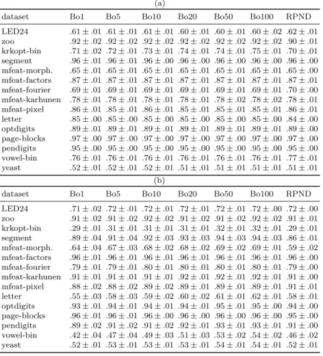
the Best-of-K heuristic and a single nested dichotomy using RPND. Both models are tested with two base learners: decision tree (CART) and logistic regression from the scikit-learn framework (ver. 0.19) [7]. The hyper-parameters of the base learners are set to default values, except for the minimal decrease of the impurity in CART, which is set to.0001 to prevent overfitting. Every generated nested dichotomy is trained multiple times by using 10-fold cross-validation, and the mean predictive accuracy is stored. Since both heuristics are randomized, we repeat this procedure 50 times for every dataset to stabilize the results. The mean and the standard deviation of predictive accuracy over these runs are given in the Table 2.
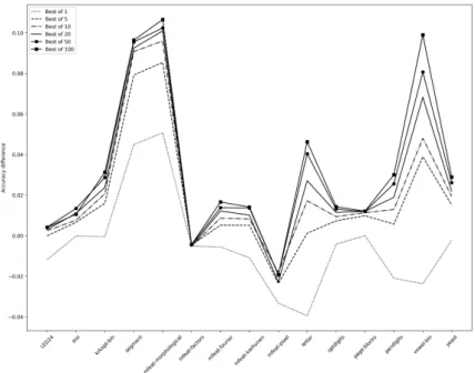
In Fig. 3, the difference𝐴𝑑𝑖𝑓 𝑓 =𝐴𝐵𝑜𝐾 −𝐴𝑅𝑃 𝑁 𝐷 in mean accuracy is shown. Unsurprisingly, the performance of Best-of-K increases for higher values of𝐾. For𝐾 >5, Best-of-K outperforms the RPND heuristic on most of the datasets if logistic regression is used as the base learner. For example, for𝐾= 5 and logistic regression as base learner, the mean time ratio over all datasets is 0.58 and the mean accuracy difference is 0.015. In the case of CART as a base learner, both heuristics perform comparable.
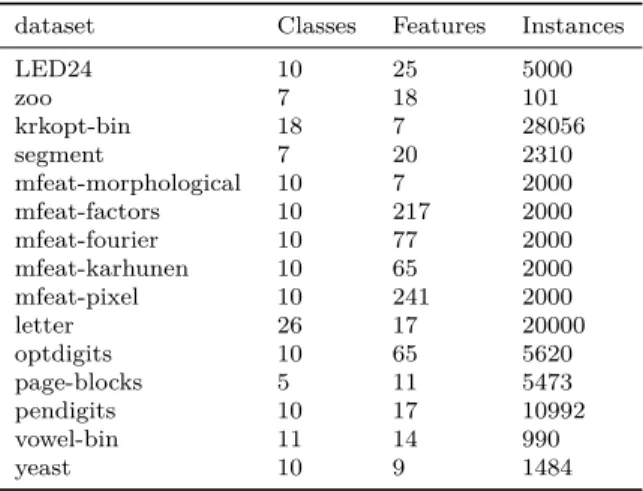
Table 1: The datasets used in the study. For the datasets krkopt and vowel, a one-hot encoding has been used for categorical features.
dataset Classes Features Instances
LED24 10 25 5000 zoo 7 18 101 krkopt-bin 18 7 28056 segment 7 20 2310 mfeat-morphological 10 7 2000 mfeat-factors 10 217 2000 mfeat-fourier 10 77 2000 mfeat-karhunen 10 65 2000 mfeat-pixel 10 241 2000 letter 26 17 20000 optdigits 10 65 5620 page-blocks 5 11 5473 pendigits 10 17 10992 vowel-bin 11 14 990 yeast 10 9 1484
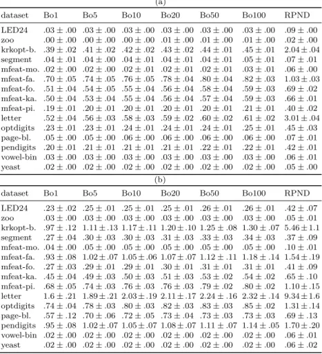
This seems plausible for the reason already mentioned: Since (unpruned) decision trees are able to generate complex models (with a tendency to overfit), they can compensate for a possibly suboptimal structure of a dichotomy. The small decrease in the performance of such models for higher values of𝐾suggests that, at least for some datasets, the selection of a nested dichotomy based on the training error is too optimistic. In Table 3, the mean and standard deviation of the generation time are given. The time was measured for the Best-of-K heuristic with parallelization, i.e., we assume to have𝐾 cores available and measure the maximal generation time for a single nested dichotomy. On a single core CPU, this heuristics would be roughly𝐾 times slower. The time comparison is provided in Fig. 4. The mean time ratio is defined as the ratio of mean times for generating a single nested dichotomy with both heuristics: 𝑇 =𝑇𝐵𝑜𝐾/𝑇𝑅𝑃 𝑁 𝐷. Since the RPND heuristic depends on the size of the dataset, this ratio is lower for larger datasets such as letter or krkopt.
Table 2: Mean and standard deviation of the predictive accuracy for (a) CART and (b) logistic regression as the base learner. ’Bo’ is the corresponding
Best-of-K heuristic.
(a)
dataset Bo1 Bo5 Bo10 Bo20 Bo50 Bo100 RPND
LED24 .61±.01 .61±.01 .61±.01 .60±.01 .60±.01 .60±.02 .62±.01 zoo .92±.02 .92±.02 .92±.02 .92±.02 .92±.02 .92±.02 .90±.01 krkopt-bin .71±.02 .72±.01 .73±.01 .74±.01 .74±.01 .75±.01 .70±.01 segment .96±.01 .96±.01 .96±.00 .96±.00 .96±.00 .96±.00 .96±.00 mfeat-morph. .65±.01 .65±.01 .65±.01 .65±.01 .65±.01 .65±.01 .65±.00 mfeat-factors .87±.01 .87±.01 .87±.01 .87±.01 .87±.01 .87±.01 .87±.01 mfeat-fourier .69±.01 .69±.01 .69±.01 .69±.01 .69±.01 .69±.01 .70±.00 mfeat-karhunen .78±.01 .78±.01 .78±.01 .78±.01 .78±.02 .78±.02 .78±.01 mfeat-pixel .86±.01 .85±.01 .86±.01 .85±.01 .85±.01 .85±.01 .86±.01 letter .85±.00 .85±.00 .85±.00 .85±.00 .85±.00 .85±.00 .84±.00 optdigits .89±.01 .89±.01 .89±.01 .89±.01 .89±.01 .89±.01 .89±.00 page-blocks .97±.00 .97±.00 .97±.00 .97±.00 .97±.00 .97±.00 .97±.00 pendigits .95±.00 .95±.00 .95±.00 .95±.00 .95±.00 .95±.00 .95±.00 vowel-bin .76±.01 .76±.01 .76±.01 .76±.01 .76±.01 .76±.01 .77±.01 yeast .52±.01 .52±.01 .52±.01 .51±.01 .51±.01 .51±.01 .51±.01 (b)
dataset Bo1 Bo5 Bo10 Bo20 Bo50 Bo100 RPND
LED24 .71±.02 .72±.01 .72±.01 .72±.01 .72±.01 .72±.00 .72±.00 zoo .91±.02 .91±.02 .92±.02 .91±.02 .91±.02 .92±.02 .91±.01 krkopt-bin .29±.01 .31±.01 .31±.01 .31±.01 .32±.01 .32±.01 .29±.01 segment .89±.04 .91±.04 .92±.03 .93±.03 .94±.03 .94±.03 .86±.01 mfeat-morph. .64±.04 .67±.03 .68±.02 .68±.02 .69±.02 .69±.01 .59±.02 mfeat-factors .96±.01 .96±.01 .96±.01 .96±.01 .96±.01 .96±.01 .96±.00 mfeat-fourier .79±.01 .79±.01 .80±.01 .80±.01 .80±.01 .80±.01 .79±.00 mfeat-karhunen .91±.01 .91±.01 .91±.01 .92±.01 .92±.01 .92±.01 .91±.00 mfeat-pixel .88±.02 .88±.02 .89±.02 .89±.01 .89±.01 .89±.01 .91±.01 letter .55±.03 .58±.03 .59±.02 .60±.02 .61±.01 .62±.01 .58±.01 optdigits .93±.01 .94±.01 .94±.01 .94±.01 .95±.01 .95±.00 .94±.00 page-blocks .96±.01 .96±.01 .96±.00 .96±.00 .96±.00 .96±.00 .95±.00 pendigits .89±.02 .91±.02 .91±.02 .92±.01 .93±.01 .93±.01 .91±.00 vowel-bin .42±.04 .47±.04 .49±.03 .51±.03 .53±.02 .54±.02 .46±.02 yeast .52±.01 .53±.01 .53±.01 .53±.01 .54±.01 .54±.01 .52±.01
Table 3: Mean and standard deviation of the generation time in seconds with (a) CART and (b) logistic regression as the base learner.
(a)
dataset Bo1 Bo5 Bo10 Bo20 Bo50 Bo100 RPND
LED24 .03±.00 .03±.00 .03±.00 .03±.00 .03±.00 .03±.00 .09±.00 zoo .00±.00 .00±.00 .00±.00 .01±.00 .01±.00 .01±.00 .02±.00 krkopt-b. .39±.02 .41±.02 .42±.02 .43±.02 .44±.01 .45±.01 2.04±.04 segment .04±.01 .04±.00 .04±.01 .04±.01 .04±.01 .05±.01 .07±.01 mfeat-mo. .02±.00 .02±.00 .02±.01 .02±.01 .02±.01 .03±.01 .06±.00 mfeat-fa. .70±.05 .74±.05 .76±.05 .78±.04 .80±.04 .82±.03 1.03±.03 mfeat-fo. .51±.04 .54±.05 .55±.04 .56±.04 .58±.04 .59±.03 .69±.02 mfeat-ka. .50±.04 .53±.04 .55±.04 .56±.04 .57±.04 .59±.03 .66±.01 mfeat-pi. .19±.01 .20±.01 .20±.01 .20±.01 .20±.01 .21±.01 .40±.02 letter .52±.04 .56±.03 .58±.03 .59±.02 .60±.02 .61±.02 3.01±.04 optdigits .23±.01 .23±.01 .24±.01 .24±.01 .24±.01 .25±.01 .45±.03 page-bl. .05±.00 .05±.00 .06±.00 .06±.00 .06±.00 .06±.00 .07±.01 pendigits .20±.01 .21±.01 .21±.01 .21±.01 .22±.01 .22±.01 .42±.01 vowel-bin .03±.00 .03±.00 .03±.00 .03±.00 .03±.00 .03±.00 .06±.01 yeast .02±.00 .02±.00 .02±.00 .02±.00 .02±.00 .02±.00 .05±.00 (b)
dataset Bo1 Bo5 Bo10 Bo20 Bo50 Bo100 RPND
LED24 .23±.02 .25±.01 .25±.01 .25±.01 .26±.01 .26±.01 .42±.07 zoo .03±.00 .03±.00 .03±.00 .03±.00 .03±.00 .03±.00 .05±.01 krkopt-b. .97±.12 1.11±.13 1.17±.11 1.20±.10 1.25±.08 1.30±.07 5.46±1.1 segment .27±.04 .30±.03 .30±.03 .31±.03 .33±.03 .34±.03 .37±.09 mfeat-mo. .04±.00 .05±.00 .05±.00 .05±.00 .05±.00 .05±.00 .10±.01 mfeat-fa. .93±.08 1.02±.07 1.05±.06 1.07±.07 1.12±.11 1.18±.14 1.54±.19 mfeat-fo. .27±.03 .29±.01 .29±.01 .30±.01 .31±.01 .31±.01 .41±.09 mfeat-ka. .45±.04 .49±.03 .50±.03 .51±.03 .53±.02 .54±.02 .65±.10 mfeat-pi. .68±.05 .74±.03 .76±.03 .76±.03 .79±.02 .80±.02 1.10±.15 letter 1.6±.21 1.89±.21 2.03±.19 2.11±.17 2.24±.16 2.32±.14 9.34±1.6 optdigits .74±.04 .78±.03 .80±.03 .82±.03 .83±.03 .85±.02 1.31±.14 page-bl. .57±.12 .70±.06 .72±.05 .73±.04 .73±.03 .73±.03 .69±.13 pendigits .95±.08 1.02±.07 1.05±.07 1.08±.07 1.11±.07 1.14±.05 1.70±.20 vowel-bin .02±.00 .02±.00 .02±.00 .02±.00 .02±.00 .02±.00 .06±.01 yeast .02±.00 .02±.00 .02±.00 .02±.00 .02±.00 .02±.00 .06±.02
Figure 3: Difference in the mean accuracy between Best-of-K and RPND heuristic with logistic regression as the base learner.
5 Conclusion and Outlook
In this paper, we compare the state-of-the-art RPND heuristic for op-timizing the structure of nested dichotomies with an extremely simple Best-of-K heuristic. To this end, an efficient algorithm for uniform sam-pling of nested dichotomies for a given number of classes𝑐is also provided; the time complexity of this algorithm is 𝑂(𝑐). As the main result, we observe an increase in the predictive accuracy if logistic regression is used as a base learner. In the case of decision trees, both heuristics show similar performance.
While the focus of this study was on the optimization of a single nested dichotomy, the Best-of-K heuristic can easily be adapted for building ensembles of nested dichotomies. For example, this can be achieved by returning not only the single best performing nested dichotomy but multiple ones.
Figure 4: The ratio of mean total time (single nested dichotomy generation and training) between Best-of-K and RPND heuristic with logistic regression as base learner.
Acknowledgment
This work is part of the Collaborative Research Center “On-the-Fly Computing” at Paderborn University, which is supported by the German Research Foundation (DFG).
References
[1] D. N. A. Asuncion. UCI machine learning repository, 2007.
[2] L. Dong, E. Frank, and S. Kramer. Ensembles of balanced nested dichotomies for multi-class problems. In Knowledge Discovery in Databases, volume 3721 ofLecture Notes in Computer Science, pages
[3] M. M. Duarte-Villaseñor, J. A. Carrasco-Ochoa, J. F. Martínez-Trinidad, and M. Flores-Garrido. Nested dichotomies based on cluste-ring. InProgress in Pattern Recognition, Image Analysis, Computer Vision, and Applications: Proceedings 17th Iberoamerican Congress, CIARP 2012, Buenos Aires, Argentina, pages 162–169. Springer,
Berlin, Heidelberg, 2012.
[4] E. Frank and S. Kramer. Ensembles of nested dichotomies for multi-class problems. In Proceedings of the Twenty-first International Conference on Machine Learning, ICML ’04, New York, NY, USA,
2004. ACM.
[5] G. W. Furnas. The generation of random, binary unordered trees.
Journal of Classification, 1(1):187–233, 1984.
[6] T. Leathart, B. Pfahringer, and E. Frank. Building ensembles of adaptive nested dichotomies with random-pair selection. InEuropean Conference on Machine Learning and Knowledge Discovery in Data-bases, ECML PKDD 2016, Riva del Garda, Italy, Proceedings, Part II, pages 179–194. Springer International Publishing, 2016.
[7] F. Pedregosa, G. Varoquaux, A. Gramfort, V. Michel, B. Thirion, O. Grisel, M. Blondel, P. Prettenhofer, R. Weiss, V. Dubourg, J. Van-derplas, A. Passos, D. Cournapeau, M. Brucher, M. Perrot, and E. Duchesnay. Scikit-learn: Machine learning in Python. Journal of Machine Learning Research, 12:2825–2830, 2011.
[8] J. J. Rodríguez, C. García-Osorio, and J. Maudes. Forests of nested dichotomies. Pattern Recognition Letters, 31(2):125–132, 2010.
[9] F. J. Rohlf. Numbering binary trees with labeled terminal vertices.
Mining Flexibility Patterns in Energy Time
Series from Industrial Processes
Nicole Ludwig, Simon Waczowicz, Ralf Mikut, Veit Hagenmeyer
Institute for Applied Computer Science, Karlsruhe Institute of Technology E-Mail: [email protected]
1 Introduction
The transition from traditional energy sources to renewable ones is not trivial. Various components in today’s energy system are built for traditi-onal suppliers and cannot cope with the new requirements imposed by the use of renewable energy sources (RES). The most commonly mentioned aspect differentiating renewable from traditional energy sources is the intermittent power generation, thus the power is not always generated when actually demanded. While changing the supply strategy is not an option as RES depend on e. g. wind and sunshine, changing the demand side is possible. Methods to change the energy demand behaviour are usually summarized under the termDemand Side Management (DSM)
[16]. For these management strategies to work sufficiently, the consumer’s flexibility has to be described mathematically [1] or determined from the data, as there is the possibility for usage shifts. DSM potential has been analysed in great detail for households as well as some energy-intensive industry processes (e. g. [7], [20]), however industrial batch processes have not yet been considered. As a first step in detecting demand side flexibility potential, this paper investigates the mining of patterns in energy time series data from industrial processes and introduces a new way of properly finding reoccurring motifs in industrial energy data. Motif discovery, for example the Mueen-Keogh algorithm [13], has been applied to a great variety of problems, e. g. seismology [3], outlier de-tection [10], activity dede-tection from sensor data [2], classifying heart sounds [9] and audio-based music structures [17]. In the realm of energy systems, the authors of [18] use motif discovery to reduce the dimensi-onality of large time series data sets and reduce the prediction errors when forecasting energy consumption. More prominently, motif discovery is used to identify individual appliances in energy consumption data. Some examples are given in [6], in which the ability is shown to
disag-gregate the energy consumption in a household from a single-point of entry, but need a training phase of one week to find the characteristics in the household. The authors of [8] give an overview over more methods for disaggregation of end-users smart meter data which is also known under the term non-intrusive load monitoring. However, all the methods mentioned work supervised and thus need labelling of the data.
Motif Discoveryalgorithms are very efficient at finding similar patterns
in time series data. They excel if the found motifs are of approximately the same length. In energy time series this is the case for e. g. daily load curves from residential buildings. However, given industrial production data, the algorithms find proper motifs if the motifs are of approximately the same length, but they cannot identify the correct starting points if the motifs vary greatly in their length and hence cannot find the right motifs.
The main difficulty is thus the varying length of the motifs. This also leads to failure of all fixed window clustering approaches ([19], [4]). One could run the motif discovery algorithm several times with different window sizes but as we have no information about the processes possible lengths this approach seems tedious.
This paper uses a novel two-stage algorithm to correctly identify re-occurring motifs in industrial process time series data. We first use an event search algorithm to find possible starting points for the motifs and then use a standard motif discovery algorithm to identify which of those events are triggered by the same process. It is the aim to evaluate those motifs e. g. process lengths, energy intake etc. and classify the processes according to their degree of potential flexibility. The variability in the motifs is used as an indicator for potential flexibility but does not guarantee that this flexibility can also be used.
The remainder of the paper is structured as follows. We first introduces the used motif discovery and event search algorithms, before describing the found motifs and categorizing the resulting motifs in terms of their flexibility. Afterwards we discuss the implications and give a conclusion.
2 Methodology
The approach we chose can be split into four parts;
1. we discover where the events start with the help of a minimum
search algorithm
2. we find how a usual motif looks like with the help of a univariate motif discovery
3. we compare the motif found to the processes after the events, establishing whether they are similar
4. we categorize the differences in the found motif according to their flexibility potential
In this section, we first introduce a common motif discovery algorithm before explaining our event search approach. The notion of flexibility as well as the measures we use to describe it will be introduced thereafter. 2.1 Univariate Motif Discovery
For our purpose of measuring flexibility potential, we search for cyclically reoccurring patterns with variations. Thus, we want to find subsequences in one time series that behave similarly but are not the same. The variation in the load profile can indicate a potential to shift electricity demand or find times in which we could reduce the demand through energy efficiency measures. Especially deviations from a specific pattern but also variations in the same pattern can be good indicators for these demand side management or flexibility potentials.
Hence, we want to model normal behaviour of load time series in industrial (batch) processes (e. g. power, gas, heat, steam) to be able to later detect deviations from this normal shape. A time series can summarize multiple processes being locally aggregated (e. g. in one building) or contain just one batch process. If we have no information about the number of types of the processes measured, we cannot use supervised methods to find the patterns or disaggregate the load information.
While traditional clustering approaches tend to be slow on larger data sets, the authors of [5] developed an algorithm which can detect reoccurring patterns in time series while scaling very well and being robust to noise. This so-calledmotif discovery can be applied to many applications, but
a a b b c c b c 0.5 - 0.5 1.5 - 1.5 20 40 60 80 100
Figure 1: SAX transformation of an example time series, where each word (a-c) is a discrete part of the time series and the words are distributed based on a standard distribution.
2.2 Event Search
Motif discovery often fails if the motif is not behaving regularly, particular variations in the length of the process are hard to be detected for a fixed has not yet been applied to energy consumption load patterns for the purpose of finding demand side management potentials.
The algorithm is based on thesymbolic aggregated approximation (SAX)
of time series. For this approximation, the normalised time series are discretised and transformed into equal lengthwordswhich are part of
analphabet with a predefined length. With the help of a sliding window
a matrix𝑆* ∈(𝑛−𝑚+ 1)×𝑤 is generated, with𝑛being the number of observations,𝑚the number of subsequences and𝑤the word length. The SAX representation of all subsequences, i. e. the words, are saved row-wise in this matrix. In every iteration of the algorithm, we randomly select𝑙 of the𝑤 columns of 𝑆*, where 𝑙 is a user-defined mask length and𝑙≤𝑤. The word built with𝑙columns is compared to all (𝑛−𝑚+ 1) rows of𝑆*. If there exists similarity – where similarity has to be defined beforehand and is in the following being understood as under a certain threshold distance – the corresponding entry in the so-called collision matrix is incremented. The entries with the highest values in the collision matrix are considered potential motifs. Those motifs are then iterated over the original time series and their distance is calculated to find the instances where the motif occurs. The distance measure in this paper is a simple Euclidean distance, but could also be e. g. dynamic time warping distance.
word or window lengths. While industrial processes, especially chemical ones are often repeated batch processes, the batch processes do not have to be exactly the same for every iteration but can vary in length and intensity. As we struggle finding proper starting points with the fixed window approach of the motif discovery described before, we want to find the starting points separately. We chose to do a simple local minimum search in a predefined window, to find the supposed starting points for each batch process and save the time series subsequence between two minima as our batch process. For different time series, different event search methods should be used here. However, looking at industrial energy processes we expect them to have a clear minimum before they start. We treat the subsequences found equal to the motives found with the motif discovery algorithm before.
2.3 Dynamic Time Warping
Dynamic time warping (DTW) is a method to find the optimal alignment given two time-dependent sequences. Hence, given two time series 𝑥 and𝑦 of length 𝑛and𝑚, DTW will align the two series with the help of a𝑛×𝑚matrix. In this matrix, every element contains the distance between two points from the time series𝑥and𝑦, i. e. 𝑑(𝑥𝑖, 𝑦𝑗) = (𝑥𝑖−𝑦𝑗)2. This matrix is then used to find an optimal warping patch through the distance matrix, where we want to find the path that minimizes the warping cost: DTW(𝑥, 𝑦) = min ⎧ ⎨ ⎩ ⎯ ⎸ ⎸ ⎷∑︁𝐾 𝑘=1 𝑤𝑘,
with𝑤𝑘 defined as the𝑘-th element of the warping path𝑤. For further explanation of dynamic time warping see e. g. [14].
2.4 Flexibility
Given we found proper motifs with the above-described methods, we want to examine their potential flexibility. We work with the flexibility definition of [15]. They describe flexibility as“the amount of energy and the duration of time to which the device energy profile (energy flexibility) and/or activation time (time flexibility) can be changed.” Based on this
definition and translating it to a data-driven approach, there are several cases, for which we identify a potential degree of flexibility:
Potential Flexibility Technically Possible Flexibility Economically Reasonable Flexibility
Figure 2: We differentiate between potential flexibility, which can be found via motif discovery and technical and economical flexibility, which can only be determined with the help of expert knowledge.
1. Energy Flexibility. The pattern always starts to occur at the
same time and weekday but the length (duration) and intensity (power) vary. This would indicate that the process can run in different modes and there is thus some degree of flexibility in the decision on the modes.
2. Time Flexibility. The same pattern in the time series occurs
in the same form at different e. g. times of day or days of a week, depending on the length of the pattern. For example, a process always runs Mondays, but the time varies greatly, this would indicate some level of flexibility regarding the starting time of the process on Mondays.
3. A combination of the above-mentioned cases is also possible. It is our aim to find potential flexibility, neither the technical feasibility
nor the economic suitability will be considered in this paper (Figure 2) as we do not have the necessary information. Regarding the economic feasibility we can note that plants are usually constructed according to their sales potential. With flexible energy consumption one might have to use over-dimensioned plants to achieve the same product output in the same amount of time, which would result in higher fix costs. To properly evaluate the real flexibility, we would thus need expert knowledge about all the technical and economic properties of the processes under investigation.
We describe the measures we use to judge the different types of flexibility in the following.
2.4.1 Energy Flexibility
As stated before, the energy flexibility is mainly concerned with variations in the motif itself as opposed to when the motif occurs. We have a look at three different measures: the length, intensity and ramping time of the motifs.
The length is described by the time steps between the current local minimum (𝑖) and the next local minimum (𝑗) found through the event search.
length = t(localmin[𝑗])−t(localmin[𝑖]) for 𝑖 < 𝑗 (1) The intensity is measured as the area under the curve, thus the energy used by the process. We approximate the area under the curve (AUC) using the composite trapezoidal rule. Given an interval [𝑎, 𝑏], we split this interval in𝑀 subintervals [𝑥𝑘, 𝑥𝑘+1] of equal widthℎ= (𝑏−𝑎)/𝑀 by using the space nodes𝑥𝑘 =𝑎+𝑘ℎ ∀𝑘= 0,1, . . . , 𝑀. The composite trapezoidal rule for𝑀 subintervals can then be expressed as
𝑇(𝑓, ℎ) = ℎ 2 𝑀 ∑︁ 𝑘=1 (𝑓(𝑥𝑘−1) +𝑓(𝑥𝑘)), (2) which is an approximation for the integral of 𝑓(𝑥) over [𝑎, 𝑏]
∫︁ 𝑏 𝑎
𝑓(𝑥)𝑑𝑥≈𝑇(𝑓, ℎ). (3)
We compare the ramping Δ𝑡of the motifs by measuring the time steps needed between the local minimum, thus starting point and the local maximum of the time series.
Δ𝑡=𝑡(localmax)−𝑡(localmin). (4) 2.4.2 Time Flexibility
In contrast to the energy flexibility described before, the time flexibility is only concerned with the starting times, days of week and length, thus end times and days of a week. We assume that if a process runs every Monday at 8 am it has to run at this specific point in time, while running
Event Search
Motif Discovery
Energy Consumption Time Series Motif Starting Points +
Subsequences Flexibility
Differences/ Similarities
Motifs triggered by same process
Discovery and Categorization
Output
Input Word length
Expert Knowledge Eval-uation
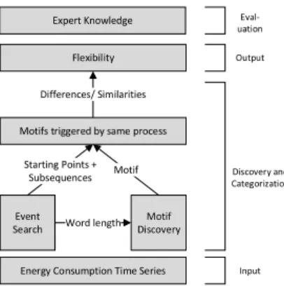
Figure 3: The framework used in this paper to extract flexibility potential from energy consumption data via motif discovery.
always at a different day of the week would indicate that we have a certain flexibility, as to when the process has to start. This is obviously a simplification as we neglect dependencies from other processes at the moment.
2.5 Framework
We use three steps to get to a categorisation of flexibility from steam consumption data before an expert lastly evaluates the potential found. The whole framework is graphically shown in Figure 3. We start with the event search algorithm, saving the subsequences between each event as possible motifs. Afterwards, we run the motif discovery algorithm using the average length of the event subsequences as the word and window length. We then measure the similarity of the found motifs with the subsequences, using dynamic time warping. The motifs which are similar enough are used to examine their differences more closely and categorize their flexibility potential. In the last step, an expert for the processes is needed to evaluate which of the potential flexibilities found can actually be used for flexibility measures and which are due to other factors.
Time Steps
Load in MW
Figure 4: Original time series data of a buildings steam demand over five weeks.
3 Results
To evaluate the proposed method we have a look at the load consumption time series from a building of a chemical factory. The steam consumption is measured as hourly average in tons over a period of five weeks. Due to commercial sensitivity issues, no true measurement values or time indicators will be presented in this paper. Although we do not have information on the products manufactured, we know that there are possibly one or several repeating processes in the factory building. Given this consumption data, we want to find the shapes of those recurring processes. The time series is depicted in Figure 4. Visual analysis of the graph indicates a pattern which repeats itself on different levels of steam intake.
This section presents the individual steps described in the framework, starting with the motif discovery and event search, before analysing and categorizing the flexibility.
3.1 Motif Discovery
Following the framework we have established, we run the above described minima search algorithm with a window size of 100 and store the local minima found in a vector. We then build subsequences of the time series, starting at each of those minima. One subsequence is only five time
Time steps Load in MW Motif d e f
Figure 5: Exemplary subsequences of the steam consumption time series. Each subsequence starts after a minimum detected through the minima event search with a window of size 100.
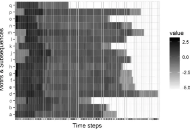
steps long, as all other subsequences are substantially longer, we treated this short one as belonging to the next subsequence. Additionally the sequence until the first minimum is also treated as a subsequence. The minima search gives a very good result to find the different time series subsequences which look similar enough to be from the same batch process. Figure 5 shows some exemplary subsequences found through the event search. The structure of the process seems to remain the same over the different instances. However, the length and intensity of the process vary, which is useful for our purpose as it could be an indicator for flexibility. Figure 6 shows a heatmap of all the subsequences, where
we have normalized all subsequences with mean μ = 0 and standard
deviationσ= 1. The subsequences are aligned at their minimum point.
We can clearly see that they exhibit a similar structure but differ in length.
Next, we run the motif discovery algorithm using the additional informa-tion we have about the processes. We chose a relatively small alphabet
size of a = 10 as the variations in patterns do not seem to be high.
Choosing the word length is more difficult as it has a great impact on
the found motifs. Additional information on thenormal length of the
process running would be the obvious choice for those parameters, which we do not have in our case. However, given the subsequences found in the
Figure 6: Heatmap of the individual subsequences found through the minima search. The subsequences start at the minimum and end at the next minimum. For a better comparison of their structure they are normalized (𝜇= 0, 𝜎= 1). event search, we can now use the mean time distance between the local minima found (w = 94). For the moment we do not allow for overlaps between the motifs.
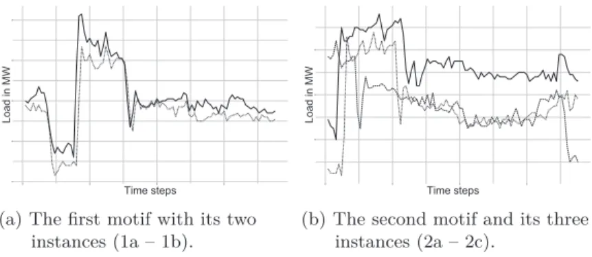
The algorithm finds two different motifs, whose starting points in the time series can be seen in Figure 7. The individual instances of the motifs are displayed in Figure 8. Motif 1 occurs two times in the time series, while Motif 2 occurs three times. There are variations in the motifs, which is helpful for our flexibility examination later. However, they also do not look very different, which lets us assume they might be similar enough to be the same motif if their comparison would start at the minimum as with the event search sequences. All other patterns are classified by the algorithm as not being repeated.
To further investigate this idea, we compare the DTW distances of the motifs within themselves and in between each other. To be comparable, the motifs have all been normalized with mean 𝜇 = 0 and standard deviation𝜎= 1. The result can be found in Table 1. The distances vary between 20.96 and 76.97, with the first one being the distance between the two instances in the first motif and the second one being the distance between the third instance of the second motif and the first instance of the first motif. The third instance of the second motif seems to be the odd one out.
Time Steps
Load in MW
Figure 7: The steam consumption time series with the starting and ending point of the discovered motifs marked by the vertical dotted lines.
Time steps
Load in MW
(a) The first motif with its two instances (1a – 1b).
Time steps
Load in MW
(b) The second motif and its three instances (2a – 2c).
Figure 8: The two motifs found by the motif discovery algorithm.
This result might be to the rather large drop of load at the beginning of the instance. The heatmap depicted in Figure 9 confirms this idea, with the motif in the top row (2c), having a shorter period at a high-level energy intake before dropping. However, we will assume that the distance also for the third instance is small enough for our purposes and so assume that all five instances are triggered by the same mechanism.
As a next step, we want to have a look at the subsequences from the event search. We have seen from the heatmap before, that they all exhibit a similar pattern but differ mainly in length (see Figure 6). We now compare the motifs found through the motif discovery algorithm with the subsequences determined through the event search. It is our aim to find how similar those motifs are to each other. Table 2 shows the difference
Table 1: The dynamic time warping distances for the motifs within themselves. The minimum distance for each motif is highlighted.
Motif 1a 1b 2a 2b 2c 1a 0 20.96 52.51 47.13 76.97 1b 20.96 0 49.04 42.25 75.07 2a 52.50 49.04 0 27.83 59.43 2b 47.13 42.26 27.83 0 59.63 2c 76.97 75.07 59.43 59.63 0
Figure 9: Heatmap of the two motifs found with their respective instances. The motifs are normalized with𝜇= 0 and𝜎= 1.
calculated between each motif found with the motif discovery algorithm (1a – 2c) and the event search subsequences (a – q). As we can see in the table, the distances are for many sequences greater than those for the motifs within themselves. However, we also have some subsequences, where the distances are lower than within the motifs, e. g. subsequence q and motif 2c have a DTW distance of 23.90.
3.2 Flexibility Measures
Given the subsequences which we have found are similar enough to stem from the same underlying process, we now want to determine their flexibility. However, before going further into the analysis of the flexibility we can find by comparing the subsequences according to our
Table 2: The dynamic time warping distances for each subsequence (a – q) with the motifs (1a – 2c), the minimum distance is highlighted.
Motif a b c d e f 1a 89.43 57.26 57.52 62.80 64.21 73.88 1b 93.45 62.16 61.59 65.89 63.81 78.00 2a 63.71 46.32 49.84 48.99 44.44 63.37 2b 70.06 60.01 58.86 62.49 62.87 74.96 2c 44.90 53.19 61.79 50.12 40.87 41.94 Motif g h i j k l 1a 84.65 76.25 50.15 48.50 52.50 46.95 1b 94.78 78.00 53.47 52.31 53.78 46.72 2a 58.19 37.16 50.00 52.37 33.36 46.43 2b 74.75 45.24 42.31 44.16 37.70 32.58 2c 37.07 39.55 71.95 79.56 53.62 70.60 Motif m n o p q 1a 57.39 56.30 44.55 49.01 42.53 1b 58.73 59.77 57.35 50.18 49.43 2a 49.22 39.94 42.81 45.48 23.90 2b 42.19 33.34 52.59 44.18 32.43 2c 62.55 28.45 38.24 62.91 54.49
flexibility measures, we first match the subsequences with the five motif instances. Thus, we will not take the motifs into our analysis if one of the subsequences already describes them.
Table 4: The subsequences and their starting indices, compared to the motifs and their starting indices. All motifs can be reasonably described by a subsequence.
Sub. Start Motif Start Sub. Start Motif Start
a 0 j 913 b 93 k 1015 c 180 l 1103 d 250 m 1205 2b 1223 e 381 2a 377 n 1323 2c 1317 f 491 o 1430 1a 1411 g 599 p 1517 1b 1505 h 706 q 1632 i 805 3.2.1 Energy Flexibility
According to our three measures described before, we inspect the diffe-rences in energy usage from our subsequences. The results are displayed in Table 5. The length of the processes varies between 49 and 131 time steps. However, the intensity for some motifs is rather similar although the lengths differ. This might indicate that no matter how long or short the process is, we need to use roughly the same amount of energy. The ramping time changes considerably between the instances. While the shortest ramping takes only two time steps, the longest takes more than 90 time steps.
Correlation between the length of the process and the intensity as mea-sured by the area under the curve is𝜌= 0.8446, indicating that a longer process also uses more energy. However, ramping steps and the length of Table 4 shows that all motif starting points are reasonably close to starting points of the subsequences. The motifs are included in the subsequences labelled e, m, n, o and p. Hence, we only use these subsequences from now on and use the term motifs for them interchangeably. We analyse the motifs with the help of the above-established flexibility measures. First, we examine the energy flexibility, before delving into the time flexibility.
the process are only slightly positively correlated with𝜌= 0.2832, as are the ramping steps and the intensity𝜌= 0.3649.
Table 5: Characteristics of the found patterns in the steam demand time series. Characteristic Min Median Max StdDev
Length 49.00 102.00 131.00 19.13 Intensity 293.94 294.37 310.97 7.31 Ramping Time 2.00 12.50 90.00 21.68 ● ● ● ● ● ● ● ● ● ● ● ● ● ● ● ● 00:00 01:00 03:00 09:00 11:00 13:00 15:00 17:00 18:00 19:00 22:00 23:00
Fri Mon Sat Sun Thu Tue Wed Figure 10: Starting date and time for each event.
3.2.2 Time Flexibility
Finally, we consider the time flexibility of our sequences. Figure 10 shows the hour and the day of the week where each local minimum is located. As we can see, the weekdays and times of these possible starting points are well distributed throughout the week and day. This indicates that there is no dependency on the weekday or hour of the day to start the process. This might thus be a highly automated process or one with several shifts throughout the day. The fact that there is no clear pattern in the time of the week could mean that we are free to choose the starting point time-wise and thus have a great flexibility there. It could however also imply that the process highly depends on some other variables which we do not consider.
3.3 Categorisation of Flexibility
Given the results in the previous sections, we classify the potential flexibility we get. As we only find potential flexibility at the moment, we cannot infer the technical or economical usability of those flexibilities before consulting an expert. However, we can rank the potential flexibility, and use three different flexibility categories in the following.
The highest available flexibility seems to be in the ramping process. The ramping time is almost independent from the length of the process and only slightly correlated with the intensity of the process. This could indicate that the ramping is flexible as long as we end up at the right intensity at the preferred time point.
The length of the process also varies greatly but is correlated to the intensity. This implies that we can choose whether we start a short or long batch, depending on the energy available.
Lastly, the starting times vary across a wide range, this might indicate that we do not have restrictions considering the time of day when to start a process. As we also have starting times in the middle of the night, we can assume that there are either workers available during the night or this is an automated process. Either way, the starting time can be chosen rather freely. However, as the energy intake of the process is seldom zero, the process either needs a specific amount of energy in a stand-by modus, or the starting time highly depends on what happened before. There might be restrictions as to how long the break between two batches can be, etc.
4 Conclusion and Outlook
This paper proposed a new method to find motifs in industrial batch processes and applied the method to time series of steam consumption data in chemical processes.
The flexibility we find in this paper is only potential flexibility. As we do
not know anything about the process in terms of its technical properties or dependencies of other processes before or after it is running, we only indicate that there might be a potential as there has been some variety in the past. If this variety is only driven by technical features it would not be considered flexibility. Thus, in a next step to properly quantify
the flexibility one has to talk to the process manager and let him rate the potentials found according to their usability. We might also not want to use the flexibility found, even if technically possible, as it is not economically feasible (see Figure 2 for the differences).
Future work will address several aspects of the paper. An investigation of other event search algorithms might be useful, especially if we expect pauses in the processes which are then also a minimum but not an indicator for a process start. Concerning the similarity of the time series sequences, we want to use sequence alignment and flying bricks in a next step. The purpose then being to match the SAX representations of the subsequences and find how the motifs differ and are similar to each other instead of measuring the dynamic time warping distance. This would allow for a more detailed investigation into what can be used for flexibility purposes in the future. Furthermore, we will analyse the potential flexibility and find the real technical and economical flexibility with the help of a process expert. Lastly, given this flexibility, we want to find market mechanisms to encourage the use of flexibility by the process manager whenever this would be more efficient or cheaper. We also want to apply this method to other data and implement it in the Energy Lab 2.0 [11] at a later stage.
Acknowledgements
This work was partly funded by the German Research Foundation (DFG) Research Training Group 2153 “Energy Status Data – Informatics Met-hods for its Collection, Analysis and Exploitation”.
References
[1] L. Barth, N. Ludwig, E. Mengelkamp, and P. Staudt. A comprehen-sive modelling framework for demand side flexibility in smart grids.
Computer Science - Research and Development, 30(4):1758, 2017.
[2] E. Berlin and K. van Laerhoven. Detecting leisure activities with dense motif discovery. In Anind K. Dey, editor,Proceedings of the 2012 ACM Conference on Ubiquitous Computing, pages 250–259,
[3] C. Cassisi, M. Aliotta, A. Cannata, P. Montalto, D. Patanè, A. Pulvirenti, and L. Spampinato. Motif discovery on seismic amplitude time series: The case study of Mt Etna 2011 eruptive activity. Pure and Applied Geophysics, 170(4):529–545, 2013.
[4] G. Chicco. Overview and performance assessment of the clustering methods for electrical load pattern grouping. Energy, 42(1):68–80,
2012.
[5] B. Chiu, E. Keogh, and S. Lonardi. Probabilistic discovery of time series motifs. In Ted Senator, editor,Proceedings of the ninth ACM SIGKDD international conference on Knowledge discovery and data mining, pages 493–498, New York, NY, 2003. ACM.
[6] L. Farinaccio and R. Zmeureanu. Using a pattern recognition appro-ach to disaggregate the total electricity consumption in a house into the major end-uses. Energy and Buildings, 30(3):245–259, 1999.
[7] A. Faruqui and S. Sergici. Household response to dynamic pricing of electricity: A survey of 15 experiments. Journal of Regulatory Economics, 38(2):193–225, 2010.
[8] J. Froehlich, E. Larson, S. Gupta, G. Cohn, M. Reynolds, and S. Patel. Disaggregated end-use energy sensing for the smart grid.
IEEE Pervasive Computing, 10(1):28–39, 2011.
[9] E. F. Gomes, A. M. Jorge, and P. J. Azevedo. Classifying heart sounds using multiresolution time series motifs. In Bipin C. Desai, editor,Proceedings of the International C* Conference on Computer Science and Software Engineering, pages 23–30, New York, NY, 2013.
ACM.
[10] M. Gupta, J. Gao, C. Aggarwal, and J. Han. Outlier detection for temporal data: A survey. IEEE Transactions on Knowledge and Data Engineering, 26(9):2250–2267, 2014.
[11] V. Hagenmeyer, H.K. Çakmak, C. Düpmeier, T. Faulwasser, J. Isele, H. B. Keller, P. Kohlhepp, U. Kühnapfel, U. Stucky, S. Waczowicz, and R. Mikut. Information and communication technology in Energy Lab 2.0: Smart energies system simulation and control center with an Open-Street-Map-based power flow simulation example. Energy Technology, 4(1):145–162, 2016.
[12] C. Lin and C. L. Moodie. Hierarchical production planning for a modern steel manufacturing system. International Journal of Production Research, 27(4):613–628, 2007.
[13] A. Mueen, E. Keogh, Q. Zhu, S. Cash, and B. Westover. Exact discovery of time series motifs. In Haesun Park, editor, Proceedings of the Ninth SIAM International Conference on Data Mining, pages
473–484. SIAM, Philadelphia, 2009.
[14] M. Müller. Information Retrieval for Music and Motion. Springer
Berlin Heidelberg, Berlin, Heidelberg, 2007.
[15] B. Neupane, T. B. Pedersen, and B. Thiesson. Towards flexibility detection in device-level energy consumption. In Wei Lee Woon, editor,Data analytics for renewable energy integration, volume 8817
ofLecture Notes in Computer Science, pages 1–16. Springer, Cham,
2014.
[16] P. Palensky and D. Dietrich. Demand side management: Demand response, intelligent energy systems, and smart loads. IEEE Tran-sactions on Industrial Informatics, 7(3):381–388, 2011.
[17] J. Serra, M. Müller, P. Grosche, and J. L. Arcos. Unsupervised detection of music boundaries by time series structure features. In
Twenty-Sixth AAAI Conference on Artificial Intelligence, 2012.
[18] Y. Simmhan and M. U. Noor. Scalable prediction of energy con-sumption using incremental time series clustering. In Xiaohua Hu, editor, IEEE International Conference on Big Data, 2013, pages
29–36, Piscataway, NJ, 2013. IEEE.
[19] S. Waczowicz, M. Reischl, V. Hagenmeyer, R. Mikut, S. Klaiber, P. Bretschneider, I. Konotop, and D. Westermann. Demand response clustering - how do dynamic prices affect household electricity con-sumption? In2015 IEEE Eindhoven PowerTech, pages 1–6. IEEE,
2015.
[20] S. Waczowicz, M. Reischl, S. Klaiber, P. Bretschneider, I. Konotop, D. Westermann, V. Hagenmeyer, and R. Mikut. Virtual storages as theoretically motivated demand response models for enhanced smart grid operations. Energy Technology, 4(1):163–176, 2016.
Zuverlässigkeitsbasierte Fusion von
Fahrstreifeninformationen für
Fahrerassistenzfunktionen
Tran Tuan Nguyen
1, Jens Spehr
1, Jan-Ole Perschewski
1, Fabian
Engel
1, Sebastian Zug
2, Rudolf Kruse
21Volkswagen AG, 38436 Wolfsburg
E-Mail: {tran.tuan.nguyen, jens.spehr, jan-ole.perschewski, fabian.engel}@volkswagen.de
2Otto-von-Guericke Universität Magdeburg, 39106 Magdeburg
E-Mail: {sebastian.zug, rudolf.kruse}@ovgu.de
Kurzfassung
Eine zentrale Aufgabe für Fahrerassistenzsysteme und autonomes Fah-ren ist die robuste Fahrstreifenerkennung. Dafür müssen Informationen aus verschiedenen Sensoren kombiniert werden, etwa Kameras, Lidars, Radars etc. Die große Herausforderung bei der Fusion verschiedener Informationsquellen besteht darin, dass diese Quellen unterschiedliche Zuverlässigkeiten in unterschiedlichen Situationen aufweisen. Daher stellt diese Arbeit ein Fusionskonzept vor, welches die Zuverlässigkeiten der Quellen berücksichtigt. Dazu wird eine Metrik präsentiert, mit der sich die Qualität einzelner Fahrstreifenerkennungen quantifizieren lässt. An-schließend werden unterschiedliche Klassifikationsverfahren eingesetzt, um Zuverlässigkeiten der Sensoren in verschiedenen Szenarien zu lernen. Anhand der prädizierten Zuverlässigkeiten erfolgt eine adaptive Fusion der verlässlichen Quellen. Anhand experimenteller Erprobungen kann der Nutzen des vorgestellten Konzepts durch eine Performanzsteigerung von bis zu 7% gezeigt werden.
1 Einleitung
In den letzten Jahren rückt automatisches Fahren in den Fokus zahlreicher Forschungseinrichtungen und Unternehmen. Dabei ist die Fahrbahner-kennung eine der entscheidensten Aufgaben. Dazu präsentieren viele