Research Article Efficient Use of Variation in Evolutionary Optimization

(1)

Volume 2010, Article ID 696345,7pages doi:10.1155/2010/696345

Research Article

Efficient Use of Variation in Evolutionary Optimization

John W. Pepper

Santa Fe Institute, 1399 Hyde Park Rd, Santa Fe, NM 87501, USA

Correspondence should be addressed to John W. Pepper,[email protected]

Received 19 July 2009; Accepted 6 January 2010 Academic Editor: Chuan-Kang Ting

Copyright © 2010 John W. Pepper. This is an open access article distributed under the Creative Commons Attribution License, which permits unrestricted use, distribution, and reproduction in any medium, provided the original work is properly cited.

Evolutionary algorithms face a fundamental trade-oﬀbetween exploration and exploitation. Rapid performance improvement

tends to be accompanied by a rapid loss of diversity from the population of potential solutions, causing premature convergence on local rather than global optima. However, the rate at which diversity is lost from a population is not simply a function of the

strength of selection but also its eﬃciency, or rate of performance improvement relative to loss of variation. Selection eﬃciency

can be quantified as the linear correlation between objective performance and reproduction. Commonly used selection algorithms

contain several sources of ineﬃciency, some of which are easily avoided and others of which are not. Selection algorithms based

on continuously varying generation time instead of discretely varying number of oﬀspring can approach the theoretical limit on

the eﬃcient use of population diversity.

1. Introduction

“Premature convergence”, or the loss of diversity before a satisfactory solution is found, is a persistent problem in

evolutionary optimization [1]. This reflects the fundamental

trade-oﬀbetween exploration and exploitation, or between

thoroughness and speed in evolutionary search [2]. If

selection is too weak, progress is slow and many generations are required to find a solution. On the other hand, if selection is too strong, the population rapidly loses diversity and may become stranded on a local fitness peak. A wide variety of techniques have been proposed to address this problem, but it has generally been approached on an ad hoc empirical basis, and little theory has been available to guide the design of selection algorithms.

While the trade-oﬀbetween improving performance and

preserving diversity cannot be avoided, it can be ameliorated

through the eﬃcient use of variation. Diversity within a

population acts as the fuel of the selection process: it is required for selection to act, but is itself consumed in the

pro-cess. However, selection algorithms diﬀer not only in speed,

but also in “fuel eﬃciency”, or rate of improvement relative

to loss of variation. In the following sections, I develop a

method for quantifying the eﬃciency of fitness functions,

defined here as mappings from objective performance to reproduction. (Such mappings are sometimes referred to

as “selection methods”.) The approach is based on the powerful formalism from evolutionary biology known as the “Price equation”, which is increasingly used in evolutionary

genetics [3]. I next compare several widely-used selection

methods to characterize their sources of ineﬃciency, and to

illustrate the advantages of more eﬃcient selection. I also

consider whether less eﬃcient algorithms have any oﬀsetting

advantages that justify their use. Finally, I discuss the design

of fast and eﬃcient fitness functions, and propose a new kind

of algorithm, based on varying generation time instead of

number of oﬀspring, which can approach perfect eﬃciency

in the use of genetic variation.

2. Quantifying Selection Efficiency

The ultimate goal of evolutionary optimization is to maxi-mize some objective measure of performance on a given task. Here I measure progress toward optimization in terms of the mean performance level of the population (In evolutionary computation applications, the ultimate interest may be in the highest performance level in a population of candidate solutions, rather than the mean. However, mathematical theory is only available to quantify change in population mean through selection rather than change in popula-tion maximum. As a practical matter, maximizing mean

(2)

performance will also maximize best performance, all else being equal). The goal of improving performance conflicts partially with a subsidiary goal: maintaining the diverse population of candidate solutions or “individuals” needed to thoroughly explore search spaces and find the best possible solutions. The conflict arises because the unequal repro-duction that drives improvement in average performance also reduce population diversity. Unequal contributions to

the next generation’s gene pool by diﬀerent individuals

always reduces diversity except in the special case of negative frequency-dependent selection (which increases diversity). If selection is frequency-independent, unequal reproduction reduces diversity, in direct proportion to the reproductive variance among individuals (see the appendix).

Although selection cannot improve a population’s aver-age performance in the next generation without unequal reproduction, the converse is not true. Unequal reproduction and resulting loss of diversity need not improve average performance. Variance in reproduction that is uncorrelated with performance can reduce genetic diversity (though

genetic drift) just as quickly as can eﬀective selection, but

without increasing mean performance. Because correlation between performance and reproduction is what makes

selection eﬀective at optimization, I focus on the strength of

this correlation to quantify the eﬃciency of fitness functions.

In addition to selection, genetic operators such as mutation and recombination can also change a population’s mean performance (although in an unpredictable direction).

Here I focus exclusively on the eﬀects of selection, or

diﬀerential reproduction, because this is the source of

premature convergence in evolutionary optimization. Let each individual in the population (indexed by i) have a

measured performance level pi. The average population

performance before selection is p = pi/N, where N =

population size. After one generation of selection, average population performance will be the average of the parent performances weighted by the contribution of each parent

to the next generation: p = piwi/wi, where wi =

the number of oﬀspring produced by the i’th individual.

(Note that this assumes perfect heritability of performance

from parent to oﬀspring.) To simplify the notation, it is

convenient to replace absolute reproductionwiwith relative

reproduction,wi =wi/w, so that mean performance in the

oﬀspring generation isp=ave(piwi). The change in average

performance caused by one round of selection is thenΔp=

p−p, or

Δp=avepw−avep. (1)

As a result of selection, performance improvement across one

generation is exactlyΔpabove. We can rewrite (1) in a useful

form by using two identities: firstly, ave(pw) = ave(p)·

ave(w) + cov(pw), where “cov” represents covariance.

Sec-ondly, ave(w) =1 by definition. With these substitutions,

the improvement in performance from parent to oﬀspring

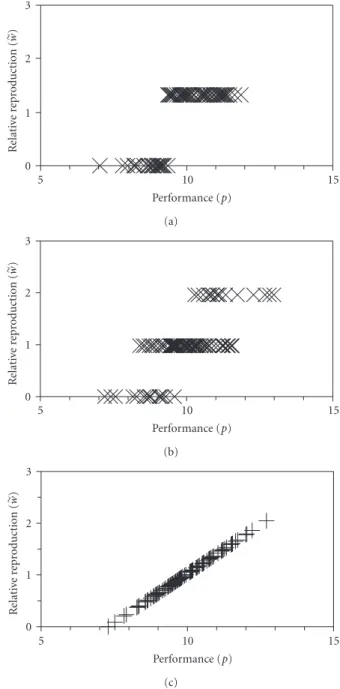
generation is Δp=covp,w (2) 0 1 2 3 R elati ve re pr oduction ( w ) 5 10 15 Performance (p) (a) 0 1 2 3 R elati ve re pr oduction ( w ) 5 10 15 Performance (p) (b) 0 1 2 3 R elati ve re pr oduction ( w ) 5 10 15 Performance (p) (c)

Figure 1: Three fitness functions illustrated using the same set of 100 simulated individuals with performance values drawn from a

normal distribution with mean=10 and standard deviation=1.

(a) threshold selection (b) stochastic proportionate selection (SPS),

(c) deterministic proportionate selection (using (8)). Each mark

represents one individual.

(see [4]). To highlight the factors aﬀecting optimization rate,

it is useful to use another identity to rewrite this covariance as a product of its three factors:

Δp=σp·σw·ρpw, (3)

where σis a standard deviation among individuals in

performance (p) or relative reproduction (w), andρpwis the

linear correlation coeﬃcient between the two [4].

Equation (3) provides insight into how to maximize

(3)

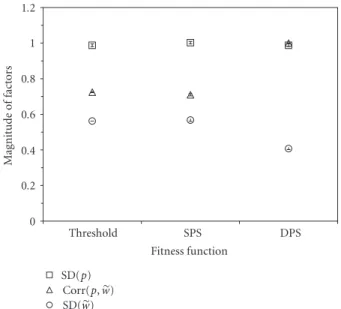
0 0.2 0.4 0.6 0.8 1 1.2 M ag nitude o f fact o rs Threshold SPS DPS Fitness function SD(p) Corr(p,w) SD(w)

Figure 2: The three factors contributing to performance improve-ment compared over 1 round of selection across three fitness func-tions using numerical simulafunc-tions: threshold selection, stochastic proportionate selection (SPS), and deterministic proportionate selection (DPS). Each sample consisted of 100 simulated individuals with performance values drawn from a normal distribution with

mean = 100, SD = 1. Markers show means, and bars show ±

standard error over 100 samples. (Note that error bars are too small to extend beyond marker symbols.)

−8 −6 −4 −2 0 2 4 Change (%) Threshold SPS DPS Fitness function Performance (p) Diversity (H)

Figure 3: The same three fitness functions shown in Figure 2

compared for the one-generation change produced in mean performance, and in population diversity. Bars show standard errors. (Note that error bars are too small to extend beyond marker symbols).

to loss of diversity. Deviation in individual performance (σp)

is fixed for a given population, butσw andρpw depend on

the selection method. Deviation in reproduction (σw) varies

with the strength of selection. Increasingσw can increase

performance improvement, but at the cost of faster loss of diversity. The linear correlation between performance and

reproduction (ρpw) corresponds to the eﬃciency of selection,

in the sense that increasing this term increases performance improvement without increasing loss of diversity and

per-formance variation. Whenρpw =0, selection is completely

ineﬃcient: it consumes variation without improving average

performance. In the language of evolutionary theory, this is termed “drift” instead of “selection”. At the other extreme

ofρpw= 1, the ratio of performance increase to variance

reduction is maximized. Thus the rate at which variation is lost from a population is not simply a function of selection

strength (σw), as is sometimes assumed, but also of selection

eﬃciency (ρpw).

3. Sources of Inefficiency in Fitness Functions

The perfectly linear fitness function (ρpw=1) is an ideal of

eﬃciency that is not realized by any algorithm in general

use. All standard fitness functions depart from linear correla-tion either through deterministic nonlinearities, fluctuating stochastic nonlinearities, or both. An example of a deter-ministically nonlinear fitness function is threshold selection, in which reproduction is an all-or-nothing step function

of performance (Figure 1(a)). Any such highly nonlinear

fitness function will necessarily have a linear correlation well below 1. Fitness functions without any deterministic nonlinearity are termed “fitness-proportionate selection” because expected reproduction is directly proportional to

performance [1]. However, these functions introduce

fluctu-ating stochastic nonlinearity in converting expected to actual reproduction, so that expected reproduction has perfect linear correlation with performance, but actual reproduction does not. This is hard to avoid because unlike the expected

number of oﬀspring, the actual number of oﬀspring is

con-strained to whole numbers and so must vary stochastically around the expected number. For example, the commonly

used “stochastic universal sampling” algorithm [5] works as

follows: an expected reproduction of ωis partitioned into

a fractional portion (ω%1) and a whole-number portion

[ω−(ω%1)], where % is the modulo operator. The algorithm

produces the whole number of oﬀspring, plus one additional

oﬀspring with a fractional probability of (ω%1). Despite its

lack of deterministic nonlinearity, the correlation between

performance and actual number of oﬀspring is less than 1

because of stochastic fluctuations (e.g., Figure 1(b), where

ω=1 for each individual, butwvaries stochastically). I will

refer to this algorithm as “stochastic proportionate selection” (SPS).

Such stochastic fluctuations in actual reproduction are larger in other implementations of fitness-proportionate

selection, such as “roulette wheel” sampling [2]. Still other

algorithms, such as tournament selection [1], include both

(4)

selection of a pair of individuals to compare is stochastic, while the choice of which of the two reproduces depends on their relative performance rank, which is a deterministic nonlinear function of performance. Both deterministic and stochastic nonlinearities in fitness functions reduce the correlation between performance and actual reproduction,

and thereby reduce selection eﬃciency.

To examine the eﬀect of selection eﬃciency on diversity,

I used a numerical simulation consisting of a population of 100 individuals (candidate solutions) with performance

values drawn from a normal distribution with mean =

10 and standard deviation = 1. I compared the eﬀects

of a single round of selection using threshold

selec-tion (Figure 1(a)), stochastic proportionate selection (SPS)

(Figure 1(b)), and deterministic proportionate selection

(DPS) ((8),Figure 1(c)). The numerical simulation allowed

fractional oﬀspring, but the problem of how deterministic

proportionate selection can be implemented with whole

numbers of individuals is deferred to Section 6 below.

To tune the threshold fitness function to give the same performance improvement as the other two functions, I allowed reproduction only by the best-performing 76% of the population. Deterministic proportionate selection generated less variance in reproduction than the other two, but reproduction was more highly correlated with

performance (Figure 2). These two diﬀerences resulted in an

equal performance increase in the oﬀspring generation for

all three fitness functions (Figure 3). Thus the deterministic

proportionate selection function consumed less performance variation while producing the same performance improve-ment. I next investigated whether DPS also preserved more genotype diversity while producing the same performance improvement.

To quantify diversity, I used the Shannon-Weiner diver-sity index from evolutionary biology, which is equivalent to the entropy of the genotypes in the population:

H= −

g

fglog₂fg, (4)

wheregindexes the genotypes in the population, and fgis the

population frequency of genotype g. Entropy is maximized when each individual is unique, and minimized when all individuals share the same genotype. To simplify calculations I assumed that each individual in the population was unique prior to selection, but violating this assumption would not change the outcome qualitatively. Selection reduced diver-sity several-fold less under the deterministic proportionate function than under either the stochastic proportionate or threshold functions, while improving performance at the

same rate (Figure 3).

4. Is Inefficient Selection Ever Useful?

I have focused here on the advantages of linear fitness functions for conserving genetic diversity. However, both

deterministic nonlinearities and stochastic eﬀects have some

potential advantages. Might these justify the use of nonlinear

fitness functions despite their lower eﬃciency?

Deterministically nonlinear fitness functions permit

stronger selection (higher σw) than linear functions. At

the extreme, reproduction by only the individual(s) with the highest performance increases average performance by

Δp = pmax − p. More generally, larger one-generation

improvements are possible with nonlinear than with linear fitness functions. However, this rapid short-term improve-ment comes at the cost of the variation required for longer-term improvement. Genetic variation could be created anew in each generation, but this is computationally expensive and

reduces evolutionary search algorithms to ineﬃcient

hill-climbers. For this reason, deterministic nonlinearity in fit-ness functions is unlikely to be helpful in most applications.

Stochastic fitness functions oﬀer a diﬀerent potential

advantage by helping populations escape from local per-formance peaks. Slightly deleterious mutations can persist or spread under stochastic selection, making it possible for populations to cross low-performance fitness valleys

requiring multiple mutations. Stochastic eﬀects also allow

the population to drift among diﬀerent genotypes with equal

performance. This may facilitate the exploration of “neutral networks” in genotype space, leading to the discovery of

higher performance peaks [6]. However, stochastic eﬀects

on reproduction also have drawbacks. They can push populations away from global as well as local peaks. In some algorithms, they may also slow the discovery of higher-performance peaks by allowing beneficial new mutations to be lost. It remains an open question how often stochastic fitness functions improve evolutionary optimization, and how much stochasticity is desirable. To investigate these questions, it will help to have algorithms in which stochastic

eﬀects can be directly controlled by the experimenter rather

than being a by-product of the particular algorithm used. This is easily achieved by adding a stochastic term to a deterministic linear fitness function. This approach has the

additional advantage that stochastic eﬀects can be reduced to

any desired magnitude without incurring a computational cost. In contrast, intrinsically stochastic algorithms require

very large population sizes to drive stochastic eﬀects to low

levels.

5. Fast and Efficient Fitness Functions

How can a fitness function be designed to maximize the rate

of performance increase while also optimizing eﬃciency?

Eﬃciency defined as the linear correlationρpwis maximized

when reproduction is a linear function of performance. It is convenient to represent such fitness functions in the standard linear form:

wi=api+b, (5)

where piandwiare individual performance and

reproduc-tion, respectively, and a and b are system parameters. With discrete generations, it is usually desirable to maintain a stable population size across generations, which constrains

(5)

the average number of oﬀspring per individual (w) to 1. This

constrains the value ofato

a= 1

avepi+b =

1

p+b. (6)

Substituting (6) into (5) gives us a linear fitness function

yielding a stable population size:

wi=

pi+b

p+b. (7)

What value of b will maximize the rate of performance

improvement? Recall from (3) that the one-generation

improvement in average performance due to selection is a

product of three quantities:σp,ρpw, andσw. The first of these

is a fixed property of the population. The second is already maximized at 1 under linear fitness functions. This leaves

only variance in individual reproductionσwto be maximized

in order to maximize the performance improvement Δp.

When wi is a linear function of pi, its variance σw is

maximized by maximizing the slope of the fitness function,

which is defined in (5) as a. Equation (6) shows that a

increases as b approaches −p, so thatb should be as close

as possible to−pto maximize improvement. However, there

is a constraint that individual reproduction (wi) cannot be

negative, which means that b ≥ −pi for all i (5). If the

worst performance in the population is denoted aspmin, then

the lowest possible value for b is −pmin, which results in

the individual(s) with the lowest performance having exactly

zero oﬀspring. Substituting this value for binto (7) yields

the stable linear fitness function with the maximum rate of performance increase: wi= pi−pmin p−pmin . (8)

6. A Variable-Generation Algorithm for

Efficient Selection

If a deterministic linear fitness function is the theoretical ideal, how can it be implemented in practice? As discussed

above, ineﬃciency in commonly used fitness functions

arises in part from easily avoidable sources of nonlinearity. However, all standard algorithms also contain nonlinearities arising from the fact that performance is a continuous

vari-able, while the number of oﬀspring is discrete. Stochastically

converting real numbers of expected oﬀspring to whole

numbers of actual oﬀspring reduces the linear correlation

between performance and actual reproduction.

We can overcome this problem by recognizing that selec-tion on genotypes acts through their rate of reproducselec-tion

per unit time. Instead of varying the number of oﬀspring,

one can independently vary the generation time for each

individual [7]. This requires an algorithm incorporating

overlapping generations and a continuous representation of time. Individual reproductive rates can then vary continu-ously rather than discretely, and can correlate perfectly with individual performance.

To implement this idea, individual reproduction is treated as a growth rate, by analogy with population growth rates. A population growth rate tells us how large a population will be after a given time:

st=s0wt, (9)

wheres0 is initial population size,st is population size after

ttime units, andwis growth rate. Rearranging (9) tells us

how long it will take the population size to change by a given

factorst/s0under a given growth ratew:

t=ln(st/s0)

ln(w) . (10)

Our current problem concerns individuals rather than populations, but we can use the same reasoning to ask how long it will take an individual to die (equivalent to shrinking to size zero) or reproduce (equivalent to doubling

in size) as a function of its individual growth ratewi. Because

individuals are discrete, we round oﬀ individual “size” to

the nearest whole number. Thus forwi < 1, we can ask

how long it will take for the individual to fall below half its initial size, given its negative growth rate. At this point, the individual’s size is closer to zero than one, and we recognize this by removing it from the population. Similarly, if an individual’s growth rate is greater than one, we ask how long it will take for its size to rise above 1.5. At this point it is closer to being two individuals than one, and we recognize this by doubling it via reproduction. (Note that

unlike rounding the number of oﬀspring under stochastic

fitness-proportionate algorithms, rounding individual size to whole numbers is not stochastic and does not introduce stochastic nonlinearity into the fitness function. Because waiting times vary continuously, genotype growth rates also vary continuously as a deterministic linear function of performance.)

Forw <1, waiting time to death is found by substituting 0.5

forst/s0in (10), giving

td= −0.693

ln(w) . (11)

For w > 1, waiting time to reproduction is found by

substituting 1.5 forst/s0, giving:

tr= 0.405

ln(w). (12)

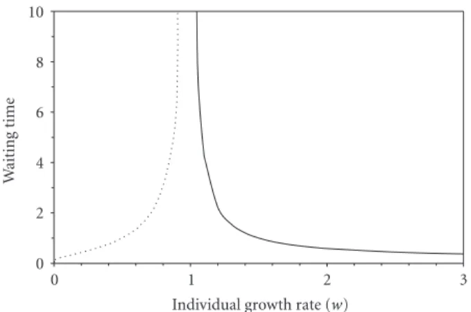
When an individual’s reproductive rate is evaluated, its future death or reproduction is scheduled for a time point in the future designated as a real number on a time line. These events will be scheduled in the distant future when the reproductive rate is close to 1, and in the near future when it

is far from 1 (Figure 4).

At the beginning of a run, each individual’s performance is evaluated and its reproduction or death is scheduled. After this, the algorithm simply consists of repeatedly cycling through the following steps: (1) carry out the first event on the schedule. (2) If the event was a birth, evaluate the new individual’s performance. (3) recalculate all waiting times

(6)

0 2 4 6 8 10 W aiting time 0 1 2 3

Individual growth rate (w)

Figure 4: Waiting time to death (dotted line) or reproduction (solid

line) as a function of individual growth rate. (From (11) and (12).)

to reflect the new average performance, and update the schedule. In practice, it might be useful to recalculate waiting times less often in order to reduce the computational load. For example, each individual’s waiting time could be calcu-lated at birth and then not recalcucalcu-lated until its scheduled event was within some specified time horizon.

7. Conclusions

In these results, truly linear fitness functions, in the form of deterministic proportionate selection, reduced population diversity and performance variation less than other fitness functions that improve performance the same amount in one round of selection. This strongly suggests that over multiple generations, the same rate of performance improvement would be sustained with less loss of diversity. Consequently, DPS should yield better solutions, particularly for tasks where premature convergence is otherwise a problem. The variable-generation algorithm outlined above allows actual reproductive rates to be exactly proportional to performance, providing one way to implement DPS. Although stochastic fitness functions may eventually prove useful on some fitness landscapes, intrinsically linear fitness functions provide the best foundation for designing them because they allow stochastic terms to be added in a controlled fashion.

One important caveat is that these conclusions are based on consideration of a single round of selection in

isolation. Longer-term selection is also aﬀected by the

genetic operators that create variation, such as mutation and recombination, and by their interactions with selection. In particular, this paper does not address the issue of how selection interacts with recombination among epistatic

loci (e.g., [8]). While I am not aware of any reason the

conclusions reached here would not hold in the broader context of long-term evolution with recombination; this remains to be investigated.

Appendix

The purpose of this appendix is to quantify the extent to which unequal reproduction reduces diversity in a

population. It will show that when selection is frequency-independent, unequal reproduction reduces diversity in direct proportion to the reproductive variance among

indi-viduals. I followSection 3above in quantifying diversity with

the Shannon-Wiener diversity index, which is equivalent to the entropy of genotypes.

Before selection, variance in the frequencies of alternative genotypes is

varf=Ef2₋_E_f2

, (A.1)

and after one round of selection it is

varw f =Ew2_f2₋_E_{w f} 2

, (A.2)

where variance (var) and expectation (E) operate across

genotypes, f is the frequency of each genotype, and w is

the reproduction of each genotype relative to the population

mean. If selection is frequency-independent, thenwand f

are independent, so that (A.2) can be rewritten as

varw f =Ew2_·_E_f2₋ _E(_w₎2_·

Ef2. (A.3)

Because E(w)=1 by definition, (A.3) simplified to

varw f =Ew2_·_E_f2₋_E_f2

. (A.4)

LetΔvar(f) represent the change in var(f) caused by one

round of selection. Subtracting (A.1) from (A.4) gives

Δvarf=Ef2_·_E_w2₋₁_. _(A.5)

Because E(w)=1, the second term on the right, E(w2₎₋₁₌

E(w2₎₋_[E(_w_)]2₌_var(_w_{). Substituting var(}_w_{) for E(}_w2₎₋₁

gives

Δvarf=Ef2_·_var(_w₎_. _(A.6)

Thus the decrease in the variance of genotype frequencies is proportional to the variance in reproduction. Thus minimizing variance in reproduction also minimizes loss of

diversity (H).

Acknowledgments

This work was supported by and carried out at the Santa Fe Institute. The author thanks H. Bagheri-Chaichian, L. Pagie, and C. Shalizi for helpful discussions, and John. H. Holland for comments on an earlier draft, as well as for suggesting the idea of variable-generation selection methods.

References

[1] M. Mitchell, An Introduction to Genetic Algorithms, MIT Press, Cambridge, UK, 1996.

[2] J. H. Holland, Adaptation in Natural and Artificial Systems, University of Michigan Press, Ann Arbor, Mich, USA, 1975. [3] S. A. Frank, “George Price’s contributions to evolutionary

genetics,” Journal of Theoretical Biology, vol. 175, no. 3, pp. 373– 388, 1995.

(7)

[4] G. R. Price, “Selection and covariance,” Nature, vol. 227, pp. 520–521, 1970.

[5] J. E. R. Baker, “Reducing bias and ineﬃciency in the selection

algorithm,” in Proceedings of the 2nd International Conference

on Genetic Algorithms and Their Applications, J. J. Grefenstette,

et al., Ed., pp. 14–21, Erlbaum Associates, Hillsdale, NJ, USA, 1987.

[6] W. Fontana and P. Schuster, “Continuity in evolution: on the nature of transitions,” Science, vol. 280, no. 5368, pp. 1451– 1455, 1998.

[7] J. H. Holland, “Building blocks, cohort genetic algorithms, and hyperplane-defined functions,” Evolutionary Computation, vol. 8, no. 4, pp. 373–391, 2000.

[8] J. W. Pepper, “The evolution of evolvability in genetic linkage patterns,” BioSystems, vol. 69, pp. 115–126, 2003.

(8)

Submit your manuscripts at

http://www.hindawi.com

Computer Games Technology

International Journal of

Hindawi Publishing Corporation

http://www.hindawi.com Volume 2014

http://www.hindawi.com Volume 2014 Distributed Sensor Networks International Journal of Advances in

Fuzzy

Systems

Reconfigurable Computing

Applied

Computational

Intelligence and Soft

Computing

Advances in

Artificial

Intelligence

Hindawi Publishing Corporation http://www.hindawi.com Volume 2014 Advances in Software Engineering Hindawi Publishing Corporation

Electrical and Computer Engineering

Journal of

Computer Networks and Communications

Hindawi Publishing Corporation

http://www.hindawi.com Volume 2014

Multimedia

Biomedical Imaging

Artificial

Neural Systems

Advances in

Robotics

Journal of

http://www.hindawi.com Volume 2014 Hindawi Publishing Corporationhttp://www.hindawi.com Volume 2014

Computational Intelligence and Neuroscience

Modelling & Simulation in Engineering Hindawi Publishing Corporation

The Scientific

World Journal

Human-Computer Interaction Advances in Computer EngineeringAdvances in