Bankruptcy prediction with support vector machines

(1)

Bankruptcy Prediction with Support Vector Machines: An

Application for German Companies

Master Thesis Submitted to

Prof. Dr. Wolfgang K. Härdle

Linda Hoffmann

Ladislaus von Bortkiewicz Chair of Statistics C.A.S.E.- Centre for Applied Statistics and Economics

Humboldt-Universität zu Berlin

by

Ceren Önder

(521872)

in partial fulfillment of the requirements for the degree of

(2)

(3)

Acknowledgment

I would like to express my deep and sincere gratitude to my supervisor, Prof. Dr. Wolfgang K. Härdle, for his important support and encouragement throughout this work. Many thanks also to my advisor, Linda Hoffmann, for her constructive criticism and insightful comments in all the time of writing my thesis which definitely enabled me to develop a deep understanding of the subject.

I would like to extend my thanks to my brother, Asim Önder, who has made available his kind support in a number of ways. I am indeed grateful to him for spending his time in helping me to finish this work with the best possible results. My sincere thanks also go to my best friend, Damla Kardes, for being with me all the time from the initial to the final level of this work. Her loving support has been of great value.

Last but not the least, I would like to thank my parents, Gonca and Süleyman Önder, for sup-porting me spiritually throughout my life. Without their understanding and encouragement it would have been impossible for me to accomplish this work.

(4)

Abstract

This work investigates the application of support vector machines (SVMs) for prediction of German companies’ failure that is based on 24 financial ratios being grouped into four categories, namely profitability, leverage, liquidity and activity. SVMs, one of the efficient supervised learning methods, can be applied to classification or regression. In our frame-work, we will use SVMs as a classifier to discriminate solvent and insolvent companies. To select the appropriate model composed of the most powerful financial ratios in classifica-tion both forward and backward stepwise selecclassifica-tion techniques are utilized and the derived results are compared through their accuracy ratios. Furthermore, with the use of the same financial ratio data we predict companies’ probability of default via logistic regression. The selection of the regression model is based on Akaike’s information criterion. Then, the best established results of the SVM and logistic models are assessed via their Lorenz curves to figure out which model is more successful method to extract useful information from financial ratios for default prediction. The results release that the SVM model outperforms logistic regression.

Keywords:Financial Ratio, Default Probability Prediction, Support Vector Machines, Lo-gistic Regression

JEL classification:G33, C45 ,C14, C44

(5)

Zusammenfassung

Diese Arbeit untersucht die Anwendung von Support Vektor Machines (SVMs) zur Vorher-sage der Insolvenz von deutschen Unternehmen. Die VorherVorher-sage basiert auf 24 finanziellen Kennzahlen, die in vier Kategorien unterteilt sind: Profitabilität, Fremdfinanzierung, Liqui-dität und Aktivität. SVMs ,eine der effizientesten geordneten Lernmethoden, können zur Klassifikation oder zur Regression dienen. In unserem Fall, werden wir SVMs als Klassifi-kator benutzen, um solvente und insolvente Unternehmen zu diskriminieren. Um das geeig-netste Model, das aus den aussagekräftigsten finanziellen Kennzahlen zusammengesetzt ist, auszuwählen, werden sowohl vorwärts, als auch ruckwärts schrittweise Selektionstechni-ken verwendet, und die hergeleiteten Resultate werden durch ihre Genauigkeitsquote. Des Weiteren nutzen wir die gleichen finanziellen Kennzahlen, um die Insolvenzwahrschein-lichkeit der Unternehmen mit einer logistischen Regression vorherzusagen. Die Wahl des Regressionsmodels basiert auf Akaikes Informationskriterium. Die jeweils besten Resul-tate der SVM und des logistischen Models werden anhand der Lorenzkurve verglichen, um herauszufinden, welches Model erfolgreicher darin ist, wesentliche Informationen für Insolvenzhervorsagen aus den finanziellen Kennzahlen zu ziehen. Die Resultate des SVM-Models übertreffen diejenigen der logistischen Regression.

(6)

(7)

1 Introduction

It is required for any company, private or public, to have funds to run. In the case of insuf-ficient means to meet liabilities, the management of the company will have to liquidate the company’s assets, but when there are not enough funds to repay all debtors fully, the declaration of bankruptcy can happen. Since corporate liabilities have default risk, for the banking indus-try and financial institutions it is essential to discriminate the non-defaulting companies from defaulting ones. Through a good discrimination they can make lending decisions and pursue better pricing strategies and so cover against the counter party risk. To do that these institutions develop their own models relying substantially on statistical tools. Nonetheless, it is not easy to model the relevant risk accurately so that even small miscalculations of the risk can impede the profitability of lending. Having an accurate model to predict corporate failure is of great interest to a variety of parties, such as, insurers, factors, financial analysts and academics. Be-cause of the fact that unexpected realizations of default risk can destabilize and destroy lending institutions, it will always be crucial to improve bankruptcy prediction accuracy.

The problem of prediction of company failure is not a new topic. To the contrary, it has al-ready been analyzed since the 19th century. Similarly, the question of "How can financial data contribute to our understanding of why some firms go into bankruptcy?" has been more than a century old. Ramser and Foster (1931), Fitzpatrick (1932) can be counted as the first scientists applying financial ratios so as to predict company bankruptcy. Nonetheless, Aziz et al. (1988) criticized the models which built bankruptcy prediction on financial ratios. They claimed that corporate bankruptcy is highly related to firm valuation and that is why a cash flow model can predict corporate failure more accurately. Similarly, Sierra and Bechetti (2003) investigated non-financial explanatory variables in order to predict company failure, such as the degree of relative firm inefficiency, customers’ concentration and the strength and proximity of competi-tors.

In the late 1960s, discriminant analysis (DA) was introduced as the first applied statistical tech-nique to bankruptcy prediction. The publications of Beaver (1966) and Altman (1968) are the first works using this method. Afterwards, a variety of models have been developed via us-ing techniques such as logit, probit, hazard models, recursive partitionus-ing and neural networks. Beaver (1966) introduced the univariate DA and provided empirical verification that certain financial ratios, most importantly cash flow to total debt ratio, gave statistically significant sig-nals well before actual business failure occurs. Furthermore, in predicting company failure he stressed that accounting data are crucial and he found that market-value variable and financial ratio are equally reliable. Altman (1968) improved Beaver’s univariate analysis through devel-oping a discriminant function which allows for simultaneous consideration of several ratios in a multivariate analysis, namely multivariate DA, in order to predict company default and he concluded that some of the ratios he used outperformed Beaver’s cash flow to total debt ratio. Altman asserted that an analysis with just one financial ratio at a time is not sufficient in failure prediction. For example, according to him a firm posing a poor picture in terms of profitability

(10)

1 Introduction

may be regarded as having high risk of bankruptcy. Nevertheless, other financial indicators such as above average liquidity can change this adverse situation. Later on, Altman et al. (1977) de-veloped Z-score model for predicting corporate bankruptcy which became a control measure for the financial distress status of the companies. The Z-score is calculated by a linear combination of several common business ratios which are weighted by coefficients. Thanks to its simplicity, it is still widely used in bankruptcy prediction.

Beaver and Altman used financial ratios in order to predict failure of medium and large asset size firms while ignoring small businesses due to the difficulties in acquiring the data. In contrast, Edmister (1972) claimed that bankruptcy is a more common phenomenon for small companies and analyzed the prediction of small business failure by using financial ratios.

Linear probability and multivariate conditional probability models, Logit and Probit, were uti-lized in the corporate failure prediction literature of the late 1970s. The odds of a corporate failure was estimated with the probability via these methods. Martin (1977) introduced "Early warning of bank failure", wherein a logit regression approach is implemented. Later, Moro et al. (1980)’s work of "Financial ratios and the probabilistic prediction of bankruptcy" based on logit model was published, where he used a large sample,105 bankrupt firms and 2,058 non-bankrupt firms, being different from the previous studies. The drawback of this study is that he disregarded the statements after bankruptcy. Some of the other researchers applying logistic and probit model to bankruptcy analysis can be counted as Wiginton (1980), Zavgren (1983) and Zmijewski (1984). As to the other statistical methods used to predict company failures, there are namely gambler’s ruin model (Wilcox (1971)), option pricing model (Merton (1974)), recursive partitioning (Frydman et al. (1985)), neural networks (Tam and Kiang (1992)) and rough sets (Dimitras et al. (1999)).

Wilson et al. (1999) asserted that the contribution of the ability and willingness of a firm to pay its creditors to credit analysis is highly important. In their model, they used a linear combination of financial ratios grouped into categories of liquidity, leverage, business activity and profitabil-ity along with variables obtained from non-financial and payment behavior information, such as company age, company size and industry type. They concluded that the inclusion of a history of payment behavior and non-financial data to the models can improve the bankruptcy prediction. In 2001, Shumway criticized single-period models so-called static models and claimed that through applying these models one can only produce probabilities that are biased and incon-sistent. According to him, firms change through time and static models do not control firms’ risk for each time period. Hence, Shumway and Hope (2001) suggested a hazard model, a multi-period assessment, including time-varying explanatory variables so as to catch the chang-ing company status over time. Furthermore, Glennon and Nigro (2005) suggested a hazard or survival analysis. Similarly, Duffie et al. (2007) predicted corporate distress via multi period model, and they also incorporated the dynamic of firm-specific and macroeonomic covariates. They found the strong dependence of company health status on the current state of the economy and the current leverage of a company.

As to the SVM model introduced by Cortes (1995), it is a supervised learning method based on mathematical programming theory which can be applied to both classification and regres-sion analysis to model and predict corporate failure. Fan and M. (2000), Min and Lee (2005) and Shin et al. (2005) can be given as examples for the previous studies using this method in bankruptcy prediction. In this work, through using Gaussian radial basis function (RBF) as a kernel trick we will use SVMs as a nonlinear classifier to separate solvent and insolvent

(11)

panies. Thanks to kernel trick we will transform the financial ratios into a higher dimensional space where linear separation of the companies is possible.

The remainder of this paper is structured as follows. In Section 2, the important effect of Basel Accords on the financial system is described. The use of the SVM model in bankruptcy prediction is then explained in detail with its related algorithm in Section 3. In Section 4, we present the logistic regression in corporate failure prediction. We render how we clean data and then select the appropriate model for the SVM in Section 5. We provide the empirical results in Section 6 and we conclude in Section 7.

(12)

(13)

2 The effect of Basel Accords on the

financial system

It is also required to glance at the importance of bankruptcy analysis in a broader sense. For a society, it is crucial to have an efficient bankruptcy system. When the efficiency of an applicable bankruptcy system surges, interest rates decline, which leads to increase in creditor payoffs and decrease in cost of debt capital. This fall in cost of debt capital raises the firms’ share of good state returns. With an efficient bankruptcy system the firms have more investment incentives, since the firms decide to carry out projects in an effort to maximize net expected profits which soar when the interest rate decreases. All in all, an efficient bankruptcy system has a major role in stabilizing financial markets which also gives rise to stable inflation and sustainable growth. It is required to have clear and consistent rules which govern the process aiming to have a more stable financial system. In this respect, the role of the Basel Committee on Banking Supervision (BCBS) being established as an international committee by the Bank for International Settlements is of great importance for financial system, because it aims to strengthen supervisory and risk management practices globally.

BCBS disclosed Basel I, the first Basel Capital Accord, in 1988 which was enforced by law in G-10 countries in 1992. Basel I mainly focused on credit risk. The ultimate aim was to determine capital standards and to ensure that banks have a sound amount of capital. It required the banks with international presence to possess a minimum capital to risk weighted asset ratio of 8%. Holding a certain amount of capital is crucial because of the fact that capital of financial institutions is the last guard against bank insolvency.

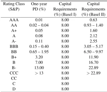
Because of the developments in financial innovations and risk management BSBC started in 2000 working on Basel II to create more comprehensive and risk sensitive set of guidelines to capital adequacy. Within this Accord being revised in 2004 one-size-fits-all methodology for computing capital ratio was transformed to a set of three choices; the standardized approach, the internal ratings-based approach (IRB) and the advanced internal ratings-based approach (AIRB). The difference from one-size-fits-all methodology is that IRBs allow the participating financial institutions to utilize their own internal estimates of risk components in determining the capital requirement to guard against financial and operational risk. Importantly, BSBC added operational risk into the capital to assets ratio. In short, the aim of Basel II is to set an international standard to determine the amount of capital that banks require to hold in order to protect themselves against financial and operational risks. Such an international standard can guard international system from major banks collapse. When a bank puts aside capital reserves in parallel to the risk in its lending and investment activities, this will lead to economic stability. The greater this risk, the greater the amount of capital the bank requires to hold in order to protect its solvency. It is obvious that, this point differs from Basel I which required banks to have minimum capital amount of 8%. The difference between two Basel Accords can be seen in Table 2.2.

(14)

2 The effect of Basel Accords on the financial system

Rating Class (Moody’s) Four year PD (%)

Aaa 0.02 Aa2 0.05 Aa3 0.11 A1 0.21 A2 0.38 A3 0.59 Baa1 0.91 Baa2 1.32 Baa3 2.62 Ba1 4.62 Ba2 7.48 Ba3 10.77 B1 15.24 B2 19.94 B3 26.44 Caa1 35.73 Caa2 72.87 Caa3 48.27 Ca 100.00 C 100.00

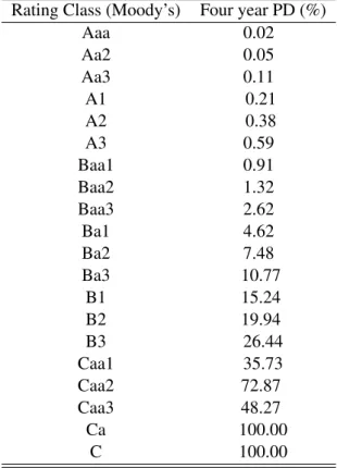
Table 2.1: PDs used in rating structure finance securities. Source: Moody’s Rating Methodol-ogy (2006)

As a new update to the Basel Accords, in September 2010 BCBS announced the Basel III which was confirmed by the G-20 in November 2010 at Seoul G-20 leaders’ summit. New Basel Ac-cords aim to strengthen capital and liquidity requirements in response to the last global financial crisis stemmed from the mortgage and credit crunch in the US. In addition, the required capi-tal conversation buffer will also be increased which is crucial to ensure that banks have capicapi-tal buffer that can cover losses during the periods of financial and economic distress. Introduction of a global liquidity standard and new capital buffers with tightened minimum common equity requirement are important financial sector reforms supporting the economic growth. Obviously, the goal is to make the financial firms stronger against future financial crises.

A company’s bond rating reflects its financial strength which is negatively correlated to the cost of debt. Cost of debt is the yield to maturity on the company bonds or simply the cost of borrowing money. Therefore, the higher the company rating, the higher company’s ability is to make repayments of interest and principal; in other words, the cost of debt will be lower for a high rated company. The most important credit rating agencies are Moody’s, Standard and Poor’s and Fitch IBCA that publish ratings in the US. Moody’s rating methodology disclosed in 2006 for four year PDs is given for an example in Table 2.1.

As the Basel Accords emphasize, it is important for a bank or any other financial institution to quantify the risk of insolvency of the borrower. At this point, which rating method is the most accurate one to discriminate the low-risk and high-risk companies becomes important. If financial institutions can find the adequate model, they can invest in low-risk companies and

(15)

Rating Class One-year Capital Capital

(S&P) PD (%) Requirements Requirements

(%) (Basel I) (%) (Basel II)

AAA 0.01 8.00 0.63 AA 0.02 – 0.04 8.00 0.93 – 1.40 A+ 0.05 8.00 1.60 A 0.08 8.00 2.12 A- 0.11 8.00 2.55 BBB 0.15 – 0.40 8.00 3.05 – 5.17 BB 0.65 – 1.95 8.00 6.50 – 9.97 B+ 3.20 8.00 11.90 B 7.00 8.00 16.70 B- 13.00 8.00 22.89 CCC >13 8.00 >22.89 CC 8.00 C 8.00 D 8.00

Table 2.2: Rating grades and capital requirements. Source: Damodaran (2002) and Fuser (2002). The authors estimated the figures in the last column for a loan to a small and medium enterprise with a turnover of 5 million Euros due 2.5 years through us-ing the data from column 2 and the recommendations of the Basel Committee on Banking Supervision, 2003.

(16)

(17)

3 Bankruptcy prediction with Support

Vector Machines (SVM)

As mentioned in the previous part, the calculation of the likelihood that a company may go bankrupt is highly important for the creditors. On this account, finding the best separation model depending on company bankruptcy predictions is of great consideration. As of the late 1980s, machine learning techniques, one of the artificial intelligence techniques, have been applied to bankruptcy prediction. The SVM being a decision-based prediction algorithm is a relatively new one among these techniques. SVMs can be thought as the most promising system when compared to other statistical techniques, since it has many affirmative features and advanced generalization performance on the results. As to the comparison of the SVM with the other machine learning techniques, its advantages stand out clearly. For instance, Artificial Neural Network (ANN) is the most frequently used learning technique in literature due to its simplicity and high performance in prediction, but this technique has important drawbacks. ANNs require a large amount of training data so as to estimate the distribution of input pattern. Besides, due to their over-fitting nature they have serious difficulties in generalizing the results. On the other hand, the SVM can overcome this over-fitting risk through pulling away the distance between solvent and insolvent companies. Moreover, ANNs depend more on heuristics in comparison to SVMs.

In the application of the SVM to corporate failure prediction, the goal is to find the optimal hyperplane that separates the analyzed companies into two groups of solvent and insolvent. If it is possible to perform the separation of the cluster of points by a straight line, it will be very easy. Unfortunately, in general this is not the case. At this point the superiority of the SVM arises because through applying the SVM, classification becomes possible in the case of nonlinear separable data. But how? Through transforming the data points into a higher dimensional space with the help of a kernel function (Hastie and Friedman (2001)). Hence, we can conclude that the application of the SVM yields a linear model constructed in a higher dimensional input space which represents the nonlinear decision boundary in the original space. This feature is a very powerful advantage of the SVM in bankruptcy prediction in comparison with the other statistical methods, such as classical DA, logit and probit requiring linearly separable data. In the new higher dimensional space, the mapped input vectors are separated into two categories of data by an optimal plane being called "feature". Here, the question is what a good separation is. It can be derived by the hyperplane that has the largest distance to the nearest training data points of any class. This distance is called "margin". The larger the margin the better the separation between decision classes is. A set of features that describes one case is called vector and the vectors that are closest to the maximum margin hyperplane are called support vectors. All in all, the aim of the SVM in bankruptcy prediction is to maximize the margin between sup-port vectors in order to get the best separation between bankrupt and non-bankrupt companies.

(18)

3 Bankruptcy prediction with Support Vector Machines (SVM)

3.1 SVM: Algorithm

As a supervised learning method SVMs allow for analyzing the training set, a set of labeled observations, in order to predict the labels of unlabeled future data given by the test set. Hence, the aim is to achieve some function that yields the relationship between observations and their labels that makes it possible to arrange new observations into existing classes. In this section, training algorithms for SVMs will be analyzed.

Generalization error in supervised learning, which gives the degree of misclassification, deter-mines how good the algorithm will be in classifying the future data. In this sense, this concept can be thought as loss. Suppose the data points are x∈X being financial ratios, true labels are yi∈ {−1,+1}representing the bankruptcy (yi=1) and non-bankruptcy (yi =−1)

situa-tions of the companies, and f(x)is the classifying prediction function which derived from the available set of measurable functionsF. Hence, misclassification will be given by the situations when f(x)6=y. In order to understand how well the SVM algorithm performs on the classifi-cation, expected risk minimization principle (ERM), the expected value of loss under the true probability measure, is utilized given by:

R(f) =

Z ₁

2|f(x)−y|dP(x,y), (3.1)

There is an unknown dependence betweenxandy, and there is no information about the joint probability functionsP(x,y)in practical applications (Wang (2005)). To estimate this relevant risk the only information about the distribution can be obtained from the training set{(xi,yi)}n_i=1

, a set of data taken out from the entire dataset to discover the predictive relationship between labels and financial ratios, but this solution gives rise to an ill-posed problem Tikhonov and Arsenin (1997). How can we know how good the prediction is without knowing the true distri-bution?

According to an assumption of Cortes (1995) there is an access to a sequence of independent random variables all of which are derived from the true distribution. Importantly, the observa-tions are assumed to be independent and identically distributed. Related to these assumpobserva-tions there are two ways for approximating to the unknown true distribution; "minimizing the empir-ical risk" and "calculating the Vapnik-Chervonenkis (VC) bound".

The empirical risk minimization that can be used as a surrogate for expected risk minimization can be calculated from:

b R(f) =1 n n

∑

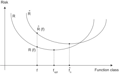
i=1 1 2|f(xi)−yi|, (3.2)

As it is seen, the average value of loss over the training set simply gives the empirical risk. It is crucial to stress that ifFincorporates too many candidate functions or the training set is not large enough, empirical risk minimization paves the way for unsuccessful generalization and high variance. In this case, learning algorithms can just memorize the training examples with a poor generalization which is called over-fitting. IfFis not too large, the increase innwill lead to an approximation of both risk minimizations to each other. It is obvious that the results of the expected and empirical risk minimization are not required to be equal as can be seen in Figure 3.1.

(19)

3.1 SVM: Algorithm Function class Risk f f_opt R R (f) fˆ_n R (f)ˆ Rˆ

Figure 3.1: The minima foptand bfnof the expected (R) and empirical (Rb) risk functions

gener-ally do not coincide. Source: Moro, Hoffmann and Härdle (2010)

fopt=arg min

f∈FR(f), (3.3)

b

fn=arg min

f∈FRb(f), (3.4)

As put before, the other way in statistical learning theory to approximate the distribution of

P(x,y)is calculating the VC bound introduced by Vapnik and Chervonenkis (1971) which rep-resents distribution independent bounds on the generalization performance of a learning ma-chine. Through VC dimension we predict a probabilistic upper bound for the expected risk on the test error of a classification model which holds with a certain probability 1−η. The VC

bound can be written as (Vapnik and Chervonenkis (1971)):

R(f)≤Rb(f) +φ h n, ln(η) n . (3.5)

For a linear indicator functiong(x) =sign(x>w+b):

φ h n, ln(η) n = s h ln2n_h −lnη 4 n , (3.6)

wherehis the VC dimension of the classification model which determines the complexity of a classifier function andnis the size of the training set.hcan be defined as:

h≤min{(r2kwk) +1,n+1} (3.7)

whereris the radius of the smallest sphere composing of data.

(20)

3 Bankruptcy prediction with Support Vector Machines (SVM) -b |w| x o o o o o o o o o o x x x x x x x x x w 0 xT_w+b=0 x 1 x₂ margin d --d+ xT_w+b=1 xT_w+b=-1

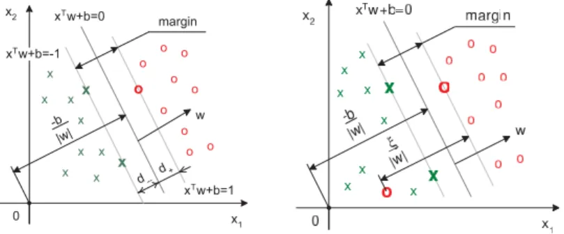
Figure 3.2: The margin in a linearly separable (left) and non-separable (right) case. Crosses and circles are solvent and insolvent companies, respectively. Source: Moro, Hoffmann and Härdle (2010)

function f ∈F can shatter h objects xi∈Rd,i=1, . . . ,h in all 2h possible layouts and no

set

xj∈Rd,j=1, . . . ,q exists whereq>hthat satisfies this property. For instance, suppose

that a straight line is the classification model which has to divide data into two groups and suppose that there are sets of 3 points on a plane (d=2) that can be shattered via this model in 2h=23=8 ways. Nevertheless, in the case of set of 4 points it is not possible to separate one of these two subsets from the other. Thus, the VC dimension of this classifier in a two-dimensional space is three.

Additionally, the functional for the VC bound seen in (3.5) should be further analyzed. Here, VC dimension h is a parameter to control the complexity of the classifier function determin-ing how complicated the classification model can be. Importantly, the second termφ

h n, ln(η) n

represents regularization term introducing a penalty for the excessive complexity of a classifier function. In short, the expected VC-dimension will yield the complexity. Lowerhwill give rise to a larger margin which leads to a good generalization for the future data, but the misclassifi-cation can be higher. Hence, it can be said that there is a trade-off between the misclassifimisclassifi-cation on the training set and the complexity of the classifier function. The SVM aims to construct a model having a minimized VC dimension.(Wang (2005))

The next step in analyzing the SVM is maximizing the margin, the distance of the hyperplane to the closest point in the dataset. This distance shows how well the data is separated. As expected, the wider the margin the clearer is the separation because the ultimate goal is to generalize the separation for the future data as well. Put another way, when the hyperplane is as far away as possible from both of the classes, the generalization is expected to become better. To find the maximum margin we need to solve an optimization problem.

There are two different ways to treat the SVM problem. The first one is the hard margin SVM introduced by Vapnik and Lerner (1963), where the dataset is assumed to be linearly separable by the maximum margin which leads to perfect classification of every data point that can be visualized on the left-hand side in Figure 3.2. However, as mentioned before this is not always the case as seen on the right-hand side of the same figure. Soft margin is developed by Man-gasarian and Bennett (1992) for data being not linearly separable which allows some degree of misclassification of data points.

(21)

3.1 SVM: Algorithm

In the linearly separable case the classification hyperplane of the SVM is:

x>w+b=0, (3.8)

where wis the weight or slope with a dimension of d×1. Here, d will give the number of characteristics of the companies used so as to classify them into solvent and insolvent groups. In this work financial ratios will be used for this purpose. Hence, we haved financial ratios.

xi is a vector of dimensiond×1 representing the financial ratios of companyi. Finally,bis a

scalar that gives the location parameter, the so called threshold.

As put before, when data are linearly separable, the points can be accurately classified with a maximum margin meaning that all observations should satisfy the following constraints:

x>_i w+b≥1 foryi=1,

x>_i w+b≤ −1 foryi=−1,

It is possible to write these two constraints together:

yi(x>i w+b)−1≥0 i=1,2, . . . ,n (3.9)

It is obvious that we have two groups that can be shown as+1(−1). We turn back to the left side of Figure 3.2 again, wherex>_i w+b=±1 are the canonical hyperplanes being parallel to each other. Thend+ (d−) =1/kwkgives the shortest distance between the observations being in the class in question +1(-1) and the separation hyperplane. So the width of the margin is given by 2/kwk. Thus, maximizing the margin means minimizing the Euclidean normkwkor its squarekwk2.

This margin maximization optimization problem can be expressed by a primal Lagrangian as: min wk,b,ξi max αi LP= 1 2kwk 2₋ n

∑

i=1 αi{yi x>_i w+b −1}, (3.10)

whereαiis a Lagrange multiplier.

The Karush-Kuhn-Tucker (KKT) first order optimality conditions are:

∂LP ∂wk =0 ⇐⇒wk− n

∑

i=1 αiyixik=0, k=1, . . . ,d ∂LP ∂b =0 ⇐⇒ n

∑

i=1 αiyi=0 ∂LP ∂ αi =0 ⇐⇒yi x>_i w+b−1≥0 i=1, . . . ,n αi≥0 αi{yi x>_i w+b −1}=0

(22)

whereαi≥0 is the sign condition on the multiplier andαi{yi x>i w+b

−1}=0 represents the complementary slackness.

Then we need to introduce these KKT conditions to the primal problem. We rewrite (3.10) as: 1 2kwk 2₋ n

∑

i=1 αiyix>i w−b n

∑

i=1 αiyi+ n

∑

i=1 αi, We can express n ∑ i=1

αiyix>i wwith the elements of the matrices as:

d

∑

k=1 n

∑

i=1 αiyixikwk (3.11)

As a reminder, d gives the number of financial ratios in this work. Next, we insert wk =

∑nj=1αjyjxjkto (3.11) and get: d

∑

k=1 n

∑

i=1 αiyixik n

∑

j=1 αjyjxjk ! = d

∑

k=1 n

∑

i=1 n

∑

j=1 αiyixikαjyjxjk

Now we can write

d ∑ k=1 n ∑ i=1 n ∑ j=1

xikxjkpart in matrix terms withx>i xj, and what we have becomes: n

∑

i=1 n

∑

j=1 αiαjyiyjx>i xj Importantly, we cancel b n ∑ i=1

αiyi through substituting one of the KKT conditions (Gale and

Tucker (1951)) saying

n

∑

i=1

αiy=0. Finally, we write (3.10) again.

1 2kwk 2₋ n

∑

i=1 n

∑

j=1 αiαjyiyjx>i xj+ n

∑

i=1 αi, (3.12)

We know that the Euclidean norm iskwk=

s d

∑

k=1

w2_k and so we can say that the first term of (3.12) gives the half of the sum of squared weights. Hence, together with the second term which is the sum of the squared weights, the primal problem can be written as the dual problem:

max αi LD= n

∑

i=1 αi− 1 2 n

∑

i=1 n

∑

j=1 αiαjyiyjx>i xj (3.13) s.t.αi≥0, (3.14) n

∑

i=1 αiyi=0. (3.15) 14

(23)

3.1 SVM: Algorithm

It is crucial to note that this optimization problem is convex that both primal and dual problems will yield the same result.

However, as stated before in general this perfectly linearly separation cannot be the case in real life applications where very high dimensional problems are possible. Therefore, it is required now to switch to more general case - linearly non-separable case.

Due to some reasons such as outliers in the dataset it is highly possible to have some data points that fall inside of the margin zone or are on the incorrect side of the margin according to classification. In this situation, it is necessary to have some cost for each misclassification which is determined by how far the data point is from maintaining the margin requirement. Because of this, the inequalities utilized for classification can be rewritten as below which holds for alln

data points of the training set:

x>_i w+b≥1−ξi for yi=1, (3.16)

x>_i w+b≤ −1+ξi for yi=−1, (3.17)

ξi≥0, (3.18)

These three constraints can be expressed by two inequalities which will be used in margin maximization problem: yi x>_i w+b ≥1−ξi (3.19) ξi≥0 (3.20)

where the penalization of misclassification is introduced by ξ being the classification error

depending on the distance from a misclassified pointxito the canonical hyperplane that can be

seen in Figure 3.2 on the right-hand side. Hence, if the value ofξ is greater than zero, it means

that misclassification occurs. As it is seen we allow here for some points to be misclassified but penalize these points appropriately.

With a given training set{(xi,yi)}n_i=1the goal of penalized margin maximization and data

sep-aration can be achieved by solving the following minimization problem of the SVM: min w 1 2kwk 2₊_C n

∑

i=1 ξi, (3.21) subject to yi(x>i w+b)≥1−ξi (3.22) ξi≥0. (3.23)

where the first term in (3.21) is the inverse margin. Thus, through minimizing this term we maximize the margin. In the second part of the problem,Creflects how good the used algorithm will be in classifying unlabeled future data; in other words,Cis the complexity. As the value of

Cgets smaller, the margin will widen and this parameter provides us with a way to control for the over-fitting problem. However, the smallerCmay lead to higher degree of misclassification, as mentioned before. Besides,

n

∑

i=1

(24)

Now we can proceed to primal Lagrange functional: min w,b,ξi max αi,µi LP= 1 2kwk 2₊ C n

∑

i=1 ξi− n

∑

i=1 αi{yi x>_i w+b −1+ξi} − n

∑

i=1 µiξi, (3.24)

whereαi≥0 andµi≥0 are Lagrange multipliers.

KKT first order optimality conditions are:

∂LP ∂wk =0 ⇐⇒wk− n

∑

i=1 αiyixik=0, k=1, . . . ,d ∂LP ∂b =0 ⇐⇒ n

∑

i=1 αiyi=0 ∂LP ∂ αi =0 ⇐⇒yi x>_i w+b −1+ξi≥0 i=1, . . . ,n ∂LP ∂ µi =0 ⇐⇒ξi≥0 i=1, . . . ,n αi≥0 µi≥0 αi{yi x_i>w+b −1+ξi}=0 µiξi=0

After we substitute the KKT conditions into the primal problem, we get the dual Lagrangian: max αi LD= n

∑

i=1 αi− 1 2 n

∑

i=1 n

∑

j=1 αiαjyiyjx>i xj, (3.25) s.t. 0≤αi≤C, (3.26) n

∑

i=1 αiyi=0. (3.27)

So far the hyperplane we are searching for is a linear classifier. However, we know that it is also possible to use SVMs as nonlinear classifiers via the classic kernel trick which enables to embed the data pointsxi into a higher dimensional Hilbert space. This trick is possible because of the

fact that all the training vectors in the dual problem are expressed as scalar products,x>_i xj. This

mapping can be shown as:

Φ:Rd7→H

What we will do is to seek a linear classifier in the feature spaceH, which is in fact nonlinear

in the original space R. It is worth stressing that thanks to this kernel trick it is possible to

utilize any kernel matrix K defined by K(xi,xj) =Φ(xi)Φ(xj) without knowing exactly the

high dimensional mapping Φ. In a simple way, instead of using x>i xj in order to solve the

learning problem, we transfer all the data to a higher dimensional space through replacingx>_i xj

byK(xi,xj). According to Mercer’s theorem Martin (1909) any positive semi-definite matrix is

a valid kernel matrix meaning that for any dataset x1, . . . ,xn and any real numbersϒ1, . . . ,ϒn,

(25)

3.1 SVM: Algorithm

the functionKshould verify

n

∑

i=1 n

∑

j=1 ϒiϒj≥0 (3.28)

In this work, as mentioned before Gaussian RBF will be applied:

K(xi,xj) =exp{− xi−xj

/(2r2)} (3.29)

whereris the radial bases giving the minimum radius of a data group.

After solving the dual SVM problem, we will find Lagrange multipliersα which take the value

of zero for non-support vectors. Support vectors are the training points which are not classified clearly, so that they are either misclassified, or are correctly classified but lie in the margin zone. Accordingly, theαivalues of support vectors will depict non-zero values. As a result, it can be

noted that the higher theαi, the more difficult it is for an observation to be assigned to a class.

After deriving Lagrange multipliers, with the help of the linear relationship we will get the slope of the separating functionw:

w=

n

∑

i=1

αiyixi (3.30)

With the acquired values ofw, the next step will be the separation of companies into two groups, namely "solvent" and "insolvent" through using the classification rule given by (3.31). However, this is the case when it is possible to classify data linearly in the original spaceR.

g(x) =sign

x>w+b

, (3.31)

In (3.31) the threshold parameter isb= 1₂(x+1+x−1)w. x+1 andx−1are two support vectors

belonging to different classes lying on the margin boundary. The use of averages over allx₊and

x−instead of two arbitrarily chosen support vectors is preferable in order to mitigate numerical errors while training the SVM (Moro et al. (2010)). Furthermore, in the linearly separable case, scores of each company can be calculated as:

f(x) =x>w+b. (3.32)

Nevertheless, in this work we are interested in the more general case where data is linearly nonseparable in R. In such a case, we have a linear classifier gN(x) in the feature space H

shown as: gN(x) =sign n

∑

i=1 yiαiK(xi,xj) +b ! , (3.33)

and the scores of a companies are given by:

f(x) =

n

∑

i=1

(26)

Next how we can solve this classification problem is important. Due to the fact that the optimiza-tion problem in quesoptimiza-tion is a quadratic one it is possible to solve it by the means of quadratic programming (QP); nonetheless, there are significant problems:

1. solving the problem is extremely time consuming 2. it requires a huge memory

To overcome these problems while solving the optimization problem three possible methods can be succinctly introduced. Firstly, the Chunking algorithm developed by Vapnik (1979) can be shown to be an effective method for decreasing the required time and reducing the huge memory requirement while optimizing the SVM in relation to the classical QP optimization. This method uses support vectors having non-zero Lagrange multipliers (α 6=0) to solve the problem and

ignores the other observations. Thus, thanks to this method we can maintain a reduced training set and simplify the optimization problem. It is clear that this algorithm depends on the idea that the solution of QP optimization will not be changed if we disregard vectors withα =0.

The steps of the general chunking procedure can be described as:

1. Decompose the original dataset as: training dataset and testing dataset. 2. Optimize the reduced training set by classical QP optimization. 3. Obtain the support vectors by the previous optimization. 4. Test the support vectors in testing dataset.

5. Recombine support vectors and testing errors on a new training set. 6. Repeat from step 2 until errors are reduced enough by 4.

The other method is developed by Osuna and F. (1997) in which the number of observations is not reduced, but instead it is kept constant. The idea is that after solving the QP problem, one of the observations is replaced with the one that contradicts with the KKT optimality conditions. Both of the mentioned methods utilize the QP solver. Additionally, another method, namely Sequential Minimal Optimization, was introduced by Platt (1998) which solves the relevant optimization problem analytically. In this work, chunking method will be applied.

After solving the dual problem and predicting scores f(x)through learning algorithm, we will find the probability of default (PD) for each company. The PD is a conditional probability which can be defined as the probability ofY =1 givenX=x. The PD of a company gives the likelihood that the company will not repay its loan, in other words it will default on the loan. Let’s define this conditional probability as:

η(x) =P(Y =1|X=x) ∀x∈X, η(x)∈[0,1]

In this work, through using least square loss function we get the following formula to calculate PDs from each value of company scores f(x).

b

η(x) = f(xi) +1

2 (3.35)

All in all, in predicting company failures with the SVM we have two phases, namely training and test phases. During the training phase, the SVM estimates weightswof the financial ratios, and

(27)

3.1 SVM: Algorithm

through doing this it learns the mappingy= f(x,w)that is done by the system. What we look for is an approximating function fa(x,w)∼ythat can have a good generalization performance

on the future data. Following training, we have test phase, where we expect that the output from a machineo=fa(x,w)is a good estimate of the true responsey.

(28)

(29)

4 Bankruptcy prediction with logistic

regression

The other possible method to predict corporate failure by using financial ratiosXjis the logistic

model. In this model, it is assumed that(X₁,Y₁), . . . ,(Xn,Yn)is an independently and identically

distributed random sample, whereXj ∈Rd. The dependent variableYj is a Bernoulli random

variable taking the value of 1 and 0 referring to bankrupt and non-bankrupt companies in this work, respectively.

Through using logistic regression we will try to fit data to a logit function to predict the PD given some financial ratios P(Yj=1|Xj=x). Because of the fact that the regression is binomial,

the generalized linear model (GLM), which was introduced by Nelder and Wedderburn (1972), will be utilized. We can not predict default probability through using a linear regression of

β0+β>X because here, there is no guarantee that the probability will lie between the values

of 0 and 1. Therefore, GLM will be used to predict the probability. The scores are computed byβ0+β>X meaning that they are linear combinations of the relevant financial ratios. After

calculating the scores, the probabilities of default will be estimated with a link functionG:

φ(X) =P(Yj=1|Xj=x) =G(β0+β>X) (4.1)

whereG:R→[0,1]is a known function which is selected as logistic here taking the values

between 0 and 1:

G(s) =γ(s) = 1

1+e−s (4.2)

wheresgives scores. Hence, scores can also be written as the log of odds:

s=ln γ(s) 1−γ(s) (4.3)

The real values ofβ0, . . . ,βd are not known and required to be estimated. The maximum

like-lihood procedure will be applied to estimate them. The conditional likelike-lihood function can be written as: L(β0, . . . ,βd) = n

∏

j=1 [Yjγ(β0+β>Xj) + (1−Yj){1−γ(β0+β>Xj)}] (4.4)

(30)

log-4 Bankruptcy prediction with logistic regression

likelihood function can be written as: logL(β0, . . . ,βd) =

n

∑

j=1

[Yjlogγ(β0+β>Xj) + (1−Yj)log{1−γ(β0+β>Xj)}] (4.5)

Then,Lor logLis maximized to get the maximum estimators_βb₀, . . . ,_βb_dof_β₀, . . . ,_β_dand lastly,

we obtain the maximum likelihood estimator for the PD (Franke and Hafner (2004)):

b

φ(X) =γ(_βb₀+_βb₀

>

X) (4.6)

Next, it is essential to explain which financial ratios should be added to the model to predict default probabilities in a most accurate way. To select the best model, we will check one of the measures of the goodness of fit, namely Akaike’s information criterion (AIC) proposed in Akaike (1974). Through using backward stepwise regression, the analysis will start with all financial ratios and the ratios will be eliminated from the model sequentially. In each step of elimination, theAIC will be calculated. Then, these models are ranked according to theirAIC

and the model having the lowestAICwill be selected. TheAICcan be calculated as:

AIC=−2 logL+2p (4.7)

where Lis the maximized log likelihood of the model fit and prepresents the number of es-timated parameters. The model having a good fit to data has a low value of deviance statistic −2 logL. Furthermore, 2pis added to the AIC to penalize the likelihood for each parameter added to the model because addition of the parameters makes the model more complicated. After selecting the model with lowest AIC, chi-square test is applied to prove how well the chosen logistic regression model fits the data. To calculate the chi-square statistic, the difference in deviance statistics for the final model and the null model, a model with just an intercept , will be taken. In other words, to get the required test statistic the difference between the maximized value of the likelihood functions for the null modelLN and the final modelLF should be found

which can be expressed as:

χ2= (−2 logLN)−(−2 logLF) (4.8)

The degrees of freedom is equal to the number of parameters in the final model.

In the last step, to compare the goodness of fit of logistic and SVM models, the Lorenz curve will be plotted which was introduced by Lorenz (1905). With the help of this graph accuracy of scoresswith respect to their predictive power for a company default is visualized for both mod-els. Simply put, the Lorenz curve is a plot of P(S<s)against P(S<s|Yj =1). Thus, it is clear

that the aim is to understand which of the models classifies more companies as "non-bankrupt" depending on their own dataset, although they went "bankrupt" in reality. And according to the visualization of the level of this misclassification we try to assess the performances of logistic and SVM models and decide which model outperforms the other.

(31)

5 Data description

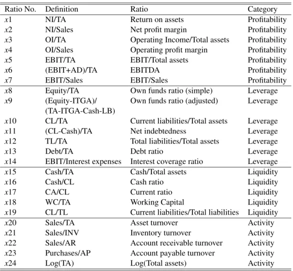
The dataset consists of 20000 solvent and 1000 insolvent German companies. It is obtained from the Credit reform database provided by the Research Data Center (RDC). The analyzed period runs from 1996 to 2002 and it is important to stress that the information regarding insolvent companies is acquired 2 years before the insolvency occurred. The label variabley takes the value of−1 for solvent companies and 1 for the last report of a company before its insolvency. We have 28 financial variables belonging to the companies. The variables are such as cash, earnings before interest and taxes (EBIT), amortization and depreciation (AD), intangible assets (ITGA) and lands and buildings (LB). Through using these variables 24 financial ratios are computed which are put into four groups so called profitability, leverage, liquidity, and activity shown in Table 5.1.

5.1 Data cleaning and model selection

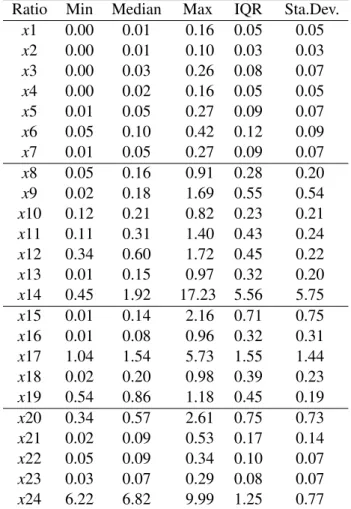
The SVM is sensitive to outliers, because outlier points play the most important role in de-termining the decision hyperplane. To enhance the SVM the effect of outliers are decreased through equalizing the data points greater than the upper outlier to this upper value and simi-larly replacing the values smaller than the lower outlier by this lower value. Upper and lower limits are calculated byQ75+1.5∗IQandQ25−1.5∗IQ, respectively where Q represents the quantile. Besides, it is required to note that in the year of 1996 we have just insolvent companies so that the data of this year will not be incorporated to the calculations. Descriptive statistics of financial ratios are given in Table 5.2.

The next and very important step is to select the most powerful financial ratios in separating the companies into two groups; solvent and insolvent. In this work, backward and forward stepwise selection techniques are utilized in MATLAB 7.0 and then the results are compared to show how important it is to decide which financial ratios should be incorporated to the SVM model. Due to the fact that we have too many financial ratios, the critical value is taken as 0.01 in both techniques to receive the most important ones and eliminate others.

In the case of backward stepwise selection, the procedure starts with all variables, and the variables having less significance according to the chosen critical level are then sequentially removed. This procedure will continue until all remaining variables are statistically significant. After the application of this method, the model comprisingx1,x3,x5,x6,x8,x11,x13,x18 and

x24 is chosen. The selection of the financial ratios poses a meaningful picture, since with this selection the model has at least one financial ratio from each category seen in Table 5.3. At this point, it is required to mention the importance of the selected financial ratios. The return on assets defines how profitable a company’s assets are in terms of generating revenues. Thus, it shows how efficiently a company can convert its assets into net income. Therefore, using this ratio in separation of companies seems highly reasonable. Additionally, other chosen

(32)

5 Data description

Ratio No. Definition Ratio Category

x1 NI/TA Return on assets Profitability

x2 NI/Sales Net profit margin Profitability

x3 OI/TA Operating Income/Total assets Profitability

x4 OI/Sales Operating profit margin Profitability

x5 EBIT/TA EBIT/Total assets Profitability

x6 (EBIT+AD)/TA EBITDA Profitability

x7 EBIT/Sales EBIT/Sales Profitability

x8 Equity/TA Own funds ratio (simple) Leverage

x9 (Equity-ITGA)/ Own funds ratio (adjusted) Leverage

(TA-ITGA-Cash-LB)

x10 CL/TA Current liabilities/Total assets Leverage

x11 (CL-Cash)/TA Net indebtedness Leverage

x12 TL/TA Total liabilities/Total assets Leverage

x13 Debt/TA Debt ratio Leverage

x14 EBIT/Interest expenses Interest coverage ratio Leverage

x15 Cash/TA Cash/Total assets Liquidity

x16 Cash/CL Cash ratio Liquidity

x17 CA/CL Current ratio Liquidity

x18 WC/TA Working Capital Liquidity

x19 CL/TL Current liabilities/Total liabilities Liquidity

x20 Sales/TA Asset turnover Activity

x21 Sales/INV Inventory turnover Activity

x22 Sales/AR Account receivable turnover Activity

x23 Purchases/AP Account payable turnover Activity

x24 Log(TA) Log(Total assets) Activity

Table 5.1: Definitions of financial ratios.

(33)

5.1 Data cleaning and model selection

Ratio Min Median Max IQR Sta.Dev.

x1 0.00 0.01 0.16 0.05 0.05 x2 0.00 0.01 0.10 0.03 0.03 x3 0.00 0.03 0.26 0.08 0.07 x4 0.00 0.02 0.16 0.05 0.05 x5 0.01 0.05 0.27 0.09 0.07 x6 0.05 0.10 0.42 0.12 0.09 x7 0.01 0.05 0.27 0.09 0.07 x8 0.05 0.16 0.91 0.28 0.20 x9 0.02 0.18 1.69 0.55 0.54 x10 0.12 0.21 0.82 0.23 0.21 x11 0.11 0.31 1.40 0.43 0.24 x12 0.34 0.60 1.72 0.45 0.22 x13 0.01 0.15 0.97 0.32 0.20 x14 0.45 1.92 17.23 5.56 5.75 x15 0.01 0.14 2.16 0.71 0.75 x16 0.01 0.08 0.96 0.32 0.31 x17 1.04 1.54 5.73 1.55 1.44 x18 0.02 0.20 0.98 0.39 0.23 x19 0.54 0.86 1.18 0.45 0.19 x20 0.34 0.57 2.61 0.75 0.73 x21 0.02 0.09 0.53 0.17 0.14 x22 0.05 0.09 0.34 0.10 0.07 x23 0.03 0.07 0.29 0.08 0.07 x24 6.22 6.82 9.99 1.25 0.77

Table 5.2: Descriptive statistics for financial ratios. IQR is the interquartile range. Descriptive

x11 (CL-Cash)/TA Net indebtedness Leverage

x13 Debt/TA Debt ratio Leverage

x18 WC/TA Working Capital Liquidity

Table 5.3: The selected financial ratios via backward stepwise method to be used in the SVM model. SVMbackward

(34)

5 Data description

profitability financial ratios, EBIT/Sales and (EBIT+DA)/TA, are again the measures of the efficiency of a company in generating returns from its assets. In the calculation of second financial ratio depreciation and amortization are added to EBIT, since they are not counted as operating expenses. The other significant financial ratio in the same category is operating profit margin which reflects the strength of the company in paying its fixed costs, such as interest and debt. All in all, it can be said that the higher these profitability ratios, the lower is the company’s financial risk. As to the leverage category, own funds ratio (simple), net indebtedness and debt ratio are selected via backward stepwise selection. Own funds ratio tells us the solvency level of a company through giving its ability to raise money to remain viable. Net indebtedness reflects a company’s debt situation after subtracting its cash from the value of its liabilities. Debt ratio provides similar information. Through looking at debt ratio it is possible to grasp the ability of a company to secure its financing. Hence, the selected leverage financial ratios are important variables for assessing the ability of a company to sustain risk. In liquidity category the ratio of working capital to total assets is chosen where working capital is given by current assets; thus, the relevant ratio gives the amount of operating capital of the company that can be used for growth or acquisitions. When this ratio has a positive sign, it means that the company has adequate funds to meet its operational expenses and short-term debt. Lastly, for the category of activity, log of total assets will be used which is the log of the size of the company. A company’s size can be seen as a risk factor for bankruptcy. It is mostly believed that large companies are unlikely to go bankrupt. However, there are some instances of bankrupted huge enterprises in real life that contradict this claim, such as Enron, Barings Bank, and Worldcom. Hence, we can not have an exact comment on the effect of company size on the company default risk.

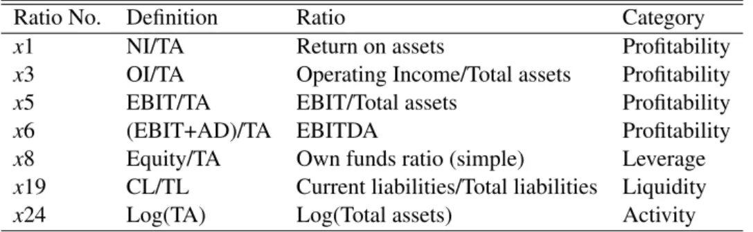
As to the other technique of variable selection, forward stepwise selection, the procedure starts with an intercept model and then proceeds through adding financial ratios sequentially to the model and stop when no additional financial ratio can improve the fit significantly. According to this methodx1,x3,x5,x6,x8,x19 andx24 are chosen, and again we have at least one variable relating to each category of financial ratios as represented in Table 5.4. Compared to backward stepwise selection method we have fewer amounts of variables, but six of them are common after using both techniques. Here, the only different financial ratio from those selected by backward technique is the ratio of current liabilities to total liabilities which is in the liquidity category. Current liabilities are all debts or obligations of the company due within twelve months; thus, it is an important measure which provides information regarding the company’s liquidity position. Hence, this ratio can been as a crucial measure reflecting the company’s debt structure and so gives an aspect of a company’s financial performance as well. All in all, including this ratio to the SVM model seems reasonable.

(35)

5.1 Data cleaning and model selection

x19 CL/TL Current liabilities/Total liabilities Liquidity

Table 5.4: The selected financial ratios via forward stepwise method to be used in the SVM model. SVMforward

(36)

(37)

6 Empirical Results

6.1 Results on the SVM model

In this part, the aim is to calculate the score values, then the PDs for each company and lastly, to obtain the classification of two groups of bankrupt and non-bankrupt companies. It is known that after the selection of variables the result of the margin maximization problem which gives the effectiveness of the SVM in classification depends heavily on the values ofC, the capacity, andr, the kernel’s parameter. As mentioned before, r is the minimum radius containing the data. Additionally, the selection of kernel is critically important in determining how good the separation can be. As stated earlier, Gaussian RBF is applied in this work. The optimization problem of the SVM model is solved with MATLAB 7.0.

For the model with the 9 financial ratios found by using backward stepwise selection, a train-ing set and test set are taken in a 2 : 1 ratio. In the traintrain-ing set there are randomly selected 100 solvent and 100 insolvent companies, whereas in the test set we have 50 companies for each group. It is observed that increasing the number of companies in the training set wors-ens the performance of the SVM model as a classifier. Through changing the values ofCand

r we get different performances given by the accuracy ratio (AR). At this point, it is crucial to find the best combination of C and r which gives the highest AR. To achieve this result grid-search with exponentially growing sequences of these two relevant parameters is applied, whereC∈ {2−5,2−3, . . . ,213,215}andr∈ {2−15,2−13, . . . ,21,23}. Through using cross valida-tion each possible pair of parameters is checked and then the parameters giving the highest cross validation accuracy are selected. The highest AR of 72% is obtained byC=16 andr=2. The AR results of other combinations of the parameters can be seen in Table 6.1. Next, we check what will happen when included information is decreased. For example, net indebtedness ratio is dropped and after applying cross validation to the model with 8 financial ratios the highest AR of 75% is achieved withC=128 andr=4, the visualization of which can be seen in Figure 6.1 derived in R 2.12.0. As mentioned before, we found the PDs from company scores through using least square loss function and because of the fact that what we found is just the estimates of the probabilities some values are outside the interval{0,1}. To solve this problem the values higher than one are set equal to one and the values smaller than zero are set equal to zero. To conclude, although a statistical method is used to select the best financial ratios, we see that dropping a financial ratio can improve the model’s performance. Thus, incorporating too much information to the model does not necessarily lead to improvement of the model. It is obvious that it is not easy to find the model with the highest AR.

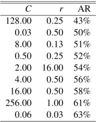
As to the model with 7 financial ratios based on forward stepwise selection, we use the same training and test sets and we apply cross validation method depending on the same intervals used previously for the parameters ofCandr. In this case, AR posted the best value at 64% withC=256 andr=2. It is observed that using different financial ratios based on different variable selection procedures affects the performance of the SVM model significantly. How the

(38)

6 Empirical Results ● ●● ●● ● ●● ● ●● ●● ● ● ●●●● ●●●● ● ● ● ● ● ●●●● ●●●● ●●●● ●●●●● ●● ● ● ● ● ● ● ● ● ● ● ● ● ● ●●●●●●●●●●●●●●●●●●●●● ●●● ●●●●●● ●●●●●● ● ● ● ● −1 0 1 2 3 0.0 0.2 0.4 0.6 0.8 1.0 Probability of Default (SVM) scores Y

Figure 6.1: The SVM model with AR=75% where the blue line represents the PDs of the com-panies and red dots are the scores. SVMpd

C r AR 16.00 0.06 49% 0.03 8.00 50% 0.50 4.00 53% 0.25 1.00 55% 0.25 0.25 57% 16.00 0.25 58% 2.00 1.00 59% 0.50 0.50 60% 4.00 1.00 65% 8.00 1.00 68%

Table 6.1: The effect of different pairs ofCandr on AR of the SVM model composed of the financial ratios given by backward selection method. SVMcrbackward

(39)

6.1 Results on the SVM model C r AR 128.00 0.25 43% 0.03 0.50 50% 8.00 0.13 51% 0.50 0.25 52% 2.00 16.00 54% 4.00 0.50 56% 16.00 0.50 58% 256.00 1.00 61% 0.06 0.03 63%

Table 6.2: The effect of different pairs ofCandron AR of the SVM model composed of the financial ratios given by forward selection method. SVMcrforward

different combinations of parameters influence the values of AR can be observed in Table 6.2. To visualize how the effectiveness of the SVM classification varies according to the parameters ofCandr, different instances will be analyzed in two dimensions through using the model with

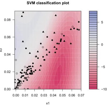
x1 andx3 consisting of randomly chosen 100 solvent 100 insolvent companies. The graphs are produced with R 2.12.0. As a reminder,x1 andx3 refer to return on assets and the ratio of operating income to total assets, respectively both of which belong to the profitability group. Intonation of the related figures depends on the level of scores f. As it is known, the higher the scores, the higher is the PD of the company. When the score value gets larger, the color should become blue; in other words, the more blue color represents the higher score value and in parallel the higher PD. As to the areas with companies having low or negative scores, the color should get more red. Thus, the regions of the graph filled with successful companies are expected to be red in the case of a good classification. Additionally, triangles and circles are solvent and insolvent companies, respectively and the ones which are filled with black color represent the support vectors.

Firstly, we will check how the performance of the SVM changes according to the different values ofr. In Figure 6.2 the values of the parameters areC=100 andr=1. In this case, it can obviously be seen that there is no successful classification. The reason might be thatCremains too high according to the value ofr. Then, we increase the value of rto 8 while keeping the value ofCinvariant and SVM starts to classify the companies given in Figure 6.3. As it is seen, blue areas are filled with insolvent companies and red ones with solvent companies. Next, r

is increased to 100 while keepingC constant presented in Figure 6.4 so as to figure out what happens whenrtakes a very high value. It can be observed that the colorful areas become very small and unclear meaning that we increase the minimum radiusrto an undesirable high level. There are some correct classifications on the left bottom, though.

It is already stated that the capacityChas an inverse relationship with the width of the margin. The analysis of the impact of the changes inCon the classification performance of SVM will be performed while keeping the value ofrat 8 in each case. Firstly, the value ofCis taken as 0.1 in Figure 6.5. As it is seen, almost all of the companies become support vectors, although SVM recognizes the few successful companies on the left bottom side of the figure. It is obvious that the value ofC needs to be raised. In Figure 6.6, we increase the value ofC slightly to 0.5 to observe how sensitive the SVM is to the capacity parameter, and the result changes

(40)

6 Empirical Results −10 −5 0 5 0.00 0.01 0.02 0.03 0.04 0.05 0.06 0.07 0.00 0.02 0.04 0.06 0.08 ● ● ● ● ● ● ● ● ● ● ● ● ● ● ● ● ● ● ● ● ● ● ● ● ● ● ● ● ● ● ● ● ● ● ● ● ● ● ● ● ● ● ● ● ● ● ● ● ● ● ● ● ● ● ● ● ● ● ● ● ● ● ● ● ● ● ● ● ● ● ● ● ● SVM classification plot x1 x3

Figure 6.2: Assessment of the SVM classification performance in two dimensions whereC=

100 andr=1. SVMc100r1 −5 0 5 0.00 0.01 0.02 0.03 0.04 0.05 0.06 0.07 0.00 0.02 0.04 0.06 0.08 _● ● ● ● ● ● ● ● ● ● ● ● ● ● ● ● ● ● ● ● ● ● ● ● ● ● ● ● ● ● ● ● ● ● ● ● ● ● ● ● ● ● ● ● ● ● ● ● ● ● ● ● ● ● ● ● ● ● ● ● ● ● ● ● ● ● ● ● ● ● ● ● ● SVM classification plot x1 x3

100 andr=8. SVMc100r8

(41)

6.2 Results on logistic regression −8 −6 −4 −2 0 2 4 6 0.00 0.01 0.02 0.03 0.04 0.05 0.06 0.07 0.00 0.02 0.04 0.06 0.08 ● ● ● ● ● ● ● ● ● ● ● ● ● ● ● ● ● ● ● ● ● ● ● ● ● ● ● ● ● ● ● ● ● ● ● ● ● ● ● ● ● ● ● ● ● ● ● ● ● ● ● ● ● ● ● ● ● ● ● ● ● ● ● ● ● ● ● ● ● ● ● SVM classification plot x1 x3

100 andr=100. SVMc100r100

considerably with blue and red clusters being full with correct companies and the number of support vectors decreases as well. Next, in Figure 6.7, the parameters areC=170 and r=8 and it is observed that the groups are separated with blue and red regions, whereas Figure 6.8 derived with the parameters ofC=10000 andr=8 indicates that with very high values ofCthe distance between two groups of companies gets very narrow that SVM starts not to recognize the bankrupt companies yielding unsuccessful classification.

After analyzing the crucial effect of the selection of C and r on the SVM’s performance, it becomes clearer that a statistical method should be applied in order to find the optimum pair of parameters giving the best SVM classification on data.

6.2 Results on logistic regression

In this section, the results of logistic regression model will be given. The data includes 500 solvent and 500 insolvent companies randomly chosen from the same dataset provided by RDC. As mentioned before, the response variableY∈ {0,1}is binary and the value of−1 used before for the solvent companies is changed with 0 here and we leave the value of 1 for the insolvent companies unchanged.

To choose the best model with the given financial ratios theAICstepwise algorithm is applied. We adopt backward elimination, where the procedure starts with all financial ratios. Then, financial ratios are removed sequentially and theAICis computed at each step. As put before, among the candidate models, the model with the lowestAICis desirable. TheAICtouched the lowest value at 1164.92 which gives the final model composed ofx1, x3, x12, x15, x16, x18,

(42)

6 Empirical Results −1.0 −0.5 0.0 0.5 1.0 0.00 0.01 0.02 0.03 0.04 0.05 0.06 0.07 0.00 0.02 0.04 0.06 0.08 _● ● ● ● ● ● ● ● ● ● ● ● ● ● ● ● ● ● ● ● ● ● ● ● ● ● ● ● ● ● ● ● ● ● ● ● ● ● ● ● ● ● ● ● ● ● ● ● ● ● ● ● ● ● ● ● ● ● ● ● ● ● ● ● ● ● ● ● ● ● ● SVM classification plot x1 x3

0.1 andr=8. SVMc01r8 −1.0 −0.5 0.0 0.5 1.0 1.5 0.00 0.01 0.02 0.03 0.04 0.05 0.06 0.07 0.00 0.02 0.04 0.06 0.08 _● ● ● ● ● ● ● ● ● ● ● ● ● ● ● ● ● ● ● ● ● ● ● ● ● ● ● ● ● ● ● ● ● ● ● ● ● ● ● ● ● ● ● ● ● ● ● ● ● ● ● ● ● ● ● ● ● ● ●_● ● ● ● ● ● ● ● ● ● ● ● ● SVM classification plot x1 x3

0.5 andr=8. SVMc05r8

(43)

6.2 Results on logistic regression −10 −5 0 5 10 0.00 0.01 0.02 0.03 0.04 0.05 0.06 0.07 0.00 0.02 0.04 0.06 0.08 ● ● ● ● ● ● ● ● ● ● ● ● ● ● ● ● ● ● ● ● ● ● ● ● ● ● ● ● ● ● ● ● ● ● ● ● ● ● ● ● ● ● ● ● ● ● ● ● ● ● ● ● ● ● ● ● ● ● ● ● ● ● ● ● ● ● ● ● ● ● ● ● ● SVM classification plot x1 x3

170 andr=8. SVMc170r8 −40 −30 −20 −10 0 10 0.00 0.01 0.02 0.03 0.04 0.05 0.06 0.07 0.00 0.02 0.04 0.06 0.08 ● ● ● ● ● ● ● ● ● ● ● ● ● ● ● ● ● ●_● ● ● ● ● ● ● ● ● ● ● ● ● ● ● ● ● ● ● ● ● ● ● ● ● ● ● ● ● ● ● ● ● ● ● ● ● ● ● ● ● ● ● ● ● ● ● ● ● ● ● ● ● ● ● ● ● SVM classification plot x1 x3

Bankruptcy prediction with support vector machines