Spatio-temporal forecasting of network data

(1)

1

Spatio-temporal forecasting of

network data

James Haworth

Department of Civil, Environmental and Geomatic Engineering,

University College London

Supervisors: Prof. Tao Cheng Prof. John Shawe-Taylor

A thesis sumbitted in partial fulfilment of the requirements for the

degree of

Doctor of Philosophy in Geographic Information Science

(2)

2

Statement of Originality

I, James Haworth confirm that the work presented in this thesis is my own. Where information has been derived from other sources, I confirm that this has been indicated in

the thesis.

Signed: Date:

(3)

3

Abstract

In the digital age, data are collected in unprecedented volumes on a plethora of networks. These data provide opportunities to develop our understanding of network processes by allowing data to drive method, revealing new and often unexpected insights. To date, there has been extensive research into the structure and function of complex networks, but there is scope for improvement in modelling the spatio-temporal evolution of network processes in order to forecast future conditions.

This thesis focusses on forecasting using data collected on road networks. Road traffic congestion is a serious and persistent problem in most major cities around the world, and it is the task of researchers and traffic engineers to make use of voluminous traffic data to help alleviate congestion. Recently, spatio-temporal models have been applied to traffic data, showing improvements over time series methods. Although progress has been made, challenges remain. Firstly, most existing methods perform well under typical conditions, but less well under atypical conditions. Secondly, existing spatio-temporal models have been applied to traffic data with high spatial resolution, and there has been little research into how to incorporate spatial information on spatially sparse sensor networks, where the dependency relationships between locations are uncertain. Thirdly, traffic data is characterised by high missing rates, and existing methods are generally poorly equipped to deal with this in a real time setting.

In this thesis, a local online kernel ridge regression model is developed that addresses these three issues, with application to forecasting of travel times collected by automatic number plate recognition on London’s road network. The model parameters can vary spatially and temporally, allowing it to better model the time varying characteristics of traffic data, and to deal with abnormal traffic situations. Methods are defined for linking the spatially sparse sensor network to the physical road network, providing an improved representation of the spatial relationship between sensor locations. The incorporation of the spatio-temporal neighbourhood enables the model to forecast effectively under missing data. The proposed model outperforms a range of benchmark models at forecasting under normal conditions, and under various missing data scenarios.

(4)

4

Acknowledgements

This thesis would not have been possible without the fantastic support of the people around me. First and foremost, I thank my supervisor, Prof. Tao Cheng. Throughout the past 4 (and a bit) years she been unwavering in her support, and has given up a huge amount of her time helping me to make the best of my research. She has always believed in my ideas and provided me with the motivation to continue, helping me through the more difficult times and joining in the better times. I also thank my second supervisor, Prof. John Shawe-Taylor, for his valuable contribution to my work. Spending one hour talking with him is worth a month or more buried in books.

I also owe a debt of gratitude to the members of the STANDARD project; Andy Emmonds, Jonathan Turner and Alex Santacreu at Transport for London; and Prof. Benjamin Heydecker and Dr. Andy Chow at UCL. Your experience and knowledge cannot be matched, and has been invaluable to me.

I would also be nowhere without the support, advice and friendliness of my colleagues at UCL. Jiaqiu Wang helped me find my feet when I was new to the PhD life, and I have enjoyed collaborating with him over the past four years immensely. My friends at UCL, Ed Manley, Adel Bolbol, Garavig Tanaksaranond, Berk Anbaroglu, Ioannis Tsapakis, Jingxin Dong, Monsuru Adepeju, Leto Peel, Suzy Moat and Ryan Davenport have helped make these some of the most enjoyable years of my life, despite the challenges we have all faced together. I also thank the Engineering and Physical Sciences Research Council (Grant EP/G023212/1) for their financial support, and Transport for London for providing the data used in this thesis.

Finally, I thank my family and friends outside of UCL, especially my parents, Christine and Malcolm, for putting a roof over my head for the first three years of my PhD (and many before), and Amy, for putting up with a PhD student for so long, which is no easy task. The fact they all remember who I am after the past year shows what caring people they all are.

(5)

5

List of Figures

1.1 – Thesis roadmap 19

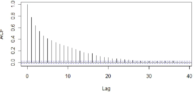
2.1 – A typical ACF plot showing strong, significant autocorrelation, decaying exponentially toward zero

29 2.2 – Comparison of nature, statistical models and machine learning 34

2.3- The concept of overfitting and underfitting 35

3.1 – The macroscopic fundamental diagram 47

4.1 – Observing travel times using ANPR 93

4.2 – Example of journey time data collected on the LCAP network 95

4.3 – The ITN and LCAP Networks 96

4.4 - Closer view of spatial coverage of LCAP within CCZ 97

4.5– Histogram of link lengths 98

4.6 – Link lengths on the LCAP network 99

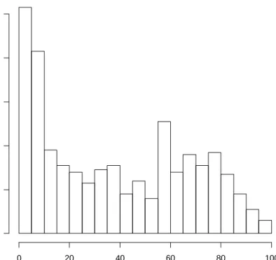
4.7 – Histogram of frequency of observation 102

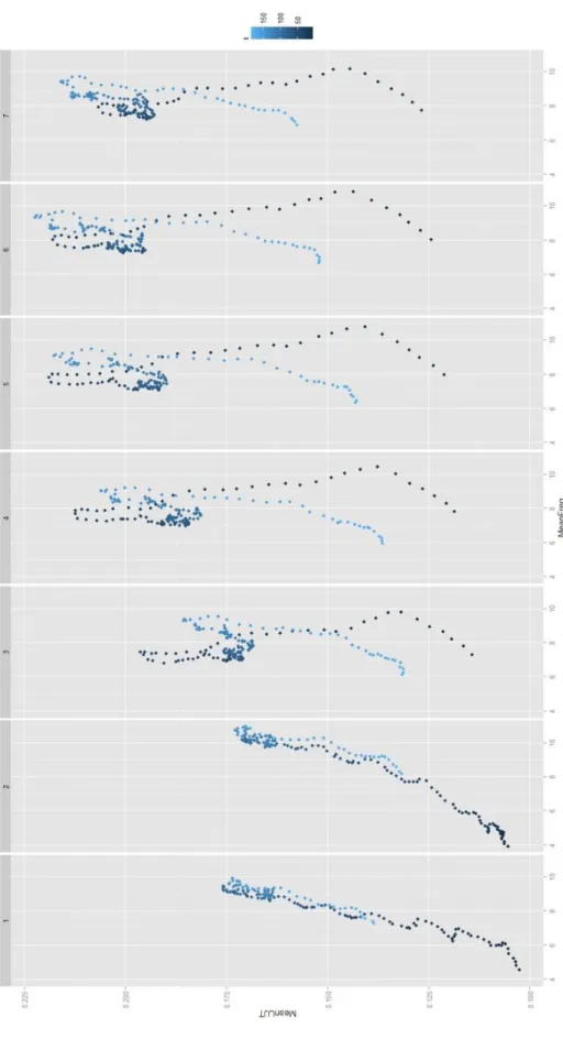
4.8 – Profile of mean frequency of observation across the week 103 4.9 – Relationship between mean frequency and mean journey time across the test

network.

104 4.10 – Histogram of missing data percentages on the LCAP network 107

4.11 – Average Patch types across the week 107

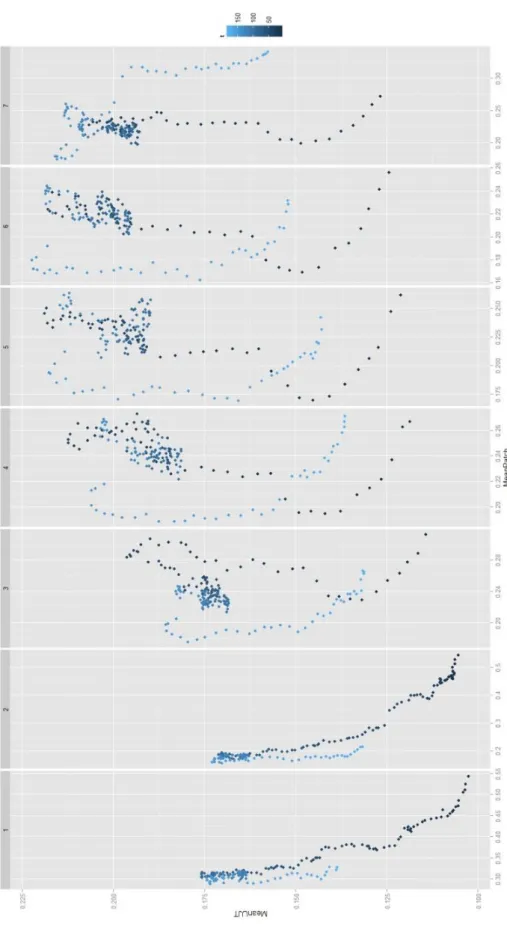
4.12 - Relationship between mean patch type and mean journey time across the test network.

108

4.13 – Extent of the LCAP Network after data cleaning 111

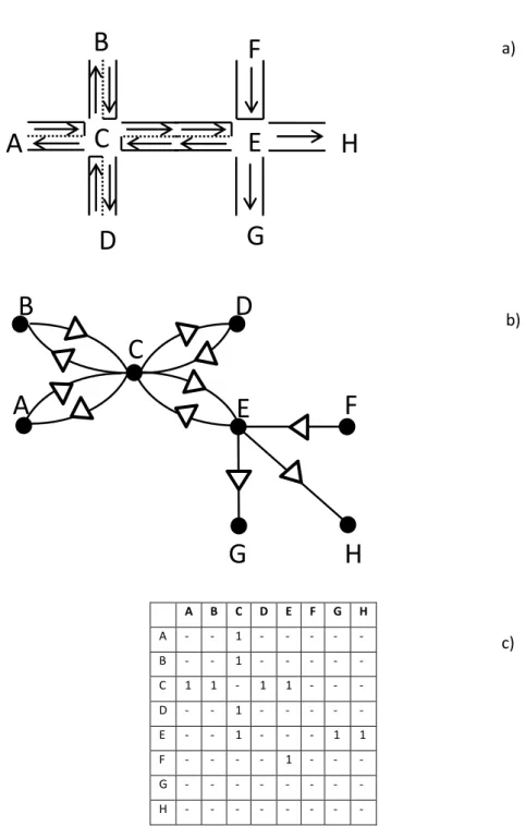
5.1 – Adjacency structure of the sensor network 114

5.2 – Graphical representation of the ITN 117

5.3 – Distances measured between sensor locations using Euclidean distance, LCAP (sensor) network distance and road network distance

119 5.4 – Illustration of the process of connecting the sensor (LCAP) network to the

physical (ITN) network

121 5.5 – Temporal autocorrelation in UTT for the 342 test links at the 5 minute

aggregation level

124

5.6 – Seasonal autocorrelation in LCAP data 125

5.7 – Illustration of the danger of spurious correlation 126

5.8 – ACF after first order differencing a) 180 lags shown. b) First 10 lags shown. 129 5.9 – Relationship between distance and CC at temporal lag zero 130 5.10 – Average cross-correlation between each link and its first 5 nearest spatial

neighbours

(9)

9

5.11 – Histogram of CCF values at temporal lag zero and spatial lags 1 and 2 combined

133 5.12 – 3D scatter plot of the relationship between correlation (z-axis), distance

(x-axis) and temporal lag (y-(x-axis)

134

6.1 – Diagram of the training data construction 150

6.2 – Illustration of temporal window 152

6.3 –Location of the test links on the LCAP network 157

6.4 – Time series of each of the test links over the first 10 weeks of the training period

158

6.5 – Fitted values of sigma with a window size of 1 167

6.6 – Fitted values of Lambda 0 with w=1 169

6.7 – Effect of varying σ through its range with Lambda fixed 170

6.8 – Effect of varying through its range with σ fixed 172

6.9 – Observed versus forecast values for link 442 176

6.12 – RMSE of each of the models 182

6.13 – MAPE of each of the models 184

7.1 – Network of core LCAP links within the CCZ 193

7.2 – Location of link 417 and its spatial neighbours 201

7.3 – Google street view snapshot of the intersection of links 417 and 447/455 202

7.4 –Real versus fitted values for link 417 204

7.5 –Real versus forecast values for link 417 205

7.6 – Real versus fitted values for link 1745 207

7.7 –Real versus forecast values for link 1745 208

7.8 – Links connected to the start camera of LCAP link 1745 209

7.9 – Selected neighbours for link 1745 210

7.10 – Selected neighbours for link 1747 214

7.11 – Real versus fitted values for link 1747 216

(10)

10

List of Tables

2.1 – Types of Network 21

2.2 – Basic terminology of graph 22

3.1 – Description of traffic variables 45

3.2 – Delays caused by traffic signals 48

3.3 - A comparison of forecasting models in the literature 60 4.1 – Deciles of mean number of observations per link with minimum and

maximum values

101 4.2 - Description of patch types used to replace missing data 105 4.3 – Percentage of each patch type after removal of inactive links 105 6.1 – The test links and their patch rates and frequency 155

6.2 – Training errors 164

6.3 – Fitted model parameters at each of the forecast horizons 165

6.4 – Testing Errors of the LOKRR model 173

6.5 – Comparison with benchmark models– average errors 180

7.1 – Summary statistics of the test network 193

7.2 – Summary of training performance 196

7.3 – Summary of testing performance 196

7.4 – Fitted values of neighbourhood size k for each scenario. 197

7.5 – Fitted values of w for each scenario. 198

7.6 – Fitted values of σ for each scenario. 198

7.7 – Training errors for the k-NN model in each of the scenarios 198 7.8 – Training errors for the k-NN model in each of the scenarios 199

7.9 – Details of the neighbours of Link 417 200

7.10 – Training results, link 417 201

7.11 – Testing results, link 417 201

7.12 - Training results, link 1745 205

7.13 – Testing results, link 1745 205

7.14 – Details of neighbours of Link 1745 210

7.15 –Training results, link 1747 211

7.16 –Testing results, link 1747 211

7.17 - Details of neighbours of Link 1745 212

(11)

11

Chapter 1 Introduction

1.1 Progress in network science

Networks are everywhere and human beings interact with them on a daily basis; commuting between home and work on transportation networks, accessing information on the World Wide Web over the Internet, communicating with others over mobile phone networks; all the while using the neural network in their brain to accomplish these tasks. Networks provide a rich metaphor for many real world processes, systems and structures, both physical and abstract.

Complex networks are those networks whose structure is irregular, complex and dynamically evolving in time (Boccaletti et al., 2006). Since the latter period of the 20th century, there has been an explosion of research into the structure and function of complex networks. This has evolved into the field of network science, which has produced significant scientific breakthroughs in terms of network structure, notably, many networks exhibit small world (Watts and Strogatz, 1998) and scale free (Barabási and Albert, 1999) properties. For example, in the study of road networks, a great deal of recent research has focused on topology, notably the influence configuration and connectivity hold on network usage and dynamics (Hillier and Iida, 2005; Castells, 2010; Pflieger and Rozenblat, 2010). Small world phenomena are also observed on transportation networks due to the interplay between network structure and the dynamics taking place on them (Xu and Sui, 2007). Jiang (2007) observes that the topologies of urban street networks based on street-street intersection exhibit scale free properties and follow a power law distribution, with 80% of streets having length or degree less than average and 20% having length or degree greater than average. This property has been shown to apply to traffic flow on street networks (Jiang, 2009).

Yet such research, although valuable in understanding the structure and properties of networks, fails to fully explain the nature of the spatio-temporal dynamics occurring on the network. Network processes are often characterised by spatio-temporal patterns of nonstationarity, nonlinearity and heterogeneity. The nonstationarity usually refers to the trends and seasonal/cyclic patterns, such as morning-peak and seasonal change of traffic flow on road network. The nonlinearity of spatio-temporal patterns could be in various forms, particularly heteroskedasticity, which is nonconstant variance in time and/or space (Stathopoulos and Karlaftis, 2001; Cheng et al., 2011; Cheng et al, 2013). Nonlinearity in

(12)

12

space is commonly referred to as heterogeneity, which is a term that encompasses the notion that the earth’s surface displays incredible variety (De Smith et al., 2007).

All these issues make the forecasting of network performance extremely challenging. Recently, models have been developed, for example, to simulate the spread of, and immunization against disease (Pastor-Satorras and Vespignani, 2002; 2005; Cohen et al., 2003), in both human populations and technological networks. But more efforts are needed on this front for many real world networks such as transport, electrical grids (U.S. Dept. of Energy, 2009) and the Internet. More importantly, with real time data collected on many real world networks, it is the time to move from structural analysis and simulation to the modelling and forecasting of these data.

1.2 Forecasting of network data

Forecasting models of network data have traditionally focussed on time series approaches. In such approaches, the network structure is ignored and each of the time series at the nodes is forecast independently. Examples of such models exist in electrical load forecasting (Alfares and Nazeeruddin, 2002; Hahn et al., 2009), Internet traffic forecasting (Basu et al., 1996; Papagiannaki et al., 2003) and road traffic forecasting (Vlahogianni et al., 2004), amongst others. While time series approaches can achieve excellent results, they ignore the spatio-temporal evolution of the network process, and often perform poorly under abnormal conditions and when data are missing (Vlahogianni, 2007).

More recent approaches use network structures to construct spatio-temporal models that capture the spatio-temporal dependency between locations where network data are observed. The traditional way to incorporate spatial structure into a forecasting model is to assume that the spatio-temporal relationship can be described by a linear model with global set of parameters, which requires the space-time process to be weakly stationary (Cressie and Wikle, 2011). However, such models typically cannot deal with the nonstationary and nonlinear properties of network data, especially when network data are highly dynamic (Kamarianakis and Prastacos, 2005; Cheng et al. 2013).

In response to this, statistical modelling frameworks have been extended to model local and/or dynamic space-time structures recently (Min et al., 2009a; Ding et al., 2010; Min and Wynter, 2011; Kamarianakis et al., 2012; Cheng et al, 2013). The improvement that these models gain over global model specifications is striking, and clearly motivates the use of

(13)

13

local model structures (Cheng et al, 2013). However, although these approaches are well grounded in statistical theory and show promising performance, the configuration of the spatial and temporal structure for such models is non-trivial, which makes their computation costly, and limits their application to large networks.

Increasingly, researchers and practitioners are turning towards less conventional techniques, often with their roots in the machine learning (ML) and data mining communities, that are better equipped to deal with the heterogeneous, nonlinear and mutli-scale properties of large scale network datasets. For instance, many of the ML methods that have recently proliferated in the time series forecasting literature have shown strong performance (Ahmed et al., 2010), particularly in the context of longer range forecasts (Vlahogianni et al., 2004). It has been demonstrated, for example, that a globally trained spatio-temporal artificial neural network (ANN) model can outperform a linear state-space model with a local space-time structure (Vlahogianni et al., 2007). Of these methods, kernel methods are particularly attractive as they combine the advantages of globally optimal linear models with nonlinear capabilities. However, these approaches mainly use globally fixed structures. How to combine the local spatio-temporal structure in ML models in order to improve their forecasting accuracy and explanatory power is a challenge for space-time forecasting of network data.

1.3 Challenges in modelling urban road networks

This thesis focusses on a particular type of spatial network (Barthélemy, 2011), the urban road network. The smooth operation of urban road networks is fundamental to the health of cities worldwide. Poorly functioning road networks have severe economic, social and environmental costs related to traffic congestion, environmental pollution and public safety (Arnott and Small, 1994; Walters, 1961; Goodwin, 2004; Barth and Boriboonsomsin, 2008). Because of their importance, many urban road networks are equipped with sensor networks that observe the traffic stream for a variety of purposes such as enforcement, incident detection and traffic monitoring (Chong and Kumar, 2003). On a sensor network, a time series of observations of the network process is collected at each node of the network. These data are used in forecasting systems to aid urban traffic control systems (UTCS), advanced traffic management systems (ATMS) and advance traveller information systems (ATIS) (Vlahogianni et al., 2004).

(14)

14

To make best use of this data, it is necessary to take a network-based approach, which enables modelling of the spatio-temporal evolution of traffic conditions. If one can model the way in which the current process evolves from its past values, then one can model causation, which is the “holy grail of science” (Cressie and Wikle, 2011, p.297). In other words, one can model the spread of congestion. This is particularly important in the context of non-recurrent events, whose spatio-temporal effect can be large. Despite this, the uptake of spatio-temporal models in the traffic forecasting literature has been slow, and there are very few models that have been developed for large scale forecasting of urban road networks (Yue and Yeh, 2008). Historically, the main reason for the slow uptake and development of spatio-temporal models has been the lack of available data and computational power (Griffith, 2010). This situation has now been reversed, and replaced with the problems of modelling so called big data (Lynch, 2008; Boyd and Crawford, 2011; Manyika et al., 2011). In the context of traffic data, these problems can be summarised around three points:

Firstly, large scale network data are often subject to high levels of noise and missing data that must be dealt with on the fly (Zhong et al., 2004a; Griffith, 2010; L. Li et al., 2013). Missing data periods are often lengthy and not randomly dispersed in the data (Qu et al., 2009). Missing data are usually ignored in the context of forecasting, and dealt with offline using imputation (Zhong et al., 2004a). This is insufficient to maintain forecasting performance in real time. A small number of recent studies have attempted to address this by accounting for missing data in the forecasting algorithm (Whitlock and Queen, 2000; van Lint et al., 2005; Chan et al., 2013b), but they are applied to highway data where the spatio-temporal dependency relationships are more certain. Application to urban networks has not been considered, despite being a serious problem.

Secondly, due to the prohibitive cost of installing and maintaining sensor networks, as well as processing and storing data collected using them, sensors are often sparsely located in space (Liu, 2008), and do not have sufficient spatial coverage to model the physical relationship between locations in an unambiguous manner. The idealised representation of the network structure that one would expect is often not mimicked in the sensor network structure, and must be elicited (Haworth et al., 2013). Furthermore, one typically has to develop models from sensor networks that were not constructed with forecasting in mind. Often the spatio-temporal relationships between locations are nonlinear, heterogeneous and weak, and difficult to model using conventional methods (Cheng et al., 2011).

(15)

15

Finally, the sheer amount of data being collected means that network models must be capable of processing incoming data and producing forecasts in a timely fashion. This leads to a trade-off between the complexity of the process that can be modelled and the computational efficiency of the algorithm. This is a difficult task, and consequently the spatio-temporal models of urban networks described in the literature are typically applied to small networks, which are not indicative of the networks of entire cities. Linked to this problem is the issue that network processes are dynamic, and models must be able to adapt to changes in the data distribution over time in order for performance to be maintained. Such models are known as online, and have only been developed in a small number of studies to date in the context of freeway data (Castro-Neto et al., 2009; van Lint, 2008). Application of online algorithms to urban road networks has not been attempted.

1.4 Research objectives

In light of the challenges described in the preceding sections, the aim of this thesis is to develop a forecasting model of network data that fulfils the following research objectives: Objective 1 – To develop a framework for modelling the spatio-temporal structure of real world network data.

Objective 2 – To integrate the spatio-temporal structure of networks into a forecasting model that is capable of operating in real time, and is robust to the presence of missing data. Objective 3 – To apply the model to the case of forecasting travel times on an urban road network, where the sensor network is sparsely deployed on a dense road network. Objective 4 - To develop an evaluation framework for assessing the strengths and weaknesses of the proposed model.

1.5 Scope of the thesis

There are many potential sources of traffic data on London’s road network. Many of the signalised intersections are controlled by Split Cycle Offset Optimisation Technique (SCOOT), and this system collects flow, delay, congestion, detector occupancy and detector flow (Imtech, 2013). Transport for London also maintains an incident database called the London Transport Information System (LTIS), which has details of planned and unplanned road works, incidents etc. Aside from this, floating vehicle data obtained from mobile phone and

(16)

16

GPS devices are becoming more widespread. In each of these data sources there are non-trivial issues with data processing and/or acquisition that complicate their use.

This thesis concentrates on the short term forecasting of travel time data collected using automatic number plate recognition (ANPR) data as part of Transport for London’s (TfL) London Congestion Analysis Project (LCAP). In this context, short term forecasting is taken to mean forecasting of intra-day traffic. The application to long term forecasting of traffic variables for planning purposes is not considered, although it is an important problem in its own right.

In accordance with the scope, the literature review section of this thesis is focussed primarily on methods for forecasting road network data. However, the proposed model is not tailored to the specific problem of forecasting road network data. Extensions to the model framework are given in the concluding chapter that suggest ways of applying the model in a wider context.

1.6 Structure of the thesis

This thesis is organised into nine main chapters and two appendices that contain supplementary material and additional results that are not presented in the main body of the thesis. A roadmap of the thesis structure is shown in figure 1.1. The content of the chapters is as follows:

In Chapter 2, entitled Networks, the basic concepts and terminology of networks are introduced. Particular attention is paid to spatial networks in order to limit the scope of the review. Methods for forecasting network data are introduced.

Chapter 3, entitled Spatio-temporal forecasting of road network traffic reviewsthe progress to date on modelling and forecasting of traffic data collected on road networks. The chapter focusses on three facets of the models described in the literature: 1) the types of model that have been used, which are broadly separated into parametric and machine learning approaches; 2) the ways in which spatio-temporal information are incorporated into the models, with particular attention paid to those models that are applied to urban road networks, and; 3) the ways in which missing data are dealt with in forecasting models. The findings of this chapter motivate the direction of research in chapters 4, 5 and 6.

(17)

17 Figure 1.1 – Thesis roadmap

In Chapter 4, entitled The London Congestion Analysis Project, the case study data is introduced, which is the London Congestion Analysis Project (LCAP). The LCAP is a network of automatic number plate recognition (ANPR) cameras that collect travel time data on London’s road network. A thorough missing data analysis is presented.

Chapter 5, entitled Modelling the LCAP Network, describes how the LCAP network can be modelled using a spatial weight matrix. The sensor network is fused with the physical road network in order to produce a better representation of the spatio-temporal relationship between sensor locations. A space-time autocorrelation analysis is carried out that reveals a pattern of strong temporal autocorrelation and weak spatio-temporal autocorrelation. Based on these findings, and the findings of Chapters 3 and 4, some requirements of a space-time model of network data are defined.

(18)

18

In Chapter 6, entitled Local Online Kernel Ridge Regression, a temporally local forecasting model is described for forecasting of seasonal time series data. The model is kernel based, in which small kernels are defined for each time of day, each with their own parameters. The model is online and is able to accommodate new data as they arrive. Although applied to traffic data, the model is applicable to any time series that displays cyclic variation, and can be extended to other types of time series.

In Chapter 7, entitled Spatio-temporal LOKRR for forecasting under missing data the LOKRR model is extended to incorporate the spatial structure of networks. The spatio-temporal (ST)LOKRR model is applied to forecasting of travel times where data are assumed to be missing due to sensor failure.

In Chapter 8, entitled Model Evaluation and Extensions, the model evaluation framework is described, against which the performance of the LOKRR and STLOKRR models is evaluated. Based on the results of the evaluation, some model extensions are briefly described that will form part of the basis for future research.

Finally, in Chapter 9, entitled Conclusion, the thesis is concluded. The main outcomes of the research are stated, and the contributions to the scientific literature are elucidated. The thesis ends with a statement about the future directions for research in the subject area.

(19)

19

Chapter 2 Networks

2.1 Chapter overview

This chapter charts the progress to date in modelling networks, with particular attention paid to spatial networks. In section 2.2, networks are defined, and a brief introduction to complex networks and the field of network science is given. The aim of this section is not to provide an exhaustive survey of the network science literature, but to alert the reader to some of the major achievements of network science. Section 2.3 contains a discussion of network processes, and how they can be incorporated into mathematical models. Section 2.4 introduces spatial network structures, and how they differ from other networks, before the properties of spatio-temporal processes are introduced in section 2.5. In section 2.6, parametric and machine learning (ML) approaches to modelling spatio-temporal network data are described, and the main approaches are reviewed. Finally, the Chapter is summarised in section 2.7.

2.2 Background: Networks, complex networks and network science

A network is a set of discrete items, called nodes, with connections between them, called

edges. A network is typically represented as a graph G = (N, E), with a set of N nodes and E

edges. Networks can be broadly separated into four categories, which are social networks, information networks, biological networks and technological networks (Newman, 2003). Table 2.1 summarises these types of network and some basic terminology of graphs is given in table 2.2. These terms are used throughout this thesis.

Since the 1990s, much research on networks has focused on the theory of complex networks, which are those networks whose properties are irregular, complex and dynamically evolving in time (Boccaletti et al., 2006). The study of such networks has been facilitated by increases in computing power and the availability of massive datasets pertaining to real life networks, as well as the emergence and growth of new types of networks in the digital world such as the Internet and online social networks.

Ground-breaking research has revealed that certain structural properties pervade many types of network, notably the small world property (Watts and Strogatz, 1998) and the scale-free property (Barabási and Albert, 1999). A scale scale-free network is one whose degree

(20)

20

distribution follows a power law. Many real world networks have been shown to be scale free, including the World Wide Web and social networks.

Table 2.1 – Types of Network (Summarised from Newman, 2003)

Type of network Description Examples

Social Network A set of people (or animals) or groups of people (nodes) with associations between them (edges).

Friendship networks Academic collaborations Business relationships Animal behaviour Information Network

Networks of information flow. Pieces of information are stored at the nodes. The edges between nodes signify connections between information sources.

Academic citation networks. World Wide Web

Biological Network

Networks of biological systems, where the nodes are biological entities, and the edges are connections between them. Metabolic Networks Neural Networks Food Webs Technological Network

Man-made, physical networks, designed to transport people, resources or commodities.

Transportation networks (Roads, rail, airlines)

The Internet Electricity Grid

In a scale free network, a small number of nodes are highly connected and have huge importance within the network. In a small world network, the typical distance between two nodes grows proportionally with the logarithm of the number of nodes in the network, which essentially means that a path between any two nodes in the network will typically consist of a small number of steps. Small world networks are themselves scale free. The discovery of these properties has been tremendously important in shaping our understanding of networks, and has led to important research into the resilience of networks (Dobson et al., 2007), the growth of networks (Albert and Barabási, 2002) amongst other things.

(21)

21

The surge in research has led to various works being published that summarise the progress to date in the study of complex networks and attempt to formalise the concepts in terms of graph theory (see, for example, Albert and Barabási, 2002; Newman, 2003; Boccaletti et al., 2006). The early work formed the building blocks of the field of network science, which has now become a mature subject in its own right, exemplified by the creation in 2013 of the

Network Science journal by Cambridge University Press (Brandes et al., 2013). The network science literature provides a diverse range of tools and techniques for analysing and enhancing our understanding of the structure and large scale statistical properties of networks.

Table 2.2 – Basic terminology of graphs

Term Definition

Directed Edge An edge with an associated direction. It is directed from its

start node to its end node

Directed graph (digraph) A graph in which all the edges are directed Undirected graph A graph that contains no directed edges

Adjacency Two nodes in a graph are considered to be adjacent if they are connected by an edge. Likewise, two edges in a graph are considered to be adjacent if they share a common node. Incidence If node n is an node of an edge e, then n is incident on e, and

vice versa.

Node degree The degree of a node n in graph G, denoted deg(n), is the number of edges incident on n plus twice the number of self-loops. Self-loops are not considered in this thesis.

Weighted graph A graph in which each edge is assigned a number, called an edge weight.

Path A sequence of edges that connects a sequence of nodes in a graph.

2.3 Modelling Network Processes

The processes that take place on networks can be of equal interest to the structure of networks themselves. For example, in social networks, the nodes and edges themselves are of great interest because they reveal the structural properties of social relationships.

(22)

22

However, it is difficult to understand why such properties exist without examining the

attributes of the nodes. Looking at the attributes allows one to answer questions such as:

what characteristics make a certain node more connected than another node? And; what characteristics do connected nodes share? In complex networks, it is a reasonable assumption that nodes that are connected by an edge will be similar in some way. More specifically, one or more of their attributes will be correlated.

It is the interplay between the processes occurring on networks and the complexity and dynamics of the network structure where there is great potential for research. The ultimate goal of the study of the structure of complex networks is to gain an understanding of the systems built upon them (Newman, 2003). For example, one may wish to explore how the structure of a social network affects the spread of information in times of crisis or political unrest such as the Arab Spring that began in 2010 (Lotan et al., 2011; Khondker, 2011) or the London riots of 2011 (Tonkin et al., 2012); or one may wish to know how network structure causes congestion and cascading failures in flow networks (Albert et al., 2000; De Martino et al., 2009; Holme, 2003; Rosas-Casals et al., 2007; Zhang and Yang, 2008).

2.3.1 Adjacency matrices

To analyse and model a network process, a network can be represented mathematically using an adjacency matrix. Given an undirected graph with nodes and edges, an adjacency matrix is an square matrix. Its element is 1 if nodes and are adjacent. That is, . For an undirected network, the adjacency matrix

is symmetric, and its leading diagonal is zero provided it does not contain any loops (edges with the same start and end node)1. Adjacency matrices are convenient as they can be used directly in correlation measures and regression models. For instance, a network autoregressive model can be written as:

(2.1)

1

Alternatively, one may define an incidence matrix, which is an matrix. In its simplest form, it is a binary matrix where the element is 1 if node is incident on edge , 0 otherwise.

(23)

23

Where is the network lag coefficient, is the vector of dependent variable values and is the vector of error terms (Peeters and Thomas, 2009). Here, the adjacency matrix is usually row standardized so that all rows sum to one, which has the effect of including a weighted sum of the values at adjacent nodes in the regression equation (De Smith et al., 2007). In a network autoregressive model, the dependent variable appears on both sides of the equation because is modelled as a linear combination of lagged values of itself, recorded at adjacent nodes in the network.

This type of model is common in the field of network autocorrelation analysis, which emerged independently of the complex networks literature in the late 1970s. Network autocorrelation borrows techniques from spatial analysis and geography as tools for analysing data collected on networks. Network autocorrelation models aim to model the relationship between variables measured at the nodes of a network. They were first applied to social and cultural data. Dow et al. (1982) extend the spatial autocorrelated disturbances (errors) model to the network case by changing the structure of the spatial weight matrix to reflect network linkages. In this type of model, the errors are not independent and are considered as a weighted average of the errors at related units, determined by the weight matrix (Dow et al., 1984).

Various extensions to this method have been devised and the effect of different network structures on spatial and network autoregressive models is examined in Farber et al. (2009). A diverse range of tangible and intangible networks have been modelled including social networks (Doreian et al., 1984; Dow et al., 1984; Dow, 2007; Dow and Eff, 2008; Leenders, 2002), migration networks (Black, 1992; Chun, 2008) and transportation networks (Black and Thomas, 1998; Flahaut et al., 2003).

2.4 Spatial Network Structures

A spatial network is a particular type of network whose nodes are embedded in Euclidean space, and whose edges are real physical connections (Boccaletti et al., 2006). Spatial networks have unique characteristics that require different treatment to aspatial networks. The principal influence on the structure and function of spatial networks is the physical distance between nodes. On spatial networks, the presence of an edge between two nodes is limited by their physical separation distance. For example, in the network of airports, a route (edge) can only exist between two airports (nodes) if their separation distance does not exceed the maximum range of aircraft.

(24)

24

Spatial networks can be planar. A planar network is one whose edges do not intersect when drawn in the plane (Barthélemy, 2011). In planar spatial networks, such as road networks and river systems, the degree of a node is constrained by the physical space available for edges (Boccaletti et al., 2006). For instance, in the planar representation of a road network, the number of road segments that join at an intersection is constrained by the space available for roads. It is uncommon to encounter intersections that connect more than 5 or 6 road sections. Hence, planar networks necessarily cannot be scale free (Cardillo et al., 2006)2. The airport network is a spatial network that is not planar as routes may cross one another.

2.4.1 Spatial weight matrices

The network metaphor has been used to represent geographical space in quantitative geography for over 40 years (Barthélemy, 2011). The quantitative modelling of spatial processes using a network representation is achieved using spatial weight matrices. Given a network of spatial units , with spatial units and edges connecting them, a spatial weight matrix W is an square matrix in which the element .

The difference between W and an adjacency matrix is that its elements need not be binary, meaning that it can contain a much richer representation of the geographic space. Cliff and Ord's (1969) seminal work demonstrates that a weight matrix representing various types of spatial connections can better account for the nuances of real world spatial dependencies than a binary matrix (Getis, 2009).

A non-binary weighting scheme in W equates to representing the spatial units as a weighted graph. The choice of the weights is application specific and allows one to incorporate prior knowledge of the spatial process into a model. For example, in the case of areal data the weights may be specified as the length of the shared border, the proportion of shared perimeter or the number of neighbours (Getis and Aldstadt, 2004). If W is symmetric, the relationship between locations is assumed to be identical in both directions, meaning that the perceived influence of unit on unit is equal to the perceived influence of unit on unit . If W is asymmetric then direction is introduced to the system, which equates to being a directed graph. Directed graphs are used in systems of flows, such as transportation networks.

2_{Road networks need not be represented as planar and can be based, for example, on street-street}

(25)

25

Determining the weighting structure and the value of the weights in W is a non-trivial issue. Different weight matrices can lead to different inferences being drawn and can induce bias in models. The effect of this has been explored in the spatial literature (see Stetzer, 1982; Florax and Rey, 1995; Griffith and Lagona, 1998) and the networks literature (Mizruchi and Neuman, 2008; Páez et al., 2008; Farber et al., 2009; Neuman and Mizruchi, 2010). On spatial networks, network distance between neighbouring units can be used as the weighting scheme, although this is not always straightforward. Direction of dependence is often important, and may change with time, and the dependence may not decay linearly with spatial distance.

2.5 Spatial Network Processes

There are many different types of process that operate on spatial networks. This thesis is concerned primarily with flow networks, in which some quantity flows between the nodes of the network along the edges. Examples of flow networks are transportation systems, the Internet and electrical grids. On flow networks, observations of the network process are (usually) made at regular intervals using sensors, which form time series. These sensors are distributed across the network, and when considered together form a space time series that describes the network process. The processes that are observed on spatial networks typically exhibit characteristics that require special treatment in space-time modelling frameworks. In the following sections, the temporal and spatial characteristics of spatial networks are described in turn.

2.5.1 Time series

Observations of a space-time process are made at the nodes of a spatial network, which are sampling locations such as weather stations, traffic flow detectors or census output areas. At each node an individual time series is collected that describes the temporal evolution of the space-time process at a single point in space. A time series { } in temporal domain is a sequence of observations of a process, usually taken at equally spaced time intervals; , where denotes the value of some quantity such as

traffic flow volume at time and is the length of the series. indicates the time at

(26)

26

2.5.1.1 Stationary process

A strictly stationary process is one whose joint probability distribution does not change with time, which entails that the joint probability distribution of a series with observations

made at any set of times is the same as

that associated with observations recorded at another set of times , for any choice of , which is known as the temporal lag (Box et al., 1994, p.24). A strictly stationary process has constant mean and variance. The joint probability distribution is also the same for all values of , meaning that the

autocovariance between and is equal for all .

2.5.1.2 Temporal dependence and autocorrelation

An observation from nature is that near things tend to be more similar than distant things in time. For instance, the weather tomorrow is more likely to be similar to today’s weather than the weather a week ago, or a month ago and so on. This phenomenon is known as temporal dependence. The presence of temporal dependence violates the stationarity property described in section 2.5.1.1 that is a requirement of classic statistical models such as ordinary least squares (OLS). Temporal dependence can be measured using the temporal (or serial) autocorrelation function3 (ACF, see, for example, Box et al., 1994). Autocorrelation is the cross-correlation of a series with itself. It is calculated at discrete temporal lags and, for interpretability, is usually displayed as an ACF plot with confidence intervals shown (see figure 2.1).

If a time series exhibits autocorrelation that does not decay exponentially toward, and remain at, zero then it is nonstationary, meaning it does not have constant mean and variance. If the autocorrelation decays toward zero initially but returns to significant positive values at regularly spaced intervals, then the series contains a seasonal (cyclical) pattern. This type of pattern is common in many series, including traffic data where it is caused by rush hour traffic patterns. Many linear time series models, such as the autoregressive integrated moving average (ARIMA) model, require removal of autocorrelation from the series prior to model building in order to be effective. This is usually accomplished through seasonal or nonseasonal differencing (Kendall and Ord, 1990, p.37-39).

3

(27)

27

Figure 2.1 – A typical ACF plot showing strong, significant autocorrelation, decaying exponentially toward zero. Approximate 95% confidence intervals are shown as blue,

horizontal lines. Note that the autocorrelation at lag zero is always 1.

2.5.1.3 Nonlinearity

Some time series exhibit nonlinear characteristics. The term nonlinear is somewhat ambiguous; for instance, if a series can be explained by a simple analytic function such as a power, sinusoid or exponential then, although nonlinear, it can often be linearized and modelled with linear techniques (Cook, 1987). Hence, series of this type are usually not considered to be nonlinear in the time series literature. Here, nonlinear is taken to mean those time series that cannot be modelled using linear techniques. An example of a nonlinear series is a cyclic time series that increases at a faster rate than it decreases, or vice versa (Chatfield, 2004). In such series, future values of the series do not depend linearly on previous values. Nonlinear series of this type cannot be explained by a linear model and may benefit from a nonlinear approach. There are various methods for testing for nonlinearity in time series which are reviewed in Tsay (1986). Lee et al. (1993) compare a range of the available methods. In the presence of nonlinearity, a range of nonlinear time series techniques have been developed including bilinear models (Granger, 1978) and machine learning techniques such as Artificial Neural Networks (ANNs) ANNs and Support Vector Regression (SVR).

(28)

28

2.5.1.4 Heteroskedasticity

One very common form of nonlinearity that is common in real time series is heteroskedasticity. Heteroskedasticity is present in a time series when its variance is not constant over time. This has been recognised as a particular problem in financial series where volatility clustering is common (Mandelbrot, 1963). It is also present in flow networks, where variance is higher in peak periods. Like temporal dependence, this property violates the assumption of stationarity; and leads to consistent but inefficient parameter estimates and inconsistent covariance matrix estimates (White, 1980). The autoregressive conditional heteroskedasticity (ARCH) model of (Engle, 1982) was developed specifically to deal with this phenomenon. As with an ARIMA model, it is applied to uncorrelated, zero mean time series but the conditional variance is modelled as nonconstant. Engle won the Nobel Prize in 2003 for his contribution, and the basic method has since been widely applied, modified and extended and Engle (2001) provides a summary. Traffic series are heteroskedastic as the variance is higher during congested periods (Fosgerau and Fukuda, 2012).

2.5.2 Spatial characteristics

When a variable is observed at two or more locations it can be considered a spatial series { } in spatial domain . At each time , the series of observations collected at the nodes of a spatial network forms a spatial series. Spatial series share many of the characteristics of time series, but they are fundamentally different because space is two or three dimensional whereas time is one dimensional and unidirectional.

2.5.3 Spatial stationarity

A stationary spatial process is one whose mean and variance are constant in space. The covariance between observations of the processes depends only on their separation distance (Cressie, 1988). Firstly:

[ ]

(2.2) Secondly:

[ ]

(29)

29

If is a function only of the distance between and then the process is also isotropic, which means that the variance is constant in all directions.

2.5.4 Spatial dependence and autocorrelation

Like temporal data, spatial data often violate the normality assumptions required by standard statistical models because they exhibit spatial dependence. This phenomenon is neatly summed up neatly by Tobler’s famous first law of geography:

“Everything is related to everything else, but near things are more related than distant things” (Tobler, 1970).

To give an example, if one were supplied with some precise GPS coordinates in middle of the Sahara desert, one may infer with some degree of certainty that the terrain type would be desert. To make this inference, one would only require knowledge of the Sahara and nowhere else. Although this is a simple example, the general concept underlies the whole field of spatial analysis. Temporal dependence may be present in any type of network data, but spatial dependence is unique to spatial network data. It limits dependencies between nodes in the network that are spatially distant, thus allowing for sparse model structures. Spatial dependence can be measured using an autocorrelation function that makes use of a spatial weight matrix. The two best known measures of spatial autocorrelation are Moran’s I (Moran, 1950) and Geary’s C (Geary, 1954) which are both global indices. Of these, Moran’s I has been adopted most widely in the literature.

2.5.5 Spatial Heterogeneity

Spatial data often exhibit structural instability over space, which is referred to as heterogeneity. Heterogeneity has two distinct aspects; structural instability as expressed by changing functional forms or varying parameters, and heteroskedasticity that leads to error terms with non-constant variance (Anselin, 1988). Ignoring it can have serious consequences including biased parameter estimates, misleading significance levels and poor predictive power. Anselin (1988) provides some methods for testing for heterogeneity. Additionally, a number of local indicators of spatial association (LISA), a term coined by Anselin (1995), have been devised. These include a local variant of Moran’s I (Anselin, 1995) and Getis and Ord’s and statistics (Getis and Ord, 1992), which measure the extent to which high and low

(30)

30

values are clustered together. A description of these and other spatial autocorrelation indicators can be found in (De Smith et al., 2007).

2.5.6 Interaction of spatial and temporal characteristics on networks

Dealing with spatio-temporal data involves dealing with the dynamics of spatial and network processes. The spatial and temporal dimensions in isolation provide a narrow view of the behaviour of a network process, but when combined they can describe the evolution of the process over time. If the spatio-temporal dependence in a network can be modelled then one essentially has predictive information. However, modelling space-time data is rarely simple as it combines the problems of dealing with spatial and temporal processes separately. The behaviour of a variable over space differs from its behaviour in time. Time has a clear ordering of past, present and future while space does not and because of this ordering isotropy has no meaning in the space-time context (Harvill, 2010). In time, measurements can only be taken on one side of the axis; hence estimation involves extrapolation rather than interpolation (Kyriakidis and Journel, 1999). Temporal data also has other characteristics, such as periodicity, that are not common in spatial data and scales of measurement also differ between space and time and are not directly comparable. Adequately accounting for these differences is essential in a model characterizing spatio-temporal behaviour (Heuvelink and Griffith, 2010).

2.6 Models of spatio-temporal network data

In this section, the main approaches to space-time modelling of spatial network data are introduced. The review covers methods that are capable of being applied to network structures. As such, many of the methods are not applied to data that would be conventionally viewed as network data, but to other types of spatial data that can be represented in a network structure. According to the scope of this thesis, the review is intentionally brief. A more detailed review of the literature on space time modelling of traffic data is given in Chapter 3. Broadly, there are two approaches that can be taken to model a space-time network process. The first approach is to explicitly model the spatio-temporal relationship between locations in a parametric framework. The second approach is to learn the dependencies form the data using a machine learning (ML) approach. These two approaches are summarised in section 2.6.1. Following this, in sections 2.6.2 and 2.6.3, the

(31)

31

parametric and ML models that can be applied to spatio-temporal and network data are reviewed, respectively.

2.6.1 Parametric versus machine learning methods: An overview

The literature on space-time forecasting can be broadly separated into two categories of model that come from two different modelling paradigms. The first type is the statistical parametric model. A parametric model is one where the functional form of the relationship between the dependent and independent variables is described by a set of parameters. Linear least squares regression is the archetypal parametric model. Because of their unique properties, specialised parametric techniques are typically used to model spatio-temporal data. They are usually based on some form of autoregression (AR), whereby the current value of a series is modelled as a function of its previous values. The space-time autoregressive integrated moving average (STARIMA) model is a general parametric modelling framework for spatio-temporal data (Pfeiffer and Deutsch, 1980). Such models are theoretically well founded and are able to deal explicitly with the fundamental properties of spatio-temporal data. They are incredibly powerful and inherently interpretable provided that the model assumptions hold. However, these assumptions, such as stationarity, are often difficult to fulfil (Cheng et al., 2011). As more and more real world datasets become available at higher spatial and temporal resolutions, the task of describing space-time structures with conventional methods becomes more difficult.

ML provides an alternative approach. ML models were borne out of the need to model complex, nonlinear, non-stationary relationships in massive, real world datasets, often where little is known about their functional form. They typically make minimal assumptions about the process that generates the data, and instead seek to find a function that generalises best to unseen data. A function with good generalisation ability can be seen to implicitly capture the underlying process generating the data, which is commonly referred to as learning. This implicit learning is a fundamental difference between statistical and machine learning methods and is shown graphically in figure 2.2.

(32)

32

Figure 2.2 – Comparison of nature, statistical models and machine learning: a) in nature, input variables x are related to response variables y by some natural process. b) Statistical

models assume a stochastic data model that must be estimated. c) Machine learning assumes processes are unknown and seeks a mapping function from x to y. (Example

reproduced from Breiman (2001).

The general learning task is usually to find a mapping function between a limited set of input/output pairs { }, referred to as training data, where is the number of training examples. This task is known as supervised learning4. If the data are continuous then this is a regression problem, however, the approach taken to solve such problems in machine learning is different to that of classical statistics. Usually, in regression one seeks to minimise the empirical risk/error, which essentially means seeking the function that maps the inputs to the outputs with the lowest error, based on a loss function such as the sum of squared errors (SSE). This is, for example, the goal of linear least squares regression. For empirical risk minimisation to be a sensible goal, the data must be independent and identically distributed (i.i.d.) so that all future examples follow the same distribution and can be described by the same function. In reality, the data available for training a model are often noisy, and empirical risk minimisation based on a small number of training samples can lead to overfitting and poor generalisation ability. The problem is exacerbated when one is searching within a space of nonlinear functions that machine learning algorithms allow. For example, given a sufficient number of neurons, an ANN will fit the input data exactly, resulting in zero training error but poor generalisation ability. Conversely, there is also the problem of underfitting that occurs when the chosen function is too simple, which also leads to poor generalisation ability.

4_{If there are no associated outputs then it becomes a problem of unsupervised learning. This is not}

(33)

33 Figure 2.3- The concept of overfitting and underfitting

Finding an appropriate model can be seen as a trade-off between model bias and variance. In this context, bias is the expected generalisation error of the model, while variance is the extent to which the variance in the training data is modelled. Figure 2.3 a) represents a model with low variance but high bias, whereas figure 2.3 c) has low bias but high variance. Both models would have poor generalisation ability. Figure 2.3 b) has a better trade-off between the two and would be expected to generalise better to unseen data. One of the major contributions of the machine learning literature is the development of techniques for learning functions that attempt to control the bias variance trade off. Cross-validation is a simple example of this, whereby one seeks to find a function of the training data that is best able to predict an independent testing or validation set. -fold cross-validation is often used whereby the training data is partitioned into subsets which are each predicted in turn using the remaining subsets. In this way, the generalisation erroris minimised rather than the empirical error. This type of approach has been adopted in the spatial sciences with k-fold cross validation being important in Geographically Weighted Regression (GWR) model selection (Fotheringham et al., 2002). Other types of cross-validation include leave one out, holdout and bootstrapping, which are compared by Kohavi (1995). Browne (2000) provides a detailed review.

A complementary approach to cross-validation is regularization, which involves penalising a model based on its complexity, or number of parameters. The Akaike Information Criterion (AIC, Akaike, 1974) is a method commonly used for parameter selection in statistical models that controls the tradeoff between bias and variance. ARIMA models are often fit based on the AIC. In ML, the structural risk minimisation principle is often used for model selection, which makes use of the Vapnik-Chervonenkis (VC) dimension (Vapnik and Chervonenkis, 1971) to determine probabilistic upper bounds on the training error over a set of hypothesis spaces. The hypothesis space with the tightest error bound can be chosen as the best model (Schölkopf et al., 1999). Structural risk minimisation is the key idea behind Support Vector

Spatio-temporal forecasting of network data