manuscript No.
(will be inserted by the editor)
A stable matrix version of the fast multipole method: stabilization
strategies and 1D examples
Difeng Cai · Jianlin Xia
Received: date / Accepted: date
Abstract The fast multipole method (FMM) is an efficient method for evaluating matrix-vector prod-ucts related to certain discretized kernel functions. The method involves an underlying FMM matrix given by a sequence of smaller matrices (called generators for convenience). Although there have been extensive work in designing and applying FMM techniques, the stability of the FMM and stable FMM matrix factorization have rarely been studied. In this work, we propose techniques that lead to stable operations with FMM matrices. One key objective is to give stabilization strategies that can be used to provide low-rank approximations and translation relations in the FMM satisfying some stability re-quirements. Standard Taylor expansions used in FMM methods yield basis generators susceptible to instability. Here, we introduce some scaling factors to control relevant norms of the generators and give rigorous analysis on the bounds of entrywise magnitudes. The second objective is to use the one-dimensional case as an example to show how to intuitively construct FMM matrices satisfying some stability conditions and enable stable matrix-vector multiplications. The third objective of the work is to bridge the gap between the FMM and stable FMM matrix factorizations. This is done by con-verting an FMM matrix into a hierarchically semiseparable (HSS) form that admits stable ULV-type factorizations. The HSS construction is done analytically with some tree strategies and does not need expensive algebraic compression used in other HSS methods. The fourth objective is to discuss the nu-merical stability and show that the resulting matrix forms are suitable for stable operations. Note that the essential stabilization ideas also apply to higher dimensions. Extensive numerical tests are given to illustrate the reliability and accuracy.
Keywords Numerical stability · Fast multipole method· FMM matrix · Scaling factor ·Low-rank approximation
Mathematics Subject Classification (2010) 65F30·65F35·15A23·15A60
1 Introduction
Let κ(x, y) be a kernel function in a form such as 1/(x−y), 1/(x−y)2, log(x−y) , and log|x−y|, where x, y∈C,x6=y. Given a set of points
s≡ {x1, . . . , xn}, xi∈C, (1)
letAbe ann×ndiscretized matrix with entries
Aij =κ(xi, xj), i6=j. (2)
The research of Jianlin Xia was supported in part by an NSF grant DMS-1819166. D. Cai
Department of Mathematics, Emory University, Atlanta, GA 30322, USA E-mail: [email protected]
J. Xia
Department of Mathematics, Purdue University, West Lafayette, IN 47907, USA E-mail: [email protected]
(The diagonal entriesAii are defined separately and do not concern us so far.) It is well known that the fast multipole method (FMM) [13, 25] can be used to evaluate the product ofAwith a vector to a given accuracy in linear complexity. As shown in [28], the FMM essentially yields a hierarchical structured approximation to A to a given accuracy. Such a structured approximation is also an example of an
H2-matrix [15, 17]. For convenience, we refer to this approximation derived with the FMM procedure as an FMM matrix.
The construction of an FMM matrix often involves appropriate degenerate approximations or trun-cated expansions of κ(x, y). Commonly used expansions are Taylor expansions, multipole expansions, and spherical harmonic expansions. Such expansions provide a convenient way to obtain low-rank ap-proximations of some off-diagonal blocks (κ(xi, yj)))xi∈x1,yj∈x2 ofAthat correspond to well-separated subsetsx1 andx2 ofs. (This will be made more precise later.)
In previous work on the FMM, the quality of the low-rank approximations resulting from expansions ofκ(x, y) is rarely studied in terms of the numerical stability. For example, Taylor expansions have been frequently used, but the resulting low-rank basis matrices may have terms that are very large, although the original matrix entries κ(xi, yj) may only have modest magnitudes. Examples of such terms are factorials and powers. The artificially large terms may lead to stability issues in matrix operations using the low-rank forms due to the magnification of numerical errors. This prevents the method from reaching high accuracies, as indicated in [14]. To ensure that the FMM matrix can be used for stable matrix computations, it is important to study the relevant numerical stability. A heuristic strategy to improve the stability is briefly mentioned in [14] without justification or guarantee of the performance. The numerical stability issue is also mentioned in [10] without any fix.
Thus, the first objective of this paper is to analytically obtain low-rank basis matrices and certain translation matrices used in the FMM that satisfy some stability requirements. More specifically, based on Taylor expansions ofκ(x, y), we design a scaling strategy where some appropriate scaling factors are chosen to modify the individual terms in the expansions. Then for well-separated subsets x1,x2 ⊂s, the block (κ(xi, yj)))xi∈x1,yj∈x2 can be approximated by a low-rank form ˆUBˆVˆ
T, where the entries of ˆ
U and ˆV have magnitudes bounded by 1 and the entries of ˆB have magnitudes bounded by a small multiple of |κ(x, y)| evaluated at appropriate centers of x1 and x2. See Theorem 1 for details. The low-rank approximations in the FMM also involve the key concept of a translation matrix. We give one specific form of the translation matrix and further show that, after scaling with our scaling factors, the entries of the translation matrix also have entrywise magnitudes bounded by 1. See Theorem 2 for details.
Next, we use the one-dimensional (1D) case as an example to provide an intuitive way to write an explicit form of the FMM matrix based on the stable analytical low-rank approximations. The 1D case is very useful for computations such as such as PDE solutions, Toeplitz solutions, polynomial compu-tations, and eigenvalue solutions. See, e.g., [5, 8, 11, 22, 23, 27, 29]. The original FMM [13] explains the method in terms of potential evaluations. Here, we show a matrix version case that can be conveniently understood based on appropriate basis matrices as contributions. Following a hierarchical partition of the sets, appropriate off-diagonal blocks ofAare organized into multiple levels of low-rank approxima-tions. Contributions or low-rank basis matrices at different levels are related by a nested basis relation. For 1D case, an FMM matrix ˆA≈Acan be obtained in terms of a sequence of smaller matrices (which we call FMM generators) such as ˆU ,B,ˆ Vˆ as above and some translation matrices. All the generators satisfy some norm bounds (see Corollary 1). The techniques can also be generalized to the 2D case.
Thirdly, we bridge the gap between the FMM and stable factorizations. The FMM is a fast matrix-vector multiplication technique, but the stable factorization of an FMM matrix has not been shown. Here, we adopt a strategy to first convert the 1D FMM matrix into another structured form, the hierarchical semiseparable (HSS) form [5, 7, 34] that is frequently used to design structured direct solvers. The HSS form can be viewed as a specialH2matrix. There exist various fast and stable HSS algorithms. In particular, under modest conditions, the so-called HSS ULV factorization [7] is proven to have backward stability superior to standard dense matrix operations [30, 31]. In many existing HSS methods, HSS representations or approximations are usually constructed based on explicit algebraic compression of the off-diagonal blocks via expensive truncated SVDs or randomized sampling [20, 21, 26, 34, 35] with total complexity at leastO(n2). Here instead, we analytically construct an HSS form based on an FMM matrix. The resulting HSS form is represented by a sequence of so-called HSS generators which also satisfy some stability requirements. The resulting HSS form can be factorized stably inO(n) complexity.
Lastly, we discuss the backward stability related to algorithms using the FMM and HSS forms obtained with our strategies. Norm bounds of the FMM and HSS generators are given (see Corollary 1) and can be used to show the stability of some FMM and HSS algorithms. We illustrate a basic idea of the backward stability analysis in Theorem 3.
Overall, this work provides useful stability safeguards for matrix operations using the FMM matrices. We show how and why the stabilization works and illustrate some essential ideas for the relevant backward stability analysis. We further use give an example to illustrate an intuitive matrix version of the stable FMM. An analytical construction of HSS matrices from FMM matrices is also given so as to facilitate stable direct ULV factorizations. Our stabilization strategies are derived in terms of 2D point sets. We would like to emphasize thatthe stabilization strategies and the stability studies are not restricted to 2D cases and are also applicable to higher dimensions. Also, the use of the 1D example to illustrate the FMM matrix form is merely for convenience. The stabilization can also be applied to several kernel functions with related Taylor series expansions.
The structure of the paper is as follows. Section 2 shows the major idea of stable analytical low-rank approximations of the off-diagonal blocks of A corresponding to well-separated sets. Studies of translation matrices are also given. The ideas are then used for the FMM matrix construction in Section 3. Section 4 provides the conversion from an FMM matrix to an HSS matrix. Section 5 shows how the structured forms ensure the stability of numerical methods using the FMM/HSS forms. Some discussions and extensive numerical tests are given in Section 6 to illustrate the stability and accuracy. The following notation will be used throughout the presentation.
– The Matlab notation 1 :ndenotes the set{1,2, . . . , n}.
– (Aij)m×n denotes a matrixA with the row indexi= 1 :mand the column index j= 1 :n.
– K = (κ(xi, yj)))xi∈x1,yj∈x2 denotes a matrix with the (i, j) entry given by κ(xi, yj) for xi in a set
x1 andyj in a setx2.
– For a matrix A,A|I denotes the submatrix ofA identified by the row index setI. With a column index setJ,A|I×J can be similarly understood.
– denotes the entrywise multiplication (Hadamard product) of two matrices.
– diag(. . .) denotes a block diagonal matrix.
– For a nodeiof a binary tree, sib(i) denotes the sibling ofiand par(i) denotes the parent ofi.
2 Stable low-rank approximation and translation relation from kernel expansions
In this section, we show how to obtain low-rank kernel matrix approximations that are suitable for stable operations. We further provide a stable translation relation to derive nested basis matrices. The techniques give essential components for the later FMM matrix construction.
2.1 Kernel expansions and low-rank kernel matrix approximations
Suppose a kernel function κ(x, y) has a degenerate approximation of the following form for some x, y points: κ(x, y)≈ r−1 X k=0 k X l=0 αk,lφl(x)ψk−l(y). (3)
We suppose the points are from 2D point sets and are treated as complex numbers. (This can be modified to accommodate higher dimensions.) It is well-known that, ifris small compared to the numbers ofx, y points, (3) yields a low-rank approximation to the kernel matrix (defined by the evaluation of κ(x, y) at thosex, y points). Here for simplicity, we mainly illustrate our techniques in terms of the following kernel:
κ(x, y) = 1
x−y, x6=y. (4)
Note thatthe use of this kernel is only for convenience since the ideas can be immediately extended to several other kernelswith similar degenerate approximations (see Section 2.4 below). For such kernels, Taylor expansions can be used to obtain (3).
We show some details of the expansion following a strategy in [28] so as to facilitate our later derivations. Suppose there are two points z1, z2∈C,z16=z2 and a real numberτ∈(0,1) such that
(x−z1)−(y−z2) z2−z1 ≤τ. (5)
Then a Taylor expansion leads to 1 x−y =− 1 (z2−z1)[1− (x−z1)−(y−z2) z2−z1 ] =− 1 z2−z1 r−1 X k=0 (x−z 1)−(y−z2) z2−z1 k +r (6) =− r−1 X k=0 k! (z2−z1)k+1 k X j=0 (−1)k−j(x−z1) j j! (y−z2) k−j (k−j)! +r = r−1 X k=0 αk k X j=0 (−1)k−jfj(x−z1)fk−j(y−z2) +r, where fj(x) = xj j!, αk=− k! (z2−z1)k+1 , |r| ≤ τr |z2−z1|(1−τ) . (7) Note that, by (5), |κ(x, y)| ≥ 1 |(x−z1)−(y−z2)|+|z1−z2| (8) ≥ 1 τ|z1−z2|+|z1−z2| = 1 1 +τ|κ(z1, z2)|. Hence, the truncation errorrcan be estimated by
|r| ≤ τr
1−τ|κ(z1, z2)| ≤τ r1 +τ
1−τ|κ(x, y)|,
which indicates that the relative error of approximation (6) is bounded by τr1 +τ
1−τ. This is consistent with a conclusion in [28].
Then we consider the low-rank approximation of a discretized matrix defined by the evaluation of κ(x, y) on twowell-separated subsetsx1,x2 ⊂s withsin (1). The following is a generalization of the classical definition of well-separated sets, as used in [28].
Definition 1 Supposex1 andx2 are two sets of points inC. Letz1∈Cbe thecenter andδ1>0 be the radius ofxin the sense that
|x−z1| ≤δ1, for any x∈x1.
Letz2∈Cbe the center andδ2>0 be the radius ofx2.x1andx2are said to be (well)separated (with separation ratio τ) if the following admissibility condition holds:
δ1+δ2≤τ|z1−z2|, τ∈(0,1). (9)
Thus, we suppose x1 and x2 are separated with separation ratio τ and have centers z1 and z2, respectively. For any x∈x1andy∈x2, clearly, (9) implies (5) since
(x−z1)−(y−z2) z2−z1 ≤ δ1+δ2 |z2−z1| ≤τ. According to (6) and (7), we can then write
1 x−y =u
TBv¯ + r,
where u= f0(x−z1)f1(x−z1)· · ·fr−1(x−z1) T , v= f0(y−z2)f1(y−z2)· · ·fr−1(y−z2) T , ¯ B = α0 α1· · ·αr−1 α1 . .. . .. .. . . .. αr−1 0 diag (−1)0,(−1)1, . . . ,(−1)r−1 . (10)
Now, letm=|x1|,p=|x2|, and
K= (κ(xi, yj))xi∈x1,yj∈x2, (11) which is anm×pmatrix. ThenKhas a low-rank approximation
K= ¯UB¯V¯T +KE≈U¯B¯V¯T, (12) where ¯ U = (fj−1(xi−z1))m×r, V¯ = (fj−1(yi−z2))p×r, (13) |Eij| ≤τr 1 +τ 1−τ. (14)
We see that ¯U and ¯V are fully determined by the setsx1andx2, respectively. The matrix ¯B is anr×r square matrix that depends only on z2−z1.
2.2 Stable low-rank approximation with scaling factors and analysis of entrywise magnitudes
According to (10) and (13), the matrices ¯U ,B,¯ V¯ in the low-rank approximation (12) may have large entrywise magnitudes. As mentioned in the introduction, directly using the forms of ¯U ,B,¯ V¯ may cause stability issues in the low-rank approximation (12) and later operations. The stability issue gets more severe whenror the size ofK increases. To ensure numerical stability, we introduce a scaling strategy so as to bound the entries of the factors in the low-rank approximation. We further rigorously justify the effectiveness of the scaling.
One set of scaling parameters is used for each set of pointsxi⊂sforsin (1). Supposexihas center
zi and radiusδi. (Here, we use subscripts in bold fonts to denote indices of point sets.) For a setxi,
define scaling factors
ηi,j = 1, j= 0, j e(2πr) 1 2r 1 δi j , j= 1,2, . . . , r−1. (15)
(We would like to point out that we first showed these scaling factors ηi,j in our earlier unsubmitted preprint [4]. Later, the paper [3] briefly mentioned ηi,j by citing [4].) Such a form is motivated by Stirling’s formula: lim r→∞ r! √ 2πr(r/e)r = 1, or r!∼ √ 2πrr e r for larger.
We use ηi,j to modify the approximation toK in (11) with two separated setsx1 and x2. For x∈x1 andy∈x2, the expansion in (6) can be rewritten as
κ(x, y) = r−1 X k=0 αk k X j=0 (−1)k−j(η1,j)−1(η2,k−j)−1 η1,jfj(x−z1) η2,k−jfk−j(y−z2) +r. (16)
Compared with (12), the approximation toK now becomes
where ˆ U = (η1,j−1fj(xi−z1))m×r≡U S¯ 1, ˆ V = (η2,j−1fj(yi−z2))p×r ≡V S¯ 2, ˆ B =S1−1BS¯ 2−1, (18) and fori= 1,2, Si= diag (ηi,0, ηi,1, . . . , ηi,r−1). (19) Remark 1 Here, ˆU is a basis matrix that only depends onx1. In fact, ifKis replaced by the interaction betweenx1and any other separated set, ˆU remains the same. Thus, ˆU can be viewed as thecontribution ofx1(to the FMM). ˆV can be viewed similarly. An intuitive way of understanding the matrix form of the FMM is to treat the basis matrices as such contributions to the FMM.
To investigate how the new approximation (17) enhances the stability, we give bounds for the entries of the matrices ˆU ,V ,ˆ B. The following lemmas will be used.ˆ
Lemma 1 For any integerr >0 and any numberτ ∈(0,45), gj≡ 1 j! j e(2πr) 1 2r j ≤1, hj ≡ τj gj <3τ, j= 1,2, . . . , r. (20)
Proof Lets=1e(2πr)21r. Then 1
e < s <1 andgj = jj j!s j. Since gj+1 gj =s 1 + 1 j j ,
as j increases,gj either increases monotonically, decreases monotonically, or first decreases and then increases, depending on r. Thus,
gj≤max{g1, gr}= max ( s,(r/e) r√2πr r! ) ≤1.
To show the second inequality in (20), notice that for anyj >1, hj+1 hj =τ gj gj+1 =τ s−1 1 +1 j −j < 4 5e 1 + 1 j −j <1.
Then forj >1,hj decreases asj increases. Thus,
max j=1,...,rhj≤max{h1, h2}= max eτ(2πr)−21r,1 2(eτ) 2(2πr)−1 r <3τ.
Lemma 2 Let k be any positive integer andτ >0. Then max t∈(0,τ) tj(τ−t)k−j=τk j k jk −j k k−j , j = 1,2, . . . , k−1. (21)
Proof Letϕ(t) =tj(τ−t)k−j,t∈(0, τ). Since d dt(logϕ(t)) = j t − k−j τ−t,
we can see that logϕ(t) has only one critical pointt0=jτ /k in (0, τ) forj < k. It can be verified that ϕ(t0) is the maximum in (0, τ). Sinceϕ(t0) =τk kj
jk
−j k
k−j
, (21) holds.
Based on the lemmas, we can estimate the magnitudes of the entries of the matrices ˆU ,V ,ˆ Bˆ in (18).
Theorem 1 Suppose K is given in (11) and x1 and x2 are two separated sets with separation ratio τ ∈(0,4
5)and with centersz1 andz2, respectively. Then for the approximation in (17)–(18), the (i, j) entries of the matricesU ,ˆ V ,ˆ Bˆ satisfy
Proof According to (18), ˆUij =η1,j−1fj−1(xi−z1), whereη1,j−1 is defined in (15). Clearly,|Uˆij|= 1 forj= 1. For j= 2, . . . , r, |Uˆij|=|η1,j−1fj−1(xi−z1)|= j −1 e (2πr) 1 2r 1 δ1 j−1 |xi−z1|j−1 (j−1)! (22) = 1 (j−1)! j −1 e (2πr) 1 2r j−1 |xi−z1| δ1 j−1 =gj−1· |xi−z1| δ1 j−1 ,
where gj−1is defined following (20). By Lemma 1,gj−1≤1. This together with|xi−z1| ≤δ1leads to
|Uˆij| ≤1. Similarly,|Vˆij| ≤1.
We then estimate|Bˆij|. According to (10) and (18),
|Bˆij|=|αk|η−1,i1−1η −1
2,j−1, i+j≤r+ 1,
where k=i+j−2 andαk is given in (7). Fork= 0 ori=j = 1, we simply have|Bˆ11|= |z1−1z2|. For k≥1, we look at different cases ofi, j.
Fori= 1 andj >1, we haveη1,i−1= 1 and
|Bˆ1j|=|αkη2,j−1−1|= (j−1)! |z2−z1|j (j−1) e (2πr) 1 2r 1 δ2 −j+1 = 1 |z1−z2| (j−1)! (j−1) e (2πr) 1 2r −j+1 δ 2 |z1−z2| j−1 = 1 |z1−z2| 1 gj−1 δ 2 |z1−z2| j−1 . According to (9), δ2 |z1−z2| ≤ τ δ2 δ1+δ2 . (23) Then |Bˆ1j| ≤ 1 |z1−z2| τj−1 gj−1 δ 2 δ1+δ2 j−1 ≤ 3τ |z1−z2| = 3τ|κ(z1, z2)|, where Lemma 1 is used.
Forj= 1, the derivation is similar to the case wheni= 1. Fori, j >1, we have 2< k < rand
|Bˆij|=|αkη1,i−1−1η −1 2,j−1| = k! |z1−z2|k+1 i−1 e (2πr) 1 2r 1 δ1 −i+1 j−1 e (2πr) 1 2r 1 δ2 −j+1 = 1 |z1−z2| k! 1 e(2πr) 1 2r −k (i−1)−i+1(j−1)−j+1 · δ 1 |z1−z2| i−1 δ 2 |z1−z2| j−1 = 1 |z1−z2| kk gk (i−1)−i+1(j−1)−j+1 δ 1 |z1−z2| i−1 δ 2 |z1−z2| j−1 ≤ 1 |z1−z2| kk gk (i−1)−i+1(j−1)−j+1 τ δ 1 δ1+δ2 i−1 τ δ 2 δ1+δ2 j−1 , where δ1 |z1−z2| ≤ τ δ1 δ1+δ2
and (23) are used. By settingt= τ δ1 δ1+δ2
< τ in Lemma 2, we further get
|Bˆij| ≤ 1 |z1−z2| kk gk (i−1)−i+1(j−1)−j+1τk i−1 k i−1j−1 k j−1 = 1 |z1−z2| τk gk ≤ 3τ |z1−z2| = 3τ|κ(z1, z2)|, where Lemma 1 is used. This completes the proof.
Hence, the entries of the basis matrices ˆU and ˆV in (18) have magnitudes bounded by 1. ˆB is just a small matrix with orderrand its entries have magnitudes bounded by a small multiple of |κ(z1, z2)| which depends on the two centers only. These bounds ensure the stability of matrix operations with the low-rank approximation ˆUBˆVˆT. See Section 5 later.
2.3 Stable translation relation and analysis of entrywise magnitudes
A key idea for the FMM to reach linear complexity is to exploit a translation relation between the so-called local expansions associated with one point set and its subsets [13]. This is essentially to use nested basis matrices in off-diagonal approximations. Here, we give an explicit matrix relation that ensures stable operations. To facilitate later discussions, we assume a setxi⊂shas centerziand radius
δi, as mentioned at the beginning of Section 2.2, and a subsetxc⊂xihas center zcand radiusδc.
As mentioned in Remark 1, we can derive a basis matrix ˆUi as the contribution of xi and a basis
matrix ˆUc as the contribution ofxc. In the FMM, the translation relation is used to connect ˆUc to the
contribution ofxcto ˆUi. Specifically, the translation relation in our context can be derived forfj in (7) as follows: fj(x−zi) = (x−zi)j j! = ((x−zc) + (zc−zi))j j! (24) = j X i=0 (x−zc) i i! (zc−zi) j−i (j−i)! = j X l=0 ηc,ifi(x−zc) ηc−,i1fj−i(zc−zi) ,
where we have included the scaling factorηc,ifor stability purpose. Therefore, a row in ˆUican be written
as ηi,0f0(x−zi)· · ·ηi,r−1fr−1(x−zi) (25) =ηc,0f0(x−zc)· · ·ηc,r−1fr−1(x−zc) Tc,i, where ηc,0f0(x−zc)· · ·ηc,r−1fr−1(x−zc)
is a row of ˆUc andTc,i is thetranslation matrix
Tc,i=Sc−1 f0(zc−zi)· · ·fr−1(zc−zi) . .. ... f0(zc−zi) Si, (26)
withSi in (19) andSc defined in the same way. With the translation matrixTc,i, the contribution ofx
to ˆUc is related to the contribution ofxto ˆUias in (25).
We then study the entrywise magnitudes ofTc,i. To accommodate the general situation thatxcmay
be any subset of xiresulting from the partitioning ofxi, we suppose
δi−δc≥ |zc−zi|, (27)
so that the disk defined by|x−zc| ≤δc (that enclosesxc) is fully located inside the disk|x−zi| ≤δi
(that enclosesxi).
Theorem 2 Suppose(27)holds. Then the(i, j)entry(Tc,i)i,jofTc,idefined in(26)satisfies|(Tc,i)i,j| ≤ 1.
Proof Tc,iis an upper triangular matrix and the (i, j) entry for 1≤i≤j≤ris
(Tc,i)i,j =ηi,j−1ηc−,i1−1fj−i(zc−zi).
1. Wheni= 1, just like the derivation in (22), |(Tc,i)i,j|=|ηi,j−1fj−1(zc−zi)|= j−1 e (2πr) 1 2r 1 δi j−1 |zc−zi|j−1 (j−1)! =gj−1· |z c−zi| δi j−1 ≤1,
where Lemma 1 and (27) are used. 2. When 1< i < j, |(Tc,i)i,j|= (j−1)j−1(i−1)−i+1 1 e(2πr) 1 2r j−i δci−1 δji−1 |zc−zi|j−i (j−i)! ≤(j−1)j−1(i−1)−i+1 1 (j−i)! 1 e(2πr) 1 2r j−iδ c δi i−1 1−δc δi j−i (by (27)) ≤(j−1)j−1(i−1)−i+1 1 (j−i)! 1 e(2πr) 1 2r j−ii −1 j−1 i−1j −i j−1 j−i (by Lemma 2) = 1 (j−i)! j −i e (2πr) 1 2r j−i =gj−i≤1,
where the last inequality is due to Lemma 1. 3. Wheni=j, |(Tc,i)i,j|=|ηi,i−1η−c,i1−1|= δc δi i−1 ≤1.
In Section 3, we show how the translation matrixTc,iis used to build a nested basis form for ˆUi.
2.4 Generalizations
It can be shown that our results can be generalized to various useful kernels like 1/(x−y)k with integer k > 0, log(x−y) , log|x−y|, and other kernels with expansions similar to (6). In fact, by using the same set of scaling factors as in Section 2.2, we can get bounds similar to those in Theorem 1. That is, the entrywise bound for the ˆU ,Vˆ basis matrices remain to be 1. The relative entrywise bound for the
ˆ
B generators only changes slightly. In our numerical tests in Section 6, tests for different kernels will be given. For some kernels that do not have similar Taylor expansions, the stabilization is beyond the scope of this work.
3 An example for the FMM matrix representation
We then show an example for the intuitive analytical construction of the FMM matrix based on the kernel expansion. We integrate the stabilization strategy in Section 2.2 into a general FMM framework in [28]. For convenience, suppose the set of pointssin (1) is located in an intervalI ⊂R. Note that 1D cases are very useful for many different situations such as PDE solutions, Toeplitz solutions, polynomial computations, and eigenvalue solutions. See, e.g., [5, 8, 11, 22, 23, 27, 29]. (The 1D point set is also just used to simplify the presentation. The strategy below can be easily adapted to more general 1D curves. The essential ideas can also be extended to 2D sets.) We consider Ain (2) as the discretization ofκin (4) ons.
Given an accuracyε, we use the 1D FMM scheme to produce an FMM matrix ˆAsuch that
A= ˆA+AE, with|Eij| ≤ε. (28)
According to (14),r can be chosen to makeτr1 +τ 1−τ ≤ε.
3.1 Set partitioning and far-field interaction
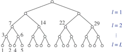
To conveniently organize the FMM matrix representation, we introduce a postordered binary tree T
with nodes i= 1,2, . . . ,root(T), where root(T) denotes the root node. See Figure 1. SupposeT hasL levels such thatn/2L−1=O(r) and root(T) is at level 0. We partition the setshierarchically following
T. That is, suppose each node i is associated with a subsetxi ⊂s so that xroot(T) =s and for any nonleaf nodeiwith childrenc1andc2,
xi=xc1∪xc2, xc1∩xc2 =∅.
Based on the subinterval where x(i) is located, we can conveniently determine a centerz
iand a radius
δi ofxi. For each leaf i, the cardinalitymi≡ |x(i)|=O(r).
1 2 4 5 3 6 7 14 22 29 l = 1 l = L ... l = 2
Fig. 1 Example of a postordered treeT used for the FMM.
Later for convenience, when xi is used, we may simply refer to node i of T. For example, given
two nodes i and j of T corresponding to two separated sets xi and xj (as defined in Definition 1),
respectively, we just sayiandjare separated.
Supposexicorresponds to the index setIiso thatA|Ii×Ij= (κ(xi, xj))xi∈xi,xj∈xj, which is said to
be theinteraction (matrix) betweeniandj. Wheniandjare separated,A|Ii×Ij can be approximated
by a low-rank form like in (17) and is said to be afar-field interaction. For notational convenience, we rewrite (17) as A|Ii×Ij = ˆUiBˆi,jVˆ T j +A|Ii×IjEi,j≈UˆiBˆi,jVˆ T j , (29)
where appropriate sets used for the definition of the matrices in (18) are replaced byxiandxj.
Corre-spondingly, the centerzi, the radiusδi, and the scaling factorsηi,j as in (15) are used for the definition of ˆUi,Bˆi,j,VˆjT in (29).
As mentioned in Remark 1, we say ˆUi the contribution (matrix) from node i. Clearly, ˆUi = ˆVi.
However, to accommodate more general matrix forms, we still use ˆVi for the column basis matrix in
(29).
Wheni andj are not separated, they are said to be near neighbors, and A|I(i)×I(j) is anear-field interaction. Near-field interactions may be further partitioned so as to generate far-field interactions at finer levels.
3.2 Levelwise low-rank approximation
In the FMM, far-field interactions are organized with the aid of interaction lists [13], which illustrate the interactions to consider at each level of partition. Specifically for our case, an interaction list is defined as follows.
Definition 2 Theinteraction list Li for nodeiofT is the set of nodesjsatisfying:
– eachj is at the same level asiin T,
– eachj is well-separated fromi,
– and the parents ofj andiare near neighbors.
Corresponding to level l of T, let A(l) be the submatrix extracted from A by retaining only the blocks A|I(i)×I(j) for all nodesiat levell and j∈ Li and zeroing out other blocks in A. For example,
for l= 1, A(l)= 0 since the two nodes at this level are near neighbors (Figure 1). Forl = 2, the four nodes in Figure 1 have interaction lists as follows:
L7={22,29}, L14={29}, L22={7}, L29={7,14}.
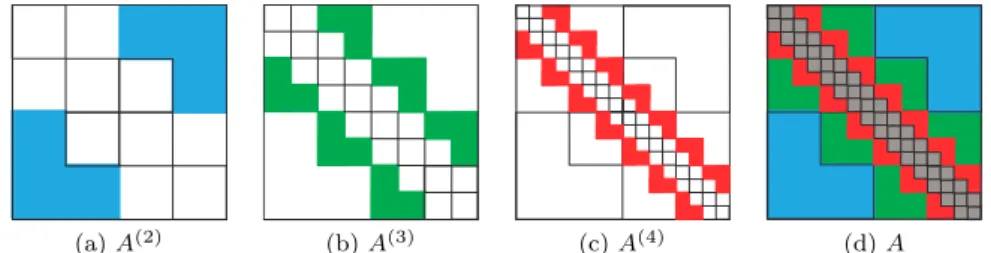
The corresponding far-field interactions are shown in Figure 2(a). Similarly, the far-field interactions for l = 3,4 are shown in Figure 2(b–c). Correspondingly, the matrix A can be decomposed levelwise into the following sum of matrices corresponding to far-field interactions and near-field interactions:
A=A(2)+· · ·+A(L)+A(N), (30) where A(N) denotes all the near-field interactions at the leaf level L of the partition.A(N) is a block banded matrix.
(a)A(2) (b)A(3) (c)A(4) (d)A
Fig. 2 Nonzero patterns ofA(l) and howA(l) appears inA, where the grey band in (d) corresponds toA(N).
For l ≥ 2, the nonzero block A|I(i)×I(j) for each node i at level l and j ∈ Li has a low-rank
approximation as in (29). For convenience, let i1, . . . ,iβ be the nodes at levell ofT, ordered from left to right. Then, we can write
A(l)= ˆU(l)Bˆ(l)( ˆV(l))T+A(l)E(l)≈Uˆ(l)Bˆ(l)( ˆV(l))T, (31) where ˆ U(l)= diag( ˆUi1, . . . ,Uˆiβ), Vˆ (l)= diag( ˆV i1, . . . ,Vˆiβ), (32)
and ˆB(l) and E(l) have the same block nonzero patterns asA(l)with the nonzero blocks A|
I(i)×I(j) of A(l) replaced by ˆBi,j andEi,j, respectively. See Figure 3.
A(l) ~~
=
Fig. 3 Nonzero patterns of ˆU(l), ˆB(l), and ˆV(l) in (31) forA(l)withl= 2 in Figure 2(a).
From (30) and (31), we have the following approximation ofA:
A= L X l=2 ˆ U(l)Bˆ(l)( ˆV(l))T +A(N)+AE (33) ≈ L X l=2 ˆ U(l)Bˆ(l)( ˆV(l))T +A(N)≡A,ˆ
where E=E(2)+· · ·+E(L). Since the nonzero blocks ofE(l) for differentl do not overlap,E satisfies the bound in (28).
Thus, ˆA is an approximation to A with entrywise relative accuracy ε as in (28). It can be easily seen that ˆA can be used to compute matrix-vector products inO(rnL) =O(rnlogn) flops with r=
3.3 Nested basis and FMM matrix in a telescoping expansion form
The essential strategy to reduce the matrix-vector multiplication cost from O(nlogn) to O(n) in the FMM is to use nested basis matrices in the off-diagonal approximations. This can utilize the translation relation in Section 2.3. According to the relation in (25), the basis matrices or contributions from a parent nodeiofT and its childrenc1andc2 are related by
ˆ Ui= ˆ Uc1 ˆ Uc2 ˆ Rc1 ˆ Rc2 , Vˆi= ˆ Vc1 ˆ Vc2 ˆ Wc1 ˆ Wc2 , with (34) ˆ Rc1 = ˆWc1 =Tc1,i, Rˆc2 = ˆWc2 =Tc2,i. (35)
(34) shows how the nested basis matrices are obtained.
Remark 2 Note that the translation relation (24) is a result of the binomial expansion. Although here
c1 andc2 are children ofi, the translation relation in Section 2.3 is not restricted to the case wherec is a child ofi. That is,Tc,iin (26) can be used for any descendantcofi.
The approximation in (33) can then be converted into a nested form via the translation matrices. That is, let
ˆ U(l)= ˆU(l+1)Rˆ(l+1), Vˆ(l)= ˆV(l+1)Wˆ(l+1), l= 1,2, . . . , L−1, (36) where ˆ R(l+1)= diag ˆ Rc1 ˆ Rc2
, c1,c2: children of each nodeiat levell
, ˆ W(l+1)= diag ˆ Wc1 ˆ Wc2
, c1,c2: children of each nodeiat levell
.
We can then rewrite the approximation in (31) as a recursive relation ˆ
U(l)Bˆ(l)( ˆV(l))T = ˆU(L)Rˆ(L−1)· · ·Rˆ(l)Bˆ(l)( ˆW(l))T· · ·( ˆW(L−1))T( ˆV(L))T, (37)
where ˆU(L) and ˆV(L)are defined for the leaf levelLas in (32).
Inserting (37) into (33), we obtain the followingtelescoping expansion of ˆA:
ˆ
A= ˆU(L)Rˆ(L−1) · · ·( ˆR(2)Bˆ(2)( ˆW(2))T + ˆB(3)) (38)
· · ·
( ˆW(L−1))T + ˆB(L)( ˆV(L))T +A(N),
which is the hierarchical matrix form produced by the FMM or theFMM matrix. For convenience, we call the matrices ˆUi,Vˆi,Rˆi,Wˆi,BˆiFMM generators. We also suppose that each nodeiof the FMM tree
T is associated with FMM generators ˆUi,Vˆi,Rˆi,Wˆi,Bˆi. Due to the nested bases, the ˆUi,Vˆi generators
associated with a nonleaf nodei are not explicitly stored. The total storage for the FMM matrix ˆA is then justO(rn). The cost to multiply the FMM matrix and a vector now becomesO(rn).
4 From the FMM matrix to an HSS matrix
We then establish a connection between the FMM matrix ˆAin (38) and an HSS representation. That is, we further write ˆAin an HSS form, which makes it feasible to use fast and stable ULV factorizations for HSS matrices. Note that in other work such as [3, 34, 35], the constructions of HSS matrices are based on algebraic strategies, while here we use an analytical way to convert the FMM matrix to an HSS form. This connection has not been studied before.
4.1 General idea of transforming FMM into HSS matrices
An HSS matrix can be organized with the aid of a binary tree called HSS tree [34]. Here, we can use the same binary treeT like in Figure 1. An HSS form for ˆAcan be defined with the aid of a set ofHSS generators Di, Ui, Vi, Ri, Wi, Bi: ˆ A=Droot(T), Di= Dc1 Uc1Bc1V T c2 Uc2Bc2V T c1 Dc2 , (39) Ui= Uc1 Uc2 Rc1 Rc2 , Vi= Vc1 Vc2 Wc1 Wc2 , (40)
where c1,c2 are the left and right children of a nonleaf nodei, respectively.
Also letIidenote the index set associated withDisuch thatDi= ˆA|Ii×Ii. Then we see from (39)–
(40) that the columns of Uispan the column space of the blockA|Ii×({1:n}\Ii). Similarly, the columns
ofVispan the column space of the block (A|({1:n}\Ii)×Ii)
T. (40) indicates that theU
i, Vibasis matrices
have nested forms so that we only need to storeDi, Ui, Vifor leaf nodesiandRi, Wi, Bifori<root(T).
The HSS form also has a telescoping expansion [21]: ˆ
A=U(L)R(L−1) · · ·(R(2)B(1)(W(2))T +B(2))· · ·
(W(L−1))T +B(L−1) (41)
·(V(L))T+D(L), where
D(L)= diag(Di, i: each node at levelL),
U(L)= diag(Ui, i: each node at levelL),
V(L)= diag(Vi, i: each node at level L),
R(l)= diag
Rc1 Rc2
, c1,c2: children of each nodeiat levell < L
, W(l)= diag Wc1 Wc2
, c1,c2: children of each nodeiat levell < L
, B(l)= diag 0 Bc1 Bc2 0
, c1,c2: children of each nodeiat level l < L
.
The expansion in (41) has a form similar to the telescoping expansion in (38) for the FMM. These two telescoping expansions have the following differences:
– In (38), the last term A(N) for the near-field interactions has a block banded form, while in (41), only the diagonal blocks are considered as near-field interactions so that the last term D(L) has a block diagonal form.
– Accordingly, the ˆU(L), ˆV(L)basis matrices in (38) are different fromU(L),V(L)in (41), respectively, since they are basis matrices for different off-diagonal blocks. ˆR(l), ˆW(l) in (38) are also different fromR(l),W(l) in (41), respectively.
– In (38), ˆB(l) has a block nonzero pattern similar toA(l) illustrated in Figure 2, while in (41),B(l) has a block-diagonal form.
We will resolve these differences by showing how to construct an HSS form from the FMM form. It should be noted that the HSS form we are constructing is for the FMM matrix ˆAin (38). That is, we are constructing an HSS approximation toA.
The basic idea of constructing the HSS form of ˆA is to find HSS representations for the far-field matrix Aˆ(F) ≡ Aˆ−A(N) and the near-field matrix A(N) separately and then to merge the two sets of HSS generators. In Figure 2(d), A(N) corresponds to the grey banded matrix along the diagonal and ˆA(F) corresponds to the remaining part of the matrix. To distinguish the generators for different matrices, we use the following notation.
– U ,ˆ Vˆ, etc.: FMM generators of ˆA(F) from the FMM procedure in Section 3.
– U, V, etc.: HSS generators for the HSS form of ˆA.
– U ,˜ V˜, etc.: HSS generators for the HSS form of ˆA(F).
The HSS representation for the near-field partA(N)can be explicitly written out based on its block banded form. The main task is then to find the HSS representation of the far-field part ˆA(F). We do this in two steps:
1. First, we write each off-diagonal block in a low-rank form ˆ
A(F)|Ii×Ij= ˜UiB˜iV˜
T
j , (42)
whereiandjare sibling nodes inT (i.e.,j= sib(i)) with the corresponding index setsIi andIj in
A, respectively. As in Section 3, we suppose each nodeiis associated with a set of pointsxi∈s.
2. Then we write the ˜U ,V˜ basis matrices in nested forms. That is, we obtain the ˜R,W˜ generators in (40).
The two steps above will be elaborated in Sections 4.2 and 4.3, respectively. The HSS representations for ˆA(F) and ˆA(N) will be merged to form an HSS representation for ˆAin Section 4.4.
4.2 Low-rank forms of off-diagonal blocks of ˆA(F)
For sibling nodesi,jofT, we find the HSS generators ˜Ui,B˜i,V˜j so as to write ˆA(F)|Ii×Ij in the form of
(42).
The FMM procedure yields a partition that accounts for all far-field interactions between subsets of xi and s\xi. Accordingly, Ii is partitioned into subsets following the partitioning of xi. Late for
convenience, we consider the partition of the index set Ii instead of xi. Note that subsets resulting
from the partitioning of Ii correspond to the descendants of the nodei in T. Figure 4 illustrates the
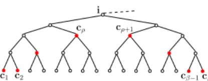
partitioning ofIiand the subsets correspond to the nodes marked in Figure 5. These nodes form a set
which we call thepartition list associated with i.
Definition 3 SupposeT is a postordered full binary tree. Letc1be the smallest labeled leaf descendant of a nodeiandcβ be the largest labeled leaf descendant ofi. LetP1be the set of all the nodes in the path from par(c1) (the parent ofc1) to the left child ofiandP2be the set of all the nodes in the path from par(cβ) to the right child ofi. Then thepartition list associated withiofT is
Ωi={c1} ∪ {the right child of eachj∈ P1} ∪ {the left child of eachj∈ P2} ∪ {cβ}.
Ii
c1c2 · · · cρ cρ+1 · · · cβ
Fig. 4 Partitioning of the index setIiassociated with nodei.
c1 c2
cρ cρ+1
cβ cβ−1 i
Fig. 5 Nodes in the partition listΩi(marked as red solid nodes) corresponding to the partition ofIiin Figure 4.
Thus,Ωi consists of nodesc1 and cβ corresponding to the boundaries ofIi and nodes at levels as
high as possible for the interior subsets ofIi. When we study the interaction betweeniand other nodes,
Ωi is used to provide a way to systematically organize the partition of Ii. The resulting partition like
in Figure 4 is also used in [7].
We then find ˜Ui, ˜Vj, and ˜Bi in (42). The FMM procedure yields a partition ofIi∪ Ij, leading to
a blockwise agglomeration [18] of ˆA(F)|
Ii×Ij. For convenience, suppose Ωi has the following form as
marked in Figures 4–5:
wherecρandcρ+1are the left and right children ofi, respectively. Similarly, supposeΩjhas the following
form:
Ωj={d1,d2, . . . ,dξ,dξ+1, . . . ,dθ}. (44) where dξ anddξ+1 are the left and right children ofj, respectively. As shown in Section 3.1, for each pair of separated sets ci anddj, we can find a low-rank form
ˆ A(F)|Ici×Idj = ˆUci ˆ Bci,djVˆ T dj. (45) Note that ˆA(F)|
Ici×Idj = 0 if ci and dj are near neighbors. In such a case, we can set ˆBci,dj = 0 so that (45) still holds. Then we can assemble all the blocks ˆA(F)|Ici×Idj fori= 1, . . . , β,j= 1, . . . , θinto
˜ UiB˜iV˜jT in (42), where ˜ Ui= diag( ˆUc1, . . . ,Uˆcβ), V˜j= diag( ˆVd1, . . . ,Vˆdθ), (46) ˜ Bi= ˆ Bc1,d1 . . .Bˆc1,dθ .. . · · · ... ˆ Bcβ,d1 . . .Bˆcβ,dθ . (47)
An illustration of (42) with (46)–(47) is shown in Figure 6.
d1 · · · dξ dξ+1 · · · dθ c1 cρ cρ+1 cβ ... ... = U˜i ˜ Bi V˜jT ˆ A(F)| Ii×Ij
Fig. 6 Illustration of (42) with (46)–(47) for the low-rank form of ˆA(F)|
Ii×Ij, wherej= sib(i).
4.3 Nested ˜U ,V˜ basis matrices
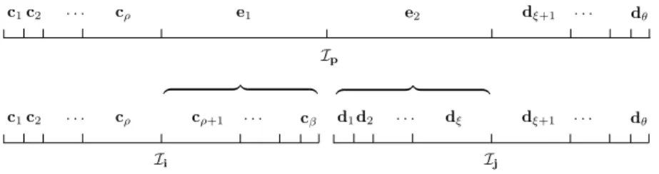
We then derive the nested forms of the basis matrices. Supposeiandjare a pair of sibling nodes with parent p= par(i). Suppose the partition listsΩi andΩj associated withiand j are in (43) and (44),
respectively, which are used for the partitioning of the corresponding index setsIiandIj. Let the index
set associated withpinAbeIp=Ii∪ Ij. Then the partition listΩpassociated withpcan be obtained
by merging and modifying Ωi andΩj. This is illustrated in Figure 7. We can then let
Ωp={c1,c2, . . . ,cρ,e1,e2,dξ+1, . . . ,dθ},
where e1 = par(cρ+1) and e2 = par(dξ). Note that the nodes cρ+1, . . . ,cβ are descendants of e1 and
d1, . . . ,dξ are descendants ofe2. Ii c1c2 · · · cρ cρ+1 · · · cβ Ij d1d2 · · · dξ dξ+1 · · · dθ Ip c1c2 · · · cρ e1 e2 dξ+1 · · · dθ
Like in (46), we have ˜
Up= diag( ˆUc1, . . . ,Uˆcρ,Uˆe1,Uˆe2,Uˆdξ+1, . . . ,Uˆdθ).
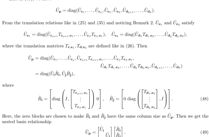
From the translation relations like in (25) and (35) and noticing Remark 2, ˆUe1 and ˆUe2 satisfy ˆ
Ue1= diag( ˆUcρ+1Tcρ+1,e1, . . . ,UˆcβTcβ,e1), Uˆe2= diag( ˆUd1Td1,e2, . . . ,UˆdξTdξ,e2),
where the translation matricesTc,e1, Td,e2 are defined like in (26). Then ˜ Up= diag( ˆUc1, . . . ,Uˆcρ,Uˆcρ+1Tcρ+1,e1, . . . ,UˆcβTcβ,e1, ˆ Ud1Td1,e2, . . . ,UˆdξTdξ,e2,Uˆdξ+1, . . . ,Uˆdθ) = diag( ˜UiR˜i,U˜jR˜j), where ˜ Ri= diag I, Tcρ+1,e1 .. . Tcβ,e1 0 , ˜ Rj= 0 diag Td1,e2 .. . Tdξ,e2 , I . (48)
Here, the zero blocks are chosen to make ˜Riand ˜Rjhave the same column size as ˜Up. Then we get the
nested basis relationship
˜ Up= ˜ Ui ˜ Uj ˜ Ri ˜ Rj . (49)
This yields the nested relation for the ˜U basis matrices. Noticing the pattern of ˜Ui in Figure 6, we
can illustrate the nested basis relation in Figure 8. We can similarly derive a nested basis relationship for ˜Vi. Since the translation matrices only depend on relevant centers of subsets, ˜Ri and ˜Wi are only
determined by the partition ofIiand are independent of the actual points inIi. It follows that the HSS
generator
˜
Wi= ˜Ri. (50)
At this point, we obtain all the ˜U ,V ,˜ R,˜ W ,˜ B˜ generators for ˆA(F). The ˜D generators of ˆA(F) are zero blocks. Clearly, the generators have block structures that can be explored to save storage and computational costs. = ˜ Up ˜ U i ˜ U j ˜ R i ˜ Rj
4.4 HSS representation for ˆA
We then write an HSS representation for A(N) so as to get an HSS form for A = ˆA(F)+A(N). A(N) is a block banded matrix. Suppose A(F)and A(N) are partitioned conformably. Then the HSS form of A(N)can be explicitly written as [32]:
ˇ Ui=I, Vˇi=I, for a leafi, ˇ Ri=
[I 0] ifiis a leaf andi<sib(i), [0 I] ifiis a leaf andi>sib(i),,
diag (I,0), ifiis a nonleaf node andi<sib(i), diag (0, I), ifiis a nonleaf node andi>sib(i), ˇ
Wi: in the same form as ˇRi,
ˇ Bi=
A|Ii×Isib(i), ifiis a leaf andi<sib(i), A|Isib(i)×Ii, ifiis a leaf andi>sib(i), "
0 A|Ii×Isib(i)
#
, ifiis a nonleaf node andi<sib(i),
"
A|Isib(i)×Ii
0
#
, ifiis a nonleaf node andi >sib(i).
(51)
With the HSS generators for A(F) and A(N) at hand, it is easy to verify (see, e.g., [32]) that the HSS generators for ˆA are given by:
Di= ˜Di+ ˇDi, Bi= diag( ˜Bi,Bˇi), Ui= ˜ UiUˇi , Vi= ˜ ViVˇi , (52) Ri= diag( ˜Ri,Rˇi), Wi= diag( ˜Wi,Wˇi).
Due to the summation, the sizes of some generators such asBimay be larger than necessary. If a more
compact HSS form is desired, a recompression step may be applied like in some other HSS methods [9, 12, 33].
5 Stability
Now we would like to illustrate that the structured representations given in the previous sections enable stable computations such as matrix-vector multiplications (with the FMM or HSS form) and ULV factorizations (with the HSS form). The backward stability of several commonly used HSS algorithms has been studied in [7, 30, 31], where the stability analysis essentially relies on the following conditions:
– theU, V generators have bounded norms;
– theB generators have norms bounded by a small constant multiple of the norm ofA.
Thus, our purpose is to show that, the FMM (and HSS generators) we derive using our scaling strategy satisfy such norm requirements. Based on the analysis in Section 2, we have the following bounds for the norms of the generators.
Corollary 1 Suppose (27)holds for any descendantcof a nonleaf nodei inT. Then for the approxi-mation Aˆ toAin (2)with (4), the FMM generatorsU ,ˆ V ,ˆ Bˆ in (18)andR,ˆ Wˆ in (35)satisfy
kUˆkmax≤1, kVˆkmax≤1, kRˆkmax≤1, kWˆkmax≤1,
kBˆkmax≤max{1,3τ}(1 +τ)kAkmax. The HSS generators U, V, R, W, B in (52)satisfy
kUkmax≤1, kVkmax≤1, kRkmax≤1, kWkmax≤1,
Proof The max-norm results for the generators ˆU ,V ,ˆ R,ˆ Wˆ are immediate from Theorems 1 and 2. According to Theorem 1, when ˆA|Ii×Ij= ˆUiBˆi,jVˆ
T
j like in (29) for two separated point setsxi andxj,
we have
kBˆi,jkmax≤max{1,3τ}|κ(z1, z2)|,
wherez1andz2are the centers ofxiandxj, respectively. Due to the separation condition in Definition
1, we have (8) holds for any x∈xiandy∈xj. Thus,
kBˆi,jkmax≤max{1,3τ}(1 +τ)|κ(x, y)| ≤max{1,3τ}(1 +τ)kA|Ii×Ijkmax ≤max{1,3τ}(1 +τ)kAkmax.
Accordingly, the HSS generators ˜B like in (47) also satisfy the bound above.
Next, it is clear from (51) that the HSS generators ˇU ,V ,ˇ R,ˇ Wˇ for ˆA(N)have entrywise magnitudes bounded by 1. Then it can be seen from (52) that the HSS generators U, V, R, W for ˆAhave entrywise magnitudes bounded by 1. Also,
kBkmax≤max{kB˜kmax,kBˇkmax} ≤max{max{1,3τ}(1 +τ)kAkmax,kAkmax}
≤max{1,3τ}(1 +τ)kAkmax. We then get the bound for kBkmax.
Based on these bounds, the stability of various algorithms that use the FMM or HSS forms can then be shown. For example, in the FMM matrix-vector multiplication, the stability of multiplying ˆUBˆVˆT and vectors can be studied as follows.
Theorem 3 Let Kˆ = ˆUBˆVˆT be the approximation to the m×p block K as in (17)–(18). Then the matrix-vector multiplicationˆb= ˆUBˆVˆTw≈Kw for a vectorwsatisfies
fl(ˆb) = ( ˆUBˆVˆT +∆K)w,ˆ with
k∆KˆkF ≤max{1,3τ}(1 +τ)r2
√
mpγp+2rkKkF+O(2mach),
wherefl(·)denotes the numerical result in floating point operations, mach denotes the machine epsilon, andγk =1−kkmachmach.
Proof It is commonly known that (see, e.g., [19]), for a matrixCwith column sizep, the matrix-vector multiplicationCw satisfies the following backward error result:
fl(Cw) = (C+∆C)w, |∆C| ≤γp|C|.
Thus, when we consider the matrix-vector multiplication ˆKw= ˆUBˆVˆTw, we have b1= fl( ˆVTw) = ( ˆVT +∆VˆT)w, |∆VˆT| ≤γp|VˆT|, b2= fl( ˆBb1) = ( ˆB+∆B)bˆ 1, |∆Bˆ| ≤γr|Bˆ|,
ˆb= fl( ˆU b2) = ( ˆU+∆Uˆ)b2, |∆Uˆ| ≤γr|Uˆ|. (Note that ˆKism×pand ˆB is r×r.) Combining these results, we get
fl( ˆUBˆVˆTw) = ( ˆU +∆Uˆ)( ˆB+∆B)( ˆˆ VT +∆VˆT)w≡( ˆUBˆVˆT +∆K)w,ˆ where
k∆KˆkF ≤ kUˆB(∆ˆ VˆT)kF+kUˆ(∆B) ˆˆ VTkF+k(∆Uˆ) ˆBVˆTkF +O(2mach)
≤(γp+ 2γr)kUˆkFkBˆkFkVˆkF+O(2mach).
(Here, we use Frobenius norm in the backward error instead of the max-norm as in Corollary 1 since the former is sub-multiplicative but the latter is not.) According to Corollary 1,
k∆KˆkF ≤(γp+ 2γr) √ mr√rp(max{1,3τ}(1 +τ)rkKkF) +O(2mach) = max{1,3τ}(1 +τ)r2√mp (p+ 2r)mach−3rp 2 mach 1−(p+r)mach+rp2mach kKkF+O(2mach) ≤max{1,3τ}(1 +τ)r2√mpγp+2rkKkF+O(2mach).
This theorem shows the backward stability of using the low-rank approximation ˆKto compute the matrix-vector product ˆKw that approximatesKw. (For this reason, it makes somewhat more sense to use K in the backward error bound.) Stability analysis of the overall FMM algorithm and the HSS matrix-vector multiplication can then be performed similarly to that in [30]. In fact, such stability can be conveniently understood based on the telescoping expansions in (38) and (41). The stability of ULV factorizations and solutions for the HSS form of ˆA can be shown similar to the work in [30, 31]. The actual derivations involve lengthy technical details and thus the readers are referred to [30, 31].
Note that, if no scaling is used as in the standard FMM, thenkUˆkmax,kBˆkmax, and/orkVˆkmaxmay get very large, leading to significantly larger backward error bounds. The impact can be observed from the numerical results in the next section.
6 Performance and tests
6.1 Storage and complexity
We then briefly look at the storage and costs related to the FMM/HSS matrix construction and some FMM/HSS operations. Recall thatn=|s|is the number ofxipoints in (1) that define the kernel matrix A in (2) and is the order of A. ris the number of terms in the truncated expansion (6) and also the order of the ˆBgenerators in (18). Without loss of generality, suppose the partitioning of the pointssas in Section 3.1 is fine enough so thatA(N)has bandwidthO(r) and the FMM tree T hasL=O(logn
r) levels. Also suppose each node at levell corresponds toO(r2L−l+1) points.
Since all the FMM generators can be explicitly written out, the cost to construct the FMM form is mainly for evaluating the entries of the generators. This cost is then proportional to the total storage of those generators. Since the generators associated with each node i needs O(r2) storage, the total storage is
1
X
l=L
O(2lr2) =O(rn).
Thus, the cost to construct the FMM matrix is O(rn). Accordingly, the cost to construct the HSS matrix is alsoO(rn). Then obviously, the cost to multiply the FMM and HSS matrices with a vector is
O(rn).
We then estimate the cost for the ULV factorization of the HSS matrix given by the generators (52). An HSS generatorsBiassociated with nodeiat levellof the HSS tree has orderO((L−l+ 1)r), which
depends on the level l. Following the rank pattern analysis in [33, Theorem 6.1], we can get the ULV factorization cost as 1 X l=L O(2l((L−l+ 1)r)3) =O(r2n). 6.2 Numerical tests
Here, we use some numerical examples to demonstrate the performance of our techniques and support the analysis. We show how our stable FMM/HSS constructions with the scaling strategy control the norms of the generators and the approximation accuracy. We also test the accuracy of direct solution. Different types of kernels as follows are tested:
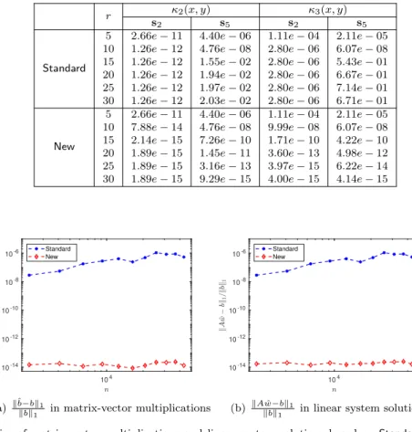
κ1(x, y) = 1 x−y,ifx6=y, 1, otherwise, (53) κ2(x, y) = 1 (x−y)2,ifx6=y, 1, otherwise, κ3(x, y) = log|x−y|,ifx6=y, 1, otherwise. (54)
To account for factors like the scale and distribution of point sets, the kernels are evaluated at various 1D and 2D point sets.
– Sets1: A set of uniform grid points in [0,1].
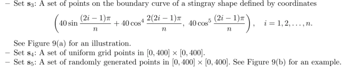
– Sets3: A set of points on the boundary curve of a stingray shape defined by coordinates 40 sin(2i−1)π n + 40 cos 42(2i−1)π n , 40 cos 5(2i−1)π n , i= 1,2, . . . , n.
See Figure 9(a) for an illustration.
– Sets4: A set of uniform grid points in [0,400]×[0,400].
– Sets5: A set of randomly generated points in [0,400]×[0,400]. See Figure 9(b) for an example.
-40 -20 0 20 40 60 80 -40 -30 -20 -10 0 10 20 30 40 0 100 200 300 400 0 50 100 150 200 250 300 350 400 (a)s3 (b)s5
Fig. 9 Illustration of points in examples ofs3 ands5.
To generate a binary treeT for the FMM/HSS matrix construction, we hierarchically bisect each set. Separated subsets are adaptively identified in the partitioning process.
6.2.1 Entrywise magnitudes of generators
We illustrate the benefit of the proposed stable FMM/HSS matrix construction by investigating the entrywise magnitudes of the generators with and without applying the scaling strategy (denoted New
and Standardin the tests, respectively). According to (52) and Corollary 1, we just need to report the entrywise magnitudes for the HSS version since the results are almost the same for the FMM case. To inspect how New differs fromStandard, we report the entrywise magnitudes of the HSS generators of
ˆ A(F) as follows: B ≡max i∈T k ˜ Bikmax, U ≡max i∈T k ˜ Uikmax, R ≡max i∈T k ˜ Rikmax. (55)
Results for the generators ˜V and ˜W are not shown since they are similar to those for ˜U and ˜R, respectively.
We pick the number of points in each point set (or the order of A) as n= 4096 and set each leaf level partition to include at most 256 points. The separation ration τ in Definition 1 is set to be 12 for sets s1,s2and
√ 2
2 fors3,s4,s5. The number of expansion termsrincreases from 5 to 30 so as to show how the standard Taylor series expansion leads to large entrywise magnitudes of the generators.
For the kernelκ1(x, y) in (53), the results on the maximum entrywise magnitudes (55) are given in Tables 1 and 2. As rincreases, the maximum entrywise magnitudes of some generators fromStandard
get quite large. For some cases, even a small increase in r leads to a rapid increase in the entrywise magnitudes and the magnitudes become significantly larger thankAkmax. Such large magnitudes occur in different generators, depending on the point set. On the other hand,Newfully resolves this issue and produces generators with uniformly bounded matrix entries regardless of the scale and the distribution of the point sets. That is, allU,Rare bounded by 1, which is consistent with Corollary 1. TheBvalues are also bounded by modest constants.
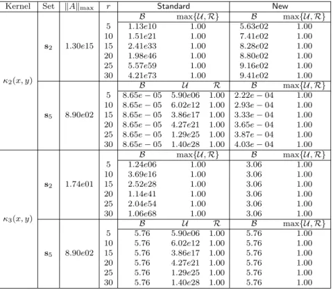
Similar results can also observed for other kernel functions. We repeat some tests with the ker-nels κ2(x, y) and κ3(x, y) in (54). The results are shown in Table 3. Again, while some generators from Standard have large magnitudes, the generators from New always have well-controlled entrywise magnitudes.
Other than increasing r, another way to demonstrate the advantage of New over Standard is to increase the number of points nin a set while keeping the points still within the given interval. In this way, the points get more clustered and the entries in (10) and (13) used in Standard get larger. For
Table 1 Maximum entrywise magnitudes of the HSS generators of ˆA(F) obtained withStandardand Newforκ 1(x, y)
discretized on the setss1,s2.
Set kAkmax r B Standard New
max{U,R} B max{U,R} s1 4.10e3 5 1.04e05 1.00 5.33e00 1.00 10 6.77e12 1.00 5.33e00 1.00 15 7.03e21 1.00 5.33e00 1.00 20 4.24e31 1.00 5.33e00 1.00 25 9.34e41 1.00 5.33e00 1.00 30 5.75e52 1.00 5.33e00 1.00 s2 3.60e7 5 1.06e08 1.00 2.13e01 1.00 10 7.09e18 1.00 2.13e01 1.00 15 7.52e30 1.00 2.13e01 1.00 20 4.64e43 1.00 2.13e01 1.00 25 1.05e57 1.00 2.13e01 1.00 30 6.58e70 1.00 2.13e01 1.00
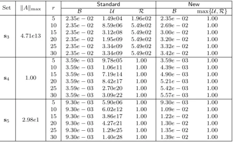
Table 2 Maximum entrywise magnitudes of the HSS generators of ˆA(F) obtained withStandardand Newforκ
1(x, y)
discretized on the setss3,s4,s5.
Set kAkmax r Standard New
B U R B max{U,R} s3 4.71e13 5 2.35e−02 1.49e04 1.96e02 2.35e−02 1.00 10 2.35e−02 8.59e06 5.49e02 2.69e−02 1.00 15 2.35e−02 3.12e08 5.49e02 3.00e−02 1.00 20 2.35e−02 1.95e09 5.49e02 3.20e−02 1.00 25 2.35e−02 3.34e09 5.49e02 3.32e−02 1.00 30 2.35e−02 3.34e09 5.49e02 3.42e−02 1.00 s4 1.00 5 3.59e−03 9.78e05 1.00 3.59e−03 1.00 10 3.59e−03 1.06e11 1.00 4.39e−03 1.00 15 3.59e−03 7.19e14 1.00 4.90e−03 1.00 20 3.59e−03 8.42e17 1.00 5.21e−03 1.00 25 3.59e−03 2.70e20 1.00 5.42e−03 1.00 30 3.59e−03 3.09e22 1.00 5.57e−03 1.00 s5 2.98e1 5 9.30e−03 5.90e06 1.00 9.30e−03 1.00 10 9.30e−03 6.02e12 1.00 1.09e−02 1.00 15 9.30e−03 3.86e17 1.00 1.22e−02 1.00 20 9.30e−03 4.27e21 1.00 1.30e−02 1.00 25 9.30e−03 1.29e25 1.00 1.35e−02 1.00 30 9.30e−03 1.40e28 1.00 1.39e−02 1.00
example, for κ1(x, y) discretized on s2, we fix r = 20 and increase n. The B magnitudes are plotted in Figure 10. It can be observed that Bfrom Standard increases quickly with n, while it remains well bounded from New. We can observe similar comparisons for the other sets and kernels.
104 100 1020 1040 1060 1080 Standard New
Fig. 10 Maximum entrywise magnitudeB in (55) fromStandardandNew for ˆA(F) withκ
1(x, y) discretized on s2 of
Table 3 Maximum entrywise magnitudes of the HSS generators of ˆA(F)obtained withStandardandNewfor the kernels
in (54) discretized on the setss2,s5.
Kernel Set kAkmax r Standard New
κ2(x, y) B max{U,R} B max{U,R} 5 1.13e10 1.00 5.63e02 1.00 10 1.51e21 1.00 7.41e02 1.00 s2 1.30e15 15 2.41e33 1.00 8.28e02 1.00 20 1.98e46 1.00 8.80e02 1.00 25 5.57e59 1.00 9.16e02 1.00 30 4.21e73 1.00 9.41e02 1.00 B U R B max{U,R} 5 8.65e−05 5.90e06 1.00 2.22e−04 1.00 10 8.65e−05 6.02e12 1.00 2.93e−04 1.00 s5 8.90e02 15 8.65e−05 3.86e17 1.00 3.33e−04 1.00 20 8.65e−05 4.27e21 1.00 3.65e−04 1.00 25 8.65e−05 1.29e25 1.00 3.87e−04 1.00 30 8.65e−05 1.40e28 1.00 4.03e−04 1.00 κ3(x, y) B max{U,R} B max{U,R} 5 1.24e06 1.00 3.06 1.00 10 3.69e16 1.00 3.06 1.00 s2 1.74e01 15 2.52e28 1.00 3.06 1.00 20 1.14e41 1.00 3.06 1.00 25 2.04e54 1.00 3.06 1.00 30 1.06e68 1.00 3.06 1.00 B U R B max{U,R} 5 5.76 5.90e06 1.00 5.76 1.00 10 5.76 6.02e12 1.00 5.76 1.00 s5 8.90e02 15 5.76 3.86e17 1.00 5.76 1.00 20 5.76 4.27e21 1.00 5.76 1.00 25 5.76 1.29e25 1.00 5.76 1.00 30 5.76 1.40e28 1.00 5.76 1.00
Remark 3 In practice, even ifris very small (say, smaller than 10),Standardmay still provide generators with huge entries that pose stability risks. Also, we have used computational domains with different sizes to show thatStandardis susceptible to problem settings butNewis much more robust.
6.2.2 Accuracy and efficiency
The large magnitudes of the entries of the generators can cause accuracy loss to structured algorithms using the generators. To demonstrate this, we perform some operations on the generators in (52). The recompression step mentioned after (52) is first applied with the full machine precision as the tolerance so as to avoid introducing extra approximation errors. The resulting generators are used for matrix-vector multiplications and linear system solutions via ULV factorizations and solutions.
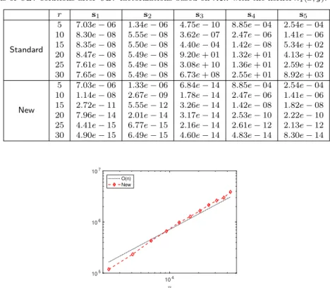
For each matrix-vector multiplication, we generate a random vectorwand multiply the approximate matrix withwto get a vector ˆb, which approximates the exact vectorb=Aw. Forκ1(x, y) discretized on the point sets as above, the resulting matrix-vector multiplication errors kˆbk−bk1bk1 are shown in Table 4. In exact arithmetic, when r increases, the approximate matrix gets more accurate and the error
kˆb−bk 1
kbk1 should decreases. However, withStandard, only modest accuracies are achieved. Specifically for the sets s1,s2, the accuracy in Table 4 does not improve much for increasingr. For the setss3,s4,s5, the accuracy in Table 4 initially improves with increasingrbut then decreases. On the other hand, such situations do not occur with New. For all the sets, the accuracy increases with r to near the machine precision.
For the kernelsκ2(x, y) andκ3(x, y), the results are given in Table 5.
We then fix r = 20 and increase n. Figure 11(a) shows the relative errors of the matrix-vector multiplications for one case. Much higher accuracies are achieved for allnwithNewthan withStandard. We can similarly compare the accuracies in linear system solution with ULV factorization and ULV solution. We form the right-hand side vectorb=Awwith randomwand suppose ˆwis the approximate solution. Forκ1(x, y) discretized on the five sets as above, Table 6 gives the relative residuals k
Awˆ−bk1 kbk1 . WithStandard, only modest accuracies can be achieved for some cases and very inaccurate results are
Table 4 kˆb−bk1
kbk1 : accuracy of matrix-vector multiplications based onStandardandNewwith the kernelκ1(x, y).
r s1 s2 s3 s4 s5 Standard 5 7.03e−06 1.34e−06 4.13e−13 1.11e−04 1.20e−04 10 8.30e−08 5.55e−08 1.50e−10 6.32e−07 6.93e−07 15 8.35e−08 5.50e−08 1.05e−08 7.18e−09 1.98e−01 20 8.47e−08 5.49e−08 7.24e−06 2.95e−01 2.62e−01 25 7.61e−08 5.49e−08 9.78e−02 3.21e−01 2.91e−01 30 7.65e−08 5.49e−08 2.13e−01 3.25e−01 2.99e−01 New 5 7.03e−06 1.33e−06 1.33e−06 1.11e−04 1.20e−04 10 1.14e−08 2.67e−09 2.67e−09 6.32e−07 6.93e−07 15 2.72e−11 5.55e−12 5.55e−12 7.18e−09 7.20e−09 20 7.84e−14 1.81e−14 1.81e−14 9.93e−11 1.08e−10 25 1.62e−15 1.83e−15 1.83e−15 1.76e−12 1.92e−12 30 1.54e−15 1.81e−15 1.81e−15 3.49e−14 4.17e−14 Table 5 kˆb−bk1
kbk1 : accuracy of matrix-vector multiplications based onStandardand New with the kernelsκ2(x, y) and
κ3(x, y). r κ2(x, y) κ3(x, y) s2 s5 s2 s5 Standard 5 2.66e−11 4.40e−06 1.11e−04 2.11e−05 10 1.26e−12 4.76e−08 2.80e−06 6.07e−08 15 1.26e−12 1.55e−02 2.80e−06 5.43e−01 20 1.26e−12 1.94e−02 2.80e−06 6.67e−01 25 1.26e−12 1.97e−02 2.80e−06 7.14e−01 30 1.26e−12 2.03e−02 2.80e−06 6.71e−01 New 5 2.66e−11 4.40e−06 1.11e−04 2.11e−05 10 7.88e−14 4.76e−08 9.99e−08 6.07e−08 15 2.14e−15 7.26e−10 1.71e−10 4.22e−10 20 1.89e−15 1.45e−11 3.60e−13 4.98e−12 25 1.89e−15 3.16e−13 3.97e−15 6.22e−14 30 1.89e−15 9.29e−15 4.00e−15 4.14e−15 104 10-14 10-12 10-10 10-8 10-6 Standard New 104 10-14 10-12 10-10 10-8 10-6 Standard New (a) kˆb−bk1 kbk1 in matrix-vector multiplications (b) kAwˆ−bk1
kbk1 in linear system solutions
Fig. 11 Accuracies of matrix-vector multiplications and linear system solutions based onStandardand Newwith the
kernelκ1(x, y) discretized ons2 of different sizen.
produced for the other cases. With New, the relative residuals reduce with increasing r to near the machine precision.
Similarly, with r = 20 and varying n, the accuracy results for one test is given in Figure 11(b). While the accuracy with Standardremains modest and gets worse with increasingn, the accuracy with
New stays high for all thenvalues.
Finally, it is convenient to check the efficiency of relevant structured algorithms. Such efficiency studies have been done extensively in many existing literatures. Here, we just use Figure 12 withr= 20 to show the storage needed for the generators for ˆA(F), which essentially reflects the cost needed to multiply ˆA(F) with a vector. The storage in Figure 12 is roughly linear inn.
Table 6 Residuals of ULV solutions after ULV factorizations based onNewwith the kernelκ1(x, y). r s1 s2 s3 s4 s5 Standard 5 7.03e−06 1.34e−06 4.75e−10 8.85e−04 2.54e−04 10 8.30e−08 5.55e−08 3.62e−07 2.47e−06 1.41e−06 15 8.35e−08 5.50e−08 4.40e−04 1.42e−08 5.34e+ 02 20 8.47e−08 5.49e−08 9.20e+ 01 1.32e+ 01 4.13e+ 02 25 7.61e−08 5.49e−08 3.08e+ 10 1.36e+ 01 2.59e+ 02 30 7.65e−08 5.49e−08 6.73e+ 08 2.55e+ 01 8.92e+ 03 New 5 7.03e−06 1.33e−06 6.84e−14 8.85e−04 2.54e−04 10 1.14e−08 2.67e−09 1.78e−14 2.47e−06 1.41e−06 15 2.72e−11 5.55e−12 3.26e−14 1.42e−08 1.82e−08 20 7.96e−14 2.01e−14 3.17e−14 2.53e−10 2.22e−10 25 4.41e−15 6.77e−15 2.16e−14 2.61e−12 2.13e−12 30 4.90e−15 6.49e−15 4.60e−14 4.83e−14 8.30e−14 104 105 106 107 O(n) New
Fig. 12 Storage (number of nonzero entries) for the ˜D,U ,˜ V ,˜ R,˜ W ,˜ B˜generators for ˆA(F)fromNewforκ
1(x, y) discretized
ons2with different number of pointsn.
7 Conclusions
In this paper, stabilization strategies and backward stability studies are given for relevant low-rank approximations and translation relations in an intuitive matrix version of the FMM. An FMM matrix example is also shown, followed by ideas to convert the FMM matrix into an HSS form that admits stable factorizations. The stable matrix version FMM employs a scaling strategy to revise the low-rank approximations based on Taylor expansions for some kernel functions. Rigorous norm bounds are shown for the revised low-rank forms as well as the translation matrices in the FMM. These bounds lead to the backward stability of fast matrix-vector multiplications with the FMM. We also show how to writing an HSS form from an FMM matrix without using explicit compression in previous HSS methods. The HSS form can be used for stable linear system solution via ULV factorization and solution.
Since the approximation based on Taylor expansions can be substituted by other approximations such as polynomial interpolations [11, 16, 36], numerical integrations [1, 37], kernel independent FMM [23, 38, 39], etc., our ideas can also be generalized to various other types of FMM. Our stabilization strategies are derived based on 2D point sets, but can also be extended to higher dimensions. It is convenient to generalize the norm bounds and stability analysis in Sections 2 and 5. Although we only give the FMM matrix using one-dimensional sets as an example, the essential ideas can be directly modified for higher dimensions. Some details will appear in [24].
References
1. Anderson, C.R.: An implementation of the fast multipole method without multipoles. SIAM J. Sci. Stat. Comput.
13, 923–947 (1992)
2. B¨orm, S., Grasedyck L., Hackbusch W.: Introduction to hierarchical matrices with applications. Engineering analysis with boundary elements27, 405–422 (2003)
3. Cai, D., Chow, E., Erlandson, L., Saad, Y., Xi, Y.: SMASH: Structured matrix approximation by separation and hierarchy. Numer. Linear Algebra Appl.25, (2018)
4. Cai D., Xia J.: A stable and efficient matrix version of the fast multipole method. Preprint, https://www.math.purdue.edu/˜cai92/fmm2hss.pdf.
5. Chandrasekaran, S., Dewilde, P., Gu, M., Lyons, W., Pals, T.: A fast solver for hss representations via sparse matrices. SIAM J. Matrix Anal. Appl.29, 67–81 (2007)