Article
A Comparative Study of Water Indexes and Image
Classification Algorithms for Mapping Inland
Surface Water Bodies Using Landsat Imagery
Feifei Pan 1,*, Xiaohuan Xi 2 and Cheng Wang 2
1 Department of Geography and the Environment, University of North Texas, Denton, TX 76203, USA; 2 Key Laboratory of Digital Earth, Institute of Remote Sensing and Digital Earth, Chinese Academy of
Sciences, Beijing 100094, China; [email protected] (X. Xi); [email protected] (C. Wang) * Correspondence: [email protected] (F. Pan); Tel.: +01-940-369-5109
Abstract: To address three important issues related to extraction of water features from Landsat imagery, i.e., selection of water indexes and classification algorithms for image classification, collection of ground truth data for accuracy assessment, this study applied four sets (ultra-blue, blue, green, and red light based) of water indexes (NWDI, MNDWI, MNDWI2, AWEIns, and AWEIs)
combined with three types of image classification methods (zero-water index threshold, Otsu, and kNN) to 24 selected lakes across the globe to extract water features from Landsat-8 OLI imagery. 1440 (4x5x3x24) image classification results were compared with the extracted water features from high resolution Google Earth images with the same (or 1 day) acquisition dates through computing the Kappa coefficients. Results show the kNN method is better than the Otsu method, and the Otsu method is better than the zero-water index threshold method. If the computational cost is not an issue, the kNN method combined with the ultra-blue light based AWEIns is the best method for
extracting water features from Landsat imagery because it produced the highest Kappa coefficients. If the computational cost is taken into account, the Otsu method is a good choice. AWEIns and AWEIs
are better than NDWI, MNDWI and MNDWI2. AWEIns works better than AWEIs under the Otsu
method, and the average rank of the image classification accuracy from high to low is the ultra-blue, blue, green, and red light-based AWEIns.
Keywords: Landsat; Google Earth; water index; unsupervised image classification; supervised image classification; Kappa coefficient
1. Introduction
The Earth’s inland surface water body consists of rivers, freshwater or saltwater lakes, and
marshes with a total surface area of about 5.6 million km2(about 1.1% of Earth’s surface area), i.e.,
0.8 million km2 for rivers [1], 2.1 million km2 for lakes and 2.7 million km2 for marshes [Error! Reference source not found.]. Although these inland surface water bodies only hold about 0.013%
of Earth’s total water, i.e., about 178,000 km3 [2-4], they are important compartments in the global
terrestrial water cycle and mapping inundation areas of inland surface water bodies is of great significance for flood prediction and prevention [5-8], flood risk and damage assessments [9-17], estimation of water storage in rivers, lakes and reservoirs [18-20], calculation of evaporation from wetlands and lakes/reservoirs [21], retrieval of lake water level and river stage [22-25], reservoir operation and management [26], and assessment of ecological functions and health in wetlands and marshes [27,28]. In addition to the above mentioned practical applications, surveying inland surface water body can provide critical measurements/observations for improving our understanding of the water cycle and inundation dynamics at multiple spatial and temporal scales [29-31]. Given the
tremendous surface area associated with the Earth’s inland surface water bodies, mapping their
inundation areas from space using remote sensing technique is indeed one of the most efficient approaches.
Both optical (passive) and microwave (active) remote sensing methods have been widely
utilized for surveying Earth’s inland surface water bodies, but both of them have some advantages and limitations. Microwave remote sensing is not limited by clouds, weather conditions and sunlight, but it usually has coarse spatial resolutions, and revisit frequency is also low. Optical remote sensing of inundation areas only works under clear sky and daylight conditions, while the spatial resolutions of spaceborne optical sensors, especially those mounted on commercial satellites (e.g., Ikonos, QuickBird, WorldView, GeoEye) could achieve the centimeter-level resolutions. Since commercial satellite imagery is not free to public and acquired only through purchase, the most commonly used optical remote sensing images employed for mapping inland surface water bodies at medium resolution (e.g., 30 m) have been and will continually be collected by the Landsat series satellites (e.g., Landsat 4-5 TM, Landsat 7 ETM+, Landsat 8 OLI).
Most researches related to mapping inland surface water bodies using Landsat imagery consist three steps: 1) using the spectral reflectance captured by Landsat to compute one type of water index at each pixel; 2) using one type of image classification algorithm (unsupervised or supervised) to identify water and non-water pixels; 3) using ground truth or alternative data to assess accuracy of the extracted water body features. However, all these three steps have some unsolved issues, and inconsistent conclusions can be found across the literature [32-37]. Therefore, this study is dedicated to address these problems so that our knowledge and techniques in optical remote sensing of inland surface water bodies using Landsat imagery could be advanced.
A number of field experiments measuring various land surface features’ spectral reflectance [38-40] show that turbid water and algae-laden water usually have a distinct higher reflectance in the green light than any other visible lights, and beyond the near-infrared (>0.9m) their spectral
reflectance approaches to zero, unlike soil and vegetation which exhibit high reflectance in infrared bands. The characteristics of water spectral reflectance have promoted three commonly used water indexes developed in the literature: 1) normalized difference water index (NDWI) [41], 2) modified
normalized difference water index (MNDWI) [42], and 3) automated water extraction index (AWEI) [43]. All these three water indexes were derived based on spectral reflectance in the green light and
near-infrared, or shortwave infrared. The NDWI [41] is defined as follows:
𝑁𝐷𝑊𝐼 =𝑅𝑔−𝑅𝑁𝐼𝑅
𝑅𝑔+𝑅𝑁𝐼𝑅 (1)
where Rg and RNIR are spectral reflectance in the green light band and the near-infrared band,
respectively. Xu (2006) showed that the NDWI had troubles to eliminate the build-up land noise from the extracted water features. Considering that the build-up land shows relatively high reflectance in
the shortwave infrared (1.5-3.0m) band than the near-infrared (0.7-1.3 m) band, Xu (2006) modified the NDWI by replacing the near infrared band by the shortwave infrared (SIR) band in the water index referred as the modified normalized difference water index (MNDWI):
𝑀𝑁𝐷𝑊𝐼 =𝑅𝑔−𝑅𝑆𝐼𝑅
𝑅𝑔+𝑅𝑆𝐼𝑅 (2)
Although Landsat-5 TM has two SIR bands (i.e., band 5 and band 7), Xu (2006) found band 5 of Lansdat-5 was better than band 7 and thus band 5 was used in the MNDWI.
In the water body classification, shadows produced by mountains, tree and building, and even river banks can contaminate satellite imagery classification of water features. To remove the impact
of shadows, Feyisa et al. (2014) proposed the AWEI using five bands given as follows:
𝐴𝑊𝐸𝐼𝑛𝑠= 4(𝑅𝑔− 𝑅𝑆𝐼𝑅1) − (0.25𝑅𝑁𝐼𝑅+ 2.75𝑅𝑆𝐼𝑅2) (3)
and
where Rb, Rg, RNIR, RSIR1, and RSIR2 are spectral reflectance in blue light, green light, near infrared,
shortwave infrared 1, and shortwave infrared 2, respectively. To use the AWEI, Feyisa et al. (2014)
suggested the following criteria: 1) for the areas without high albedo surfaces such as snow cover and shadows are the main factor causing errors in the extracted water bodies, AWEIs alone is sufficient to
identify water, 2) if there is no any shadow, SWEIns alone is sufficient, 3) if both high albedo surfaces
and shadow/dark surfaces are present, Eq.(3) and Eq.(4) are used sequentially, 4) without any shadow/dark surfaces and high albedo surfaces, either one alone can be used.
According to Eqs.(1)-(4), not surprisingly, we can find that the spectral reflectance in green light is the key variable in these three commonly used water indexes, given the relatively high reflectance
in green light associated with turbid or algae-laden water measured in the fields [38,39]. Thus in this paper we refer these three commonly used water indexes as the green-light-based water indexes.
However, if we pay attention to the measured spectral reflectance of clear water in Meaden and Kapetsky (1991), we can find that the reflectance in blue light actually is the highest among all visible
lights. On the other hand, if water contains a certain amount of sediments, the spectral reflectance in red light should be the highest [38]. It seems that these kinds of questions have not been paid much attention in the literature, therefore the first goal of this study is to evaluate performances of all water
indexes including the green light- (commonly used), blue light- (only Landsat 8 has this ultra-blue band), ultra-blue light-, and red light- based water indexes.
One key purpose of utilizing water indexes in the extraction of water features from satellite imagery is to simplify the image classification by defining zero water index value as the threshold
to differentiate water and non-water pixels. However, this single zero-water index threshold method may not work well and studies showed a dynamic or automatic selected threshold method such as the Otsu method [43] was better than the zero-water index threshold method [32]. No matter the
single threshold method or the automatic selected threshold method, they all belong to the unsupervised image classification. Compared to the unsupervised image classification, the
supervised image classification should perform better because human intervene and input of training data could assist computers to identify water and non-water pixels, although computational
efficiency of the supervised methods is usually lower than the unsurprised methods. Obviously there is a tradeoff between computational efficiency and accuracy of image classification, and thus the
following questions such as 1) What image classification algorithm is proper for a particular study? 2) How to choose an image classification method? should be answered. Therefore, the second goal of
this study is to address these questions, and provide recommendations regarding selection of image classification methods through comparing performances of different image classification methods. Accuracy assessment is the critical final step in the image classification which also have some
critical issues, such as 1) how to collect ground truth data to validate the image classification results? 2) how to properly compare the computed accuracy (e.g., the Kappa coefficient) among tested sites?
Collecting ground truth data for validating extracted water features from Landsat imagery is time consuming and labor intensive, especially to draw a general conclusion, multiple Landsat images
across the globe are necessary for the accuracy assessment, which make it even more difficult to facilitate a ground campaign to collect all ground truth data for validating all the selected Landsat
Earth and utilized the Google Earth imagery as the “alternative” ground truth data for evaluating
Landsat imagery classification results.
In this paper, we target at these three critical issues and conduct a systematic study to shed new light on the problems and provide our recommendations for the remote sensing community with regrade to the best water index(es) and image classification method(s) in terms of the accuracy of
extracted water features from Landsat imagery. The reminder of this paper is organized into four sections: Section 2 describes study area and data sources. Section 3 introduces the methods employed
in this study. Results and discussion are presented in Section 4. Conclusions are given in Section 5.
2. Study Areas and Data
Unlike Landsat that has a 16-day revisit frequency, high resolution satellites (e.g., Ikonos,
QuickBird, WorldView, GeoEye) seldom continuously scan the Earth as they are overhead, because they are commercial satellites, and high resolution satellite images are only acquired by these
satellites through purchase. Therefore, the number of high resolution satellite images archived in the Google Earth generally is much less than the number of Landsat images over a specified area. To
match the image acquisition date between Landsat imagery and high resolution satellite imagery over a particular water body (such as lakes, rivers), manually searching high resolution satellite
images archived in the Google Earth and Landsat imagery is needed. The strategy taken in this study
is to first find high resolution satellite imagery (click “Show historical imagery” on the Google Earth
top button) over a selected lake, then go to the United States Geological Survey (USGS) EarthExplorer website (earthexplorer.usgs.gov) to search if around the same date (1 day) there is a Landsat image without cloud cover over the selected lake. If a pair of Landsat and Google Earth
images with the same (or ± 1 day) acquisition date are found, the following steps are taken to build the ground truth data based on the Google Earth image.
Step 1: in Google Earth Pro Preferences, select “Decimal Degrees” for “Show Lat/Long”, and “Meters, Kilometers” for “Units of Measurements”.
Step 2: turn on “Show historical imagery” and “Save image”, write a description about the image
and image acquisition date in the “Edit: Title and Description” window.
Step 3: zoom the image to the level as the scale bar showing 1 km. This step can ensure that after reprojection of the Google Earth image from the geographic projection to the Universal Transverse
Mercator (UTM) projection the image spatial resolution is finer than 5 m.
Step 4: press the letter “r” on the keyboard to straighten the view, and from the “View” menu select “Enter Full Screen”.
Step 5: to import the Google Earth image to ArcMap and complete a geo-registration, four control points usually are needed, which usually are chosen at four corners of the image, i.e.,
top-left, top-right, bottom-top-left, and bottom-right. Click on the “Add Placemark” button to add a
placemark, chose the icon “⨀”. Move the icon to one of four corners, and name it to be one of four
corners, and save the latitude and longitude of each corner.
Step 6: click “Save Image” button to save the image.
Step 7: import the Google Earth image to ArcMap, select World WGS84 for the Geographic Coordinate Systems. Use the saved four corners of the Google Earth image to complete a
Step 8: re-project the Google Earth image from the geographic projection to the UTM projection to match the projection of the corresponding Landsat image.
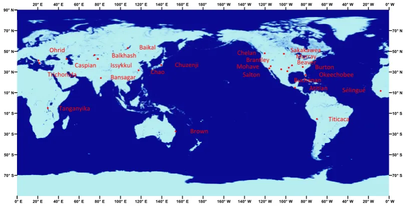
This study selected 24 lakes across the globe as shown in Figure 1. The acquisition date, pixel cell size, water surface elevation (WSE), latitude range and longitude range of each Google Earth image are listed in Table 1, along with the acquisition date, and path and row indexes of the
corresponding Landsat-8 OLI scene downloaded from the USGS EarthExplorer website. For each Landsat-8 OLI scene, first 8 bands (i.e., band 1 - band 8, Table 2 lists Landsat-8 OLI band information)
images were clipped into the same spatial extend as the corresponding Google Earth image, and then resampled into the same spatial resolution as the Google Earth image using the bilinear resampling
method embedded in ArcGIS software package.
Figure 1. Geographic locations of 24 selected lakes across the globe.
Among the downloaded Landsat-8 OLI images in eight bands, band 8 image was only used for correcting the possible errors in the geo-registration of the Google Earth image. Two steps were taken
in this study to reduce such errors: 1) first through a visual inspection to identify a couple of benchmark pixels in both Google Earth image and resampled (i.e., with the same pixel cell size as the
corresponding Google Earth image) Landsat-8 OLI band 8 image, and then determine the average shift in the pixel distance, and apply the average pixel shift distance to correct the Google Earth image; 2) through computing the spatial correlation between the Google Earth image and the resampled
Landsat-8 OLI band 8 image over a range of shift in x and y directions to determine the optimal shift in x and y directions that is associated with the maximum spatial correlation coefficient. Then use the
optimal shift to correct the Google Earth image.
3. Methods
3.1. Water index
As discussed in the Introduction Section, the commonly used water indexes are referred as the green-light-based water indexes. In this study, in addition to these green-light based water indexes,
To compute water indexes, digital number (DN) of each Landsat-8 imagery pixel needs to be converted to the top-of-atmosphere (TOA) spectral reflectance R as follows:
Rλ= (DNλ× M + A)/cosθ (5)
where M = 2 × 10⁻⁵, A=-0.1 are rescaling factors for converting digital number to reflectance in band λ, and θ is the solar zenith angle in degree which is given in the metadata file of each Landsat scene.
Table 1. Characteristics of 24 selected Google Earth and Landsat-8 images
Site Google Earth Landsat-8
Date Cell WSE* Latitude Range Longitude Range Date Path Row Atitlan 2013/12/04 3.5m 1558m 14.7274-14.7590°N 91.1405-91.1855°W 2013/12/04 20 50 Baikal 2013/07/22 4.0m 450m 53.0140-53.0593°N 107.0193-107.1232°E 2013/07/21 133 23 Balkhash 2014/10/10 4.0m 338m 46.3157-46.3551°N 74.8289-74.9075°E 2014/10/10 151 28 Bansagar 2014/02/20 3.5m 324m 24.0759-24.1072°N 80.9680-81.0148°E 2014/02/20 143 43 Beaver 2014/03/19 2.0m 336m 36.3524-36.3667°N 93.9478-93.9707°W 2014/03/20 26 35 Brantley 2016/03/12 3.0m 983m 32.5583-32.5811°N 104.3742-104.4090°W 2016/03/12 31 37 Brown 2016/04/19 2.0m 56m 27.4832-27.4978°S 153.4223-153.4450°E 2016/04/19 89 79 Buchanan 2014/01/13 4.0m 304m 30.7729-30.8028°N 98.4219-98.4667°W 2014/01/13 28 39 Burton 2014/10/22 3.0m 569m 34.8247-34.8504°N 83.5408-83.5842°W 2014/10/22 18 36 Caspian 2016/08/03 3.5m -29m 42.5993-42.6273°N 47.7777-47.8241°E 2016/08/03 168 30 Chao 2017/07/27 3.0m 5m 31.5708-31.5945°N 117.5209-117.5598°E 2017/07/28 121 38 Chelan 2014/07/14 3.0m 336m 48.0300-48.0541°N 120.3585-120.4081°W 2014/07/14 46 26 Chuzenji 2017/07/10 4.0m 1271m 36.7150-36.7544°N 139.4568-139.5245°E 2017/07/10 107 35 Issykkul 2013/08/31 4.0m 1603m 42.5661-42.6077°N 78.1267-78.2045°E 2013/08/31 148 30 Mohave 2015/01/13 3.0m 198m 35.4921-35.5166°N 114.6591-114.6962°W 2015/01/13 39 35 Murray 2016/01/28 3.0m 228m 34.0811-34.1062°N 97.0776-97.1164°W 2016/01/28 27 36 Ohrid 2015/07/14 3.0m 690m 41.0126-41.0444°N 20.6104-20.6684°E 2015/07/14 186 31 Okeechobee 2017/02/11 5.0m 2m 26.9826-27.0357°N 80.9090-80.9756°W 2017/02/11 15 41 Sakakawea 2016/08/01 3.0m 560m 47.5413-47.5680°N 101.7566-101.8110°W 2016/08/01 33 27 Salton 2016/10/13 3.5m -70m 33.4696-33.5003°N 115.9332-115.8825°W 2016/10/14 39 37 Sélingué 2014/01/26 3.0m 345m 11.5978-11.625°N 8.1443-8.1826°W 2014/01/27 199 52 Tanganyika 2017/06/30 3.0m 768m 4.8932-4.9134°S 29.5851-29.6130°E 2017/07/01 172 63 Titicaca 2013/08/31 4.0m 3819m 15.5053-15.5372°S 69.8433-69.8889°W 2013/09/01 2 71 Trichonida 2013/09/28 4.0m 11m 38.5043-38.5481°N 21.6065-21.6836°E 2013/09/28 184 33 WSE: water surface elevation
Table 2. Band information of Landsat-8 OLI
Band Landsat-8 OLI
Band 1 ultra-blue: 0.43-0.45m
Band 2 blue: 0.45-0.51m Band 3 green: 0.53-0.59m
Band 4 red: 0.64-0.67m
Band 5 near infrared (NIR): 0.85-0.88m
Band 6 shortwave infrared 1 (SIR1) : 1.57-1.65m Band 7 shortwave infrared 2 (SIR2): 2.11-2.29m
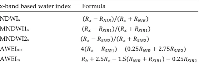
Table 3. Formulas of the x-band based water indexes for Landsat-8 OLI
x-band based water index Formula
NDWIx (𝑅𝑥− 𝑅𝑁𝐼𝑅)/(𝑅𝑥+ 𝑅𝑁𝐼𝑅)
MNDWI1x (𝑅𝑥− 𝑅𝑆𝐼𝑅1)/(𝑅𝑥+ 𝑅𝑆𝐼𝑅1)
MNDWI2x (𝑅𝑥− 𝑅𝑆𝐼𝑅2)/(𝑅𝑥+ 𝑅𝑆𝐼𝑅2)
AWEInsx 4(𝑅𝑥− 𝑅𝑆𝐼𝑅1) − (0.25𝑅𝑁𝐼𝑅+ 2.75𝑅𝑆𝐼𝑅2)
AWEIsx 𝑅𝑏+ 2.5𝑅𝑥− 1.5(𝑅𝑁𝐼𝑅+ 𝑅𝑆𝐼𝑅1) − 0.25𝑅𝑆𝐼𝑅2
x=ub: ultra-blue light, x=b: blue light, x=g: green light, x=r: red light
3.2. Image classification methods
3.2.1. Unsupervised image classification
The simplest unsupervised image classification method is to select a single threshold to
differentiate water and non-water pixels. Without computing any water index, a simple density slice method can be used to determine a threshold from the histogram of an image, i.e., choosing the digital
number associated with the valley of the histogram of the image as the threshold. Although this approach is simple to carry out, it is subject to uncertainty and errors if a histogram does not show a distinct valley. Using the computed water indexes for image classification, instead of selecting a
threshold based on the histogram, a zero-water index threshold method is usually chosen for extracting water features. This method can improve the efficiency of image classification, but it is also
subject to uncertainty and errors, because a threshold value of zero water index might not achieve the most accurate extraction of water body. Therefore, this study first evaluated the accuracy of the
extracted water features based on the zero-water index threshold method.
In addition to the simplest fixed single threshold method, a nonparametric and unsupervised
method for automatic threshold selection method proposed by Otsu (1979) was evaluated in this study. The principle of the Otsu’s method is to maximize the following objective function f:
𝑓 = 𝑃𝑊𝑃𝑁𝑊(𝜇𝑊− 𝜇𝑁𝑊)2 (6)
where PW and PNW are probabilities of water pixels and non-water pixels, respectively, W and NW
are mean water index values of classified water pixels and non-water pixels, respectively. The
optimal water index threshold is determined through searching the water index threshold (WIT) between -1 and 1 (as all the proposed water indexes are greater than zero for water pixels) with an
interval of 0.001 for maximizing the objective function shown in Eq.(6). All terms on the right hand of Eq.(6) are computed as follows:
𝑃𝑊=
𝑛𝑊
𝑛 , 𝑃𝑁𝑊=
𝑛𝑁𝑊
𝑛 , 𝜇𝑊=
∑𝑛𝑊𝑖=1𝑊𝐼𝑖
𝑛𝑊 , 𝜇𝑁𝑊=
∑𝑛𝑁𝑊𝑖=1 𝑊𝐼𝑖
𝑛𝑁𝑊 (7)
where WIi is water index of pixel i, n, nW, and nNW are numbers of total pixels, pixels with WI>WIT,
and pixels with WIWIT, respectively.
3.2.2. Supervised image classification
Given relative simplicity of identifying water or water-land boundary by human visual inspection, supervised classification might be a good choice for fulfilling the task of water pixel
neighbor, kNN (nearest neighbor), and etc. This study chose the KNN method to be evaluated because of its simplicity and effectiveness [45].
Applying the kNN method to determine if an unknown pixel x belongs to water class or non-water class, we first need to compute the spectral distance between the pixel x and each training pixel in m-dimensional spectral space as follows:
𝑑𝑖= ∑𝑚𝑗=1[(𝑅𝑥,𝑗− 𝑅𝑖,𝑗)2]1/2 (8)
where i is the index of training pixels, n is the number of training pixels, j is the band index, m is the
number of bands to be used in image classification, Rx,j is the spectral reflectance of the pixel x to be
classified in band j, and Ri,j is the spectral reflectance of the training pixel i in band j. All the computed
spectral distances between the unknown pixel x and all the training pixels will be ranked from the lowest to the highest. Based on k ranked spectral distances, the final step is to determine which class
the pixel x belongs to, and k is the number of the nearest training pixels to be considered in image classification. There are two questions must be answered before we can accomplish the final step: 1)
what is the suitable k value? and 2) what is the proper method for classifying unknown pixels? In this study, since we are interested in identifying water-body class, there are actually only two classes to be determined, i.e., water and non-water, and thus the training pixels either belong to water class
or non-water class. Therefore, we set k to be the number of training water pixels (nw).
With regard to the second question, two possible approaches can be used to solve this problem:
1) count the numbers of the nearest neighbors that belong to water class (kw) and non-water class (knw)
among the k ranked nearest training pixels (k=kw+knw). If kw is greater than knw, then the unknown
pixel belongs to water class, otherwise it belongs to non-water class. 2) compute the average spectral distance (dw) to the kw nearest water pixels and the average distance (dnw) to the knw nearest land
pixels. If dw is less than dnw, the unknown pixel belongs to water class, otherwise it belongs to
non-water class. However these two methods are subject to uncertainty associated with the selected k value, because a small variation in the selected k value could result in a different image classification
result. To eliminate such uncertainty, in this study we proposed to compute the sum of the inverse distances of each class among the identified k ranked nearest training pixels. For water-body
identification problem, there are only two classes, water or non-water, and thus we only need to compute two sums of the inverse distances. To avoid the division by zero (i.e., as the spectral distance
is zero), we first identify the minimum non-zero spectral distance (dmin) among the distances from
pixel x to all training pixels. If the computed spectral distance is zero, we set the inverse spectral
distance to be 2/dmin, otherwise the inverse spectral distance is 1/di, where di is the spectral distance
from pixel x to training pixel i. If the sum of the spectral distances to kw nearest water training pixels
greater than that to knw nearest non-water training pixels, pixel x is a water pixel, otherwise it is a
non-water pixel.
4. Results and Discussion
4.1. Benchmark data
Since no metadata file is available for each Google Earth image, we could not use pixel’s digital
number (DN) to compute the spectral reflectance without the required calibration parameters usually
in section 3.2.2 to extract water body. The only difference is that the digital number distance, rather than the spectral reflectance distance, is computed in the kNN classification.
For each Google Earth image, we first defined a rectangle covering a portion of water body and a portion of land. Then we carried out the kNN image classification inside the predefined rectangle. To reduce errors, the classification results need human visual inspection and correction, because
man-made structures, boats, and clouds could appear in the identified water body area. After the extraction of water body inside the predefined rectangle, the water-land boundary was identified for
defining a buffer zone with a width of 300 m (each side has a distance of 150 m to the water-land boundary). The buffer zones are the domains where the image classification results are evaluated. All
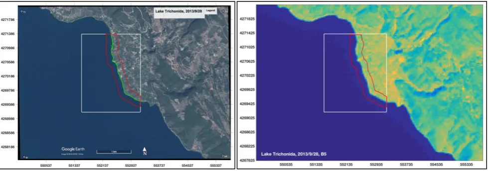
Google Earth images overlaid by the predefined polygon (in white) and the identified water-land boundary (in green) and the buffer zone (in red) are shown in the left column of Figure 2, and all the
corresponding Landsat-8 OLI band 5 images overlaid by the predefined polygon (in white) and the buffer zone (in red) are shown in the right column of Figure 2.
Figure 2. (left panel): 24 Google Earth images overlaid by the predefined polygon (in white) and the identified water-land boundary (in green) and the buffer zone (in red); (right panel): 24 Landsat-8 OLI band 5 images overlaid by the predefined polygon and the identified buffer zone
based on the corresponding Google Earth image.
4.2. Assessmenet of image classifcation results
In this study we employed a commonly used image classification accuracy index known as the Kappa coefficient () [45] to assess the image classification results among 24 selected lakes across the globe. The Kappa coefficient is defined as follows:
𝜅 =𝑝𝑟𝑜𝑏𝑎𝑏𝑖𝑙𝑖𝑡𝑦 𝑜𝑓 𝑐𝑜𝑟𝑟𝑒𝑐𝑡 𝑐𝑙𝑎𝑠𝑠𝑖𝑓𝑖𝑐𝑎𝑡𝑖𝑜𝑛−𝑝𝑟𝑜𝑏𝑎𝑏𝑖𝑙𝑖𝑡𝑦 𝑜𝑓 𝑐ℎ𝑎𝑛𝑐𝑒 𝑎𝑔𝑟𝑒𝑒𝑚𝑒𝑛𝑡
1−𝑝𝑟𝑜𝑏𝑎𝑏𝑖𝑙𝑖𝑡𝑦 𝑜𝑓 𝑐ℎ𝑎𝑛𝑐𝑒 𝑎𝑔𝑟𝑒𝑒𝑚𝑒𝑛𝑡 (9)
Corresponding to Eq.(9), the specific Kappa coefficient used in this study was computed as below:
𝜅 =(𝑃𝐿𝐺𝑤+𝑃𝐿𝐺𝑙)−(𝑃𝐿𝑤𝑃𝐺𝑤+𝑃𝐿𝑙𝑃𝐺𝑙)
1−(𝑃𝐿𝑤𝑃𝐺𝑤+𝑃𝐿𝑙𝑃𝐺𝑙) (10)
where PLGw is the probability that both Landsat and Google Earth place a pixel in water class, PLGl is the probability that both Landsat and Google Earth place a pixel in land class, PLw and PLl are the
probabilities that Landsat places a pixel in water class and land class, respectively, and PGw and PGl are the probabilities that Google Earth places a pixel in water class and land class, respectively. For
each selected lake, 60 combinations of 20 different water indexes (see Table 3) and three different image classification algorithms (i.e., the zero-water index threshold method, the Otsu method, and
the kNN method) were applied for extracting water body from Landsat imagery. The computed Kappa coefficients for three different image classification algorithms are listed in Tables 4-6 for the zero-water index threshold method, the Otsu method, and the kNN method, respectively. Based the
computed Kappa coefficient, the performance of an image classification method can be grouped into five categories[45]: poor (0.4), moderate (0.40.6), good (0.60.75), excellent (0.750.8), and
almost perfect (0.8). According to these criteria, all Kappa coefficients less than 0.76 (i.e., non-excellent) are labeled in red (see Tables 4-6). At each site, the highest Kappa coefficients among 20
different water indexes using a same image classification method are labeled in green (see Tables 4-6). For each image classification method, the average Kappa coefficient among 24 sites for each water
index is listed in the second last row of each table, and the associated mean rank (from high to low among 20 water indexes) is listed in the last row of each table (see Tables 4-6).
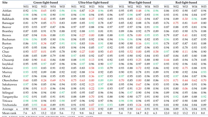
Table 4. Kappa coefficients of the Landsat-8 OLI classification results using the single threshold of zero water index method
WI1=NDWI, WI2=MNDWI, WI3=MNDWI2, WI4=AWEIns, WI5=AWEIs
0
Site Green-light-based Ultra-blue-light-based Blue-light-based Red-light-based
WI1 WI2 WI3 WI4 WI5 WI1 WI2 WI3 WI4 WI5 WI1 WI2 WI3 WI4 WI5 WI1 WI2 WI3 WI4 WI5
Atitlan 0.92 0.96 0.65 0.93 0.96 0.96 0.87 0.28 0.96 0.95 0.95 0.95 0.48 0.96 0.96 0.86 0.93 0.90 0.87 0.94 Baikal 0.98 0.96 0.98 0.90 0.98 0.94 0.98 0.94 0.95 0.96 0.97 0.98 0.97 0.93 0.98 0.93 0.91 0.94 0.84 0.97 Balkhash 0.94 0.89 0.42 0.95 0.89 0.89 0.80 0.17 0.92 0.85 0.91 0.85 0.22 0.94 0.87 0.94 0.89 0.30 0.96 0.89 Bansagar 0.81 0.79 0.85 0.73 0.83 0.89 0.85 0.92 0.78 0.87 0.85 0.82 0.88 0.76 0.85 0.76 0.75 0.81 0.69 0.80 Beaver 0.93 0.93 0.97 0.87 0.96 0.97 0.97 0.88 0.94 0.97 0.97 0.97 0.94 0.91 0.98 0.87 0.88 0.95 0.81 0.94 Brantley 0.87 0.85 0.91 0.78 0.88 0.92 0.88 0.93 0.81 0.91 0.89 0.86 0.92 0.79 0.89 0.86 0.83 0.90 0.76 0.88 Brown 0.87 0.94 0.06 0.88 0.95 0.94 0.27 0.00 0.88 0.88 0.95 0.76 0.00 0.95 0.95 0.79 0.87 0.41 0.81 0.92 Buchanan 0.96 0.96 0.95 0.90 0.96 0.94 0.95 0.92 0.94 0.94 0.96 0.96 0.94 0.92 0.95 0.96 0.95 0.94 0.87 0.95 Burton 0.86 0.91 0.34 0.87 0.91 0.91 0.83 0.06 0.91 0.90 0.90 0.90 0.16 0.91 0.91 0.78 0.87 0.87 0.81 0.88 Caspian 0.95 0.95 0.84 0.96 0.93 0.94 0.94 0.85 0.97 0.92 0.95 0.95 0.87 0.96 0.93 0.94 0.95 0.78 0.93 0.93 Chao 0.93 0.57 0.01 0.95 0.78 0.90 0.27 0.00 0.93 0.45 0.93 0.52 0.00 0.95 0.58 0.97 0.90 0.11 0.96 0.90 Chelan 0.88 0.85 0.89 0.79 0.90 0.97 0.93 0.92 0.87 0.95 0.95 0.90 0.92 0.84 0.93 0.87 0.84 0.85 0.80 0.88 Chuzenji 0.80 0.90 0.41 0.84 0.88 0.88 0.95 0.13 0.91 0.92 0.85 0.93 0.25 0.88 0.90 0.44 0.85 0.94 0.78 0.85 Issykkul 0.95 0.95 0.97 0.87 0.96 0.96 0.97 0.96 0.90 0.97 0.96 0.96 0.97 0.89 0.97 0.93 0.92 0.96 0.82 0.96 Mohave 0.93 0.93 0.83 0.91 0.92 0.85 0.83 0.58 0.93 0.79 0.93 0.88 0.72 0.92 0.86 0.92 0.92 0.75 0.88 0.91 Murray 0.93 0.92 0.89 0.88 0.92 0.82 0.88 0.54 0.92 0.85 0.90 0.91 0.78 0.91 0.89 0.91 0.90 0.92 0.84 0.93 Ohrid 0.97 0.96 0.84 0.95 0.95 0.95 0.93 0.36 0.97 0.93 0.97 0.95 0.83 0.96 0.95 0.92 0.97 0.84 0.87 0.96 Okeechobee 0.60 0.85 0.24 0.69 0.74 0.75 0.63 0.00 0.89 0.89 0.70 0.85 0.00 0.80 0.86 0.51 0.71 0.44 0.62 0.70
Table 5. Kappa coefficients of the Landsat-8 OLI classification results using the Otsu method
1
WI1=NDWI, WI2=MNDWI, WI3=MNDWI2, WI4=AWEIns, WI5=AWEIs
2
Site Green-light-based Ultra-blue-light-based Blue-light-based Red-light-based
WI1 WI2 WI3 WI4 WI5 WI1 WI2 WI3 WI4 WI5 WI1 WI2 WI3 WI4 WI5 WI1 WI2 WI3 WI4 WI5
Atitlan 0.91 0.91 0.93 0.94 0.94 0.94 0.94 0.95 0.94 0.95 0.93 0.93 0.95 0.94 0.95 0.89 0.88 0.89 0.94 0.93 Baikal 0.94 0.90 0.90 0.97 0.96 0.95 0.93 0.93 0.97 0.97 0.94 0.92 0.92 0.97 0.97 0.91 0.86 0.85 0.97 0.96 Balkhash 0.93 0.96 0.95 0.91 0.96 0.94 0.96 0.93 0.89 0.95 0.94 0.96 0.94 0.91 0.96 0.92 0.95 0.96 0.89 0.95 Bansagar 0.77 0.74 0.74 0.82 0.83 0.78 0.75 0.76 0.82 0.83 0.77 0.75 0.75 0.82 0.83 0.77 0.71 0.71 0.83 0.84 Beaver 0.90 0.87 0.88 0.96 0.96 0.92 0.91 0.92 0.97 0.97 0.91 0.90 0.90 0.97 0.97 0.87 0.83 0.83 0.97 0.96 Brantley 0.79 0.78 0.79 0.93 0.93 0.81 0.80 0.82 0.94 0.94 0.80 0.79 0.80 0.94 0.94 0.78 0.75 0.77 0.93 0.93 Brown 0.89 0.85 0.86 0.95 0.95 0.93 0.90 0.90 0.95 0.95 0.92 0.89 0.89 0.95 0.95 0.88 0.83 0.84 0.95 0.94 Buchanan 0.93 0.93 0.93 0.93 0.93 0.94 0.94 0.94 0.93 0.93 0.94 0.93 0.93 0.93 0.93 0.93 0.92 0.92 0.91 0.91 Burton 0.85 0.86 0.87 0.91 0.91 0.88 0.89 0.90 0.91 0.91 0.87 0.88 0.89 0.91 0.91 0.82 0.82 0.83 0.91 0.91 Caspian 0.95 0.96 0.94 0.90 0.90 0.96 0.97 0.96 0.92 0.92 0.96 0.97 0.96 0.91 0.92 0.93 0.95 0.90 0.89 0.87 Chao 0.91 0.94 0.95 0.93 0.88 0.92 0.95 0.95 0.93 0.88 0.91 0.95 0.95 0.93 0.88 0.89 0.94 0.94 0.92 0.91 Chelan 0.83 0.79 0.80 0.92 0.95 0.88 0.85 0.86 0.93 0.96 0.86 0.83 0.84 0.93 0.96 0.84 0.81 0.82 0.91 0.92 Chuzenji 0.87 0.85 0.86 0.94 0.89 0.88 0.88 0.88 0.93 0.92 0.87 0.87 0.88 0.93 0.91 0.77 0.85 0.85 0.94 0.84 Issykkul 0.89 0.86 0.86 0.97 0.96 0.90 0.88 0.88 0.97 0.97 0.90 0.88 0.88 0.97 0.97 0.90 0.83 0.82 0.97 0.93 Mohave 0.90 0.89 0.90 0.86 0.88 0.91 0.91 0.91 0.86 0.88 0.90 0.90 0.91 0.87 0.88 0.88 0.86 0.86 0.86 0.89 Murray 0.89 0.88 0.90 0.90 0.92 0.90 0.90 0.91 0.89 0.91 0.90 0.89 0.91 0.89 0.91 0.85 0.83 0.86 0.89 0.91 Ohrid 0.97 0.94 0.92 0.96 0.90 0.97 0.95 0.94 0.97 0.93 0.97 0.94 0.93 0.97 0.93 0.90 0.91 0.88 0.95 0.87 Okeechobee 0.58 0.64 0.69 0.87 0.75 0.65 0.70 0.75 0.86 0.75 0.61 0.69 0.72 0.83 0.75 0.55 0.60 0.64 0.83 0.74
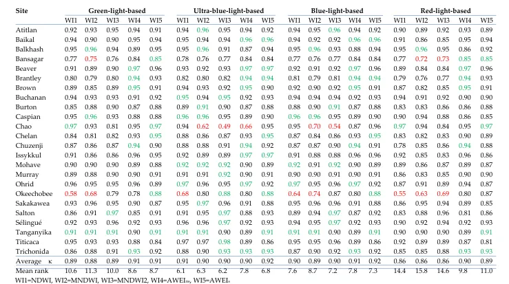
Table 6. Kappa coefficients of the Landsat-8 OLI classification results using the KNN method
3
WI1=NDWI, WI2=MNDWI, WI3=MNDWI2, WI4=AWEIns, WI5=AWEIs
4
Site Green-light-based Ultra-blue-light-based Blue-light-based Red-light-based
WI1 WI2 WI3 WI4 WI5 WI1 WI2 WI3 WI4 WI5 WI1 WI2 WI3 WI4 WI5 WI1 WI2 WI3 WI4 WI5
Based on the image classification results using the zero-water index threshold method listed in
Table 4, we can find that the modified normalized water index (i.e., MNDWI2) using the shortwave infrared band 2 (i.e., SIR2) performed poorly in extracting water features, no matter green light, ultra-
blue light, or blue light are used, because the average Kappa coefficients of MNDWI2g, MNDWI2ub,
and MNDWI2b are all less than 0.76. For the red-light band based MNDWI2r, the average Kappa
coefficient is just at 0.76. Those results indicate that using the zero-water index threshold method for extracting water features from Landsat imagery, the SIR2-based MNDWI2 should not be used as the water index. Among 20 water indexes, only two water indexes, i.e., AWEInsub and AWEInsb, produced
the Kappa coefficients that are all greater than 0.75 (i.e., excellent). According to Table 4, among 24 sites, AWEInsub achieved eight highest Kappa coefficients while AWEInsb only produced three highest
Kappa coefficients.
Comparing the computed Kappa coefficients of the image classification results using the Otsu
method listed in Table 5 to the Kappa coefficients using the zero-water index threshold method listed in Table 4, we can find that the Otsu method produced better results than the zero-water index
threshold method, because overall there are only 24 Kappa coefficients less than 0.76 for the Otsu method, while the zero-water index threshold method produced 60 Kappa coefficients less than 0.76 which is more than double of the number for the Otsu method. On the other hand, all the average
Kappa coefficients listed in Table 5 are greater than 0.75. The automatic selection of water index threshold value in the Otsu method determines that the Otsu method is better than just using a
threshold water index value of zero to differentiate water and non-water pixels. Among 20 different water indexes, AWEIns performed better than other types of water indexes, no matter it is ultra-blue
light, blue light, green light or red light based AWEIns, because they all produced greater than 0.75
Kappa coefficients at 24 sites, as the Otsu method is used for image classification. Among 4 types of
AWEIns, the ultra-blue light based AWEInsub is the best.
According to Table 6, as one type of supervised image classification method, the kNN algorithm only resulted in 16 Kappa coefficients that are below 0.76, and 99.2% image classification results are
excellent or almost perfect. The number of non-excellent image classification results produced by the kNN method dropped about 33% compared to the Otsu method. The improvement in the extracted
water features by the kNN method implies that with human intervenes the classification results can be improved. However, the improvement in the image classification by the kNN method is associated
with high computational cost as the computational time for the kNN method is much longer than unsupervised methods, such as the single threshold method and the Otsu method.
Among the 24 tested lakes, the selected area of Okeechobee lake caused troubles for most of water indexes of NDWIs and MNDWIs, and only AWEIns worked well for extracting water body in
this area, no matter which visible light band is used in the AWEIns. The complex pattern of the
shoreline in the selected area of Okeechobee lake as shown in Figure 2 is the potential cause of the poor performance of image classification by NDWIs and MNDWIs.
5. Conclusions
This paper addressed three important issues related to extraction of water features from Landsat
imagery: How to collect ground truth data across the globe for validating Landsat image classification results? Which water indexes (among NDWI, MNDWI, AWEI) and which image classification
First, this study took advantage of high resolution satellite images archived in Google Earth to obtain 24 high resolution ( 5 m) and cloud-free images and each image covers a portion of 24 selected lakes
across the globe. Corresponding to these high resolution Google Earth images, 24 Landsat-8 OLI cloud-free images covering the same areas with the same (or 1 day) acquisition dates of the Google Earth images were downloaded from the USGS Earth Explorer website. Each Landsat image was
clipped to the same spatial extent and resampled to the same grid cell size of the corresponding Google Earth image using clip and resample raster functions of the ArcMap. Each Google Earth
imagery georeferencing was corrected by the following two steps: 1) use the ArcMap’s raster shift
function to shift the Google Earth image with the visual inspection detected x and y shift values
through comparing the Google Earth image and the corresponding Landsat-8 OLI band 8 image, and 2) compute the spatial correlation coefficients between the Google Earth image and the Landsat-8
OLI band 8 image with different shift values in the x and y directions of the Google Earth image, choose the x and y shift values associated with the maximum correlation coefficient as the optimal x
and y shift values, and correct the georeferencing of the Google Earth image using the optimal x and y shift values.
To generate the benchmark data for evaluating the Landsat image classification results, a
polygon was first defined to cover a portion of each selected lake area. The kNN method was then applied to each Google Earth image for carrying out image classification inside the predefined
polygon. Since no metadata are available for the Google Earth images, no water indexes can be computed and thus digital numbers in three channels (RGB) were utilized for image classification.
The extracted water body from each Google Earth image was also verified and manually corrected by visual inspection. For a fair comparison among 24 selected lakes, a buffer zone with the central line along the detected water-land boundary and a width (perpendicular to the central line) of 300 m
was constructed for each Google Earth image. This constructed buffer zone was then used as the comparison domain for assessing the Landsat image classification results.
With regard to the computed water index for identifying water pixels from Landsat imagery, in addition to the commonly used green light based water indexes, Landsat-8 OLI’s ultra-blue, blue, and red light band based water indexes were also tested in this research. The rationale behind this is that clear water has higher spectral reflectance in the blue light band than the green and red light
bands. For turbid water especially with high concentration of sediment loads, its spectral reflectance in the red light band might be higher than in the blue or green light bands [38-40]. Therefore, this
study tested four sets of water indexes corresponding to four visible light (ultra-blue, blue, green, and red) bands of Landsat-8 OLI. Each set of water indexes contain: 1) normalized difference water index (i.e., NDWI), 2) modified normalized difference water index using the first shortwave infrared
(SIR1) band (MNDWI), 3) modified normalized difference water index using the second shortwave infrared (SIR2) band (MNDWI2), 4) automated water extraction index without shadow (AWEIns), and
5) automated water extraction index with shadow (AWEIs). With regard to the image classification,
two unsupervised methods i.e., the single zero-water index threshold method, and the Otsu’s
automatic threshold selection method, and the supervised kNN method were employed for conducting the image classification. Overall, 60 combined methods (20 water indexes 3 image
from the high resolution Google Earth images. The following conclusions have been drawn based on the computed Kappa coefficients.
The kNN method is better than the Otsu method, and the Otsu method is better than the single zero-water index threshold method. But the computational efficiency associated with the kNN method is very low compared with other two methods. Therefore, if the computational cost is not an
issue, the kNN method combined with the AWEInsub (i.e., the ultra-blue light based AWEIns) is the
best method for extracting water features from Landsat imagery because of its top one average rank
in terms of the Kappa coefficients (see Table 6). If the computational cost is taken into account, the Otsu method is a good choice.
AWEIns and AWEIs are better than NDWI, MNDWI and MNDWI2. If the single zero-water index
threshold method is used for image classification, MNDWI2 should be avoided because of its poor
performance in differentiating water and non-water pixels. AWEIns works better than AWEIs under
the Otsu method, and the average rank of the image classification accuracy from high to low is the
ultra-blue light, blue light, green light, and red light based AWEIns. This finding actually proved that
a blue light band in water index might be better than a green light band for clear water because the spectral reflectance of clear water usually is higher in blue light than any other visible light bands.
On the other hand, if lake water is turbid or sediment-laden, the red-light band based water indexes might work better than other visible light bands in detecting water body because turbid or
sediment-laden water reflects red light stronger than other visible light [38]. However, none of the red light based water indexes showed any improvement in extracting water features in this study, which is
probably due to the fact that none of the 24 selected lakes had high sediments loads leading to high reflectance in red light.
Author Contributions: F.P. conceived and designed the study; F.P., X.X., and C.W. processed and analyzed Google Earth and Landsat-8 OLI images. F.P. wrote the paper.
Funding: This study was funded in part by the Joint Research Fund for Overseas Chinese Scholars and Scholars in Hong Kong and Macao of National Natural Science Foundation of China (No. 41628101) and General Program of National Natural Science Foundation of China (No. 41871264).
References
1. Allen, G.H.; Pavelsky, T.M. Global extent of rivers and streams. Science 2018, 361, 585-588.
2. Shiklomanov, I.A.; Sokolov, A.A. Methodological basis of water balance investigation and computation. In New Approaches in Water Balance Computations. International Association for Hydrological Sciences Publ. No.148. 1983.
3. Dingman, S.L. Physical Hydrology, 3rd ed.; Waveland Press, INC.: Long Grove, Illinois, USA, 2015; p.643. 4. Hornberger, G.M.; Wiberg, P.L.; Raffensperger, J.P.; D’Odorico, P. Elements of Physical Hydrology, 2nd ed.;
Johns Hopkins University Press: Baltimore, USA, 2014; p.378.
5. Overton, I.C. Modeling floodplain inundation on a regulated river: integrating GIS, remote sensing and hydrological models. River Research and Applications 2005, 21, 91-101.
6. Matgen, P.; Schumann, G.; Henry, J.P.; Hoffmann, L.; Pfister, L. Integration of SAR derived river inundation areas, high-precision topographic data and a river flow model toward near real-time flood management. International Journal of Applied Earth Observation and Geoinformation 2007, 9(3), 247-263.
8. Ban, H.; Kwon, Y.; Shin, H.; Ryu, H.; Hong, S. Flood monitoring using satellite based RGB composite imagery and refractive index retrieval visible and near-infrared bands. Remote Sensing2017, 9, 313, doi: 10.3390/rs9040313.
9. Pelletier, J.D.; Mayer, L.; Pearthree, P.A.; House, P.K.; Demsey, K.A.; Klawon, J.E.; Vincnet, K.R. An integrated approach to flood hazard assessment on alluvial fans using numerical modeling, field mapping, and remote sensing. Geological Society of America Bulletin 2005, 117, 1167-1180.
10. Sanyal, J.; Lu, X. Remote sensing and GIS-based flood vulnerability assessment of human settlements: a case study of Gangetic West Bengal, India. Hydrological Processes 2005, 19, 3699-3716.
11. Sakamoto, T.; Van Nguyen, N.; Kotear, A.; Ohno, H.; Ishitsuka, N.; Yokozawa, M. Detecting temporal changes in the extent of annual flooding within the Cambodia and the Vietnamese Mekong Delta from MODIS time-series imagery. Remote Sensing of Environment 2007, 109, 295-313.
12. Taubenbock, H.; Wurm, M.; Netzband, M.; Zwenzner, H.; Roth, A.; Rahman, A.; Dech, S. Flood risks in urbanized areas-multi-sensoral approaches using remotely sensed data for risk assessment. Natural Hazards and Earth System Sciences 2011, 11, 431-444.
13. Skakun, S.; Kussul, N.; Shelestov, A.; Kussui, O. Flood hazard and flood risk assessment using a time series of satellite images: a case study in Namibia. Risk Analysis 2014, 34, 1521-1537.
14. Rahman, M.S.; Di, L. The state of the art of spaceborne remote sensing in flood management. Natural Hazards 2017, 85, 1223-1248.
15. Rosser, J.F.; Leibovici, D.G.; Jackson, M.J. Rapid flood inundation mapping using social media, remote sensing an topographic data. Natural Hazards 2017, 87, 103-120.
16. Huang, X.; Wang, C,; Li, Z. Reconstructing flood inundation probability by enhancing near real-time imagery with real-time gauges and tweets. IEEE Transactions on Geoscience and Remote Sensing 2018, 56(8), 4691-4701.
17. Psomiadis, E.E.; Soulis, K.X.; Zoka, M.; Decas, N. Synergistic approach of remote sensing and GIS techniques for flash-flood monitoring and damage assessment in Thessaly Plain Area, Greece. Water 2019, 11, doi:10.3390/w11030448.
18. Frappart, F.; Papa, F.; Famiglietti, J.S.; Prigent, C.; Rossow, W.B.; Seyler, F. Interannual variations of river water storage from a multiple satellite approach: A case study for the Rio Negro River basin. Journal of Geophysical Research-Atmospheres 2008, 113 (D21), D21104.
19. Cai, X.; Gan, W.; Ji, W. Zhao, Z.; Wang, X.; Chen, X. Optimizing remote sensing-based level-area modeling of large lake wetlands: case study of Poyang Lake. IEEE Journal of Selected Topics in Applied Earth Observations and Remote Sensing 2015, 8(2), 471-479.
20. Normandin, C.; Frappart, F.; Lubac, B.; Belanger, S. Marieu, V.; Blarel, F.; Robinet, A.; Guiastrennec-Faugas, L. Quantification of surface water volume changes in the Mackenzie Delta using satellite multi-mission data. Hydrology and Earth System Sciences 2018, 22(2), 1543-01561.
21. Schwerdtfeger, J.; da Silveira, S.W.; Zeilhofer, P.; Weiler, M. Coupled ground- and space- based assessment of regional inundation dynamics to asses impact of local and upstream changes on evaporation in tropical wetlands. Remote Sensing 2015, 7, 9769-9795.
22. Pan, F.; Nichols, J. Remote sensing of river stage using the cross sectional inundation area-river stage relationship (IARSR) constructed from digital elevation model data. Hydrological Processes 2012, 27, 3596-3606.
23. Pan, F. Remote sensing of river stage and discharge. SPIE Newsroom 2013, doi:10.1117/2.1201212.0461. http://spie.org/x91480.xml?pf=true&ArticleID=x91480
24. Pan, F.; Liao, J.; Li, X.; Guo, H. Application of the inundation area-lake level rating curves constructed from the SRTM DEM to retrieving lake levels from satellite measured inundation areas. Computers and Geosciences 2013, 52, 168-176.
25. Pan, F.; Wang, C.; Xi, X. Constructing river stage-discharge rating curves using remotely sensed river cross-sectional inundation areas and river bathymetry. Journal of Hydrology 2016, 540, 670-687.
26. Ridolfi, E.; Di Francesco, S.; Pandolfo, C.; Berni, N. Biscarini, C.; Manciola, P. Coping with extreme events: effect of different reservoir operation strategies on flood inundation maps. Water 2019, 11, doi:10.3390/w11050982.
28. Dadson, S.J.; Ashpole, I.; Harris, P.; Davies, H.N.; Clark, D.B.; Blyth, E.; Taylor, C.M. Wetland inundation dyanmics in a model of land surface climate: Evaluation in the Niger inland delta region. Journal of Geophysical Research – Atmospheres 2010, 115, D23114.
29. Prigent, C.; Papa, F.; Aires, F.; Rossow, W.B.; Matthews, E.E. Global inundation dynamics inferred from multiple satellite observations. Journal of Geophysical Research – Atmospheres 2007, 112, D12107.
30. Sheffield, J.; Ferguson, C.R.; Troy, T.J. Wood, E.F.; McCabe, M.F. Closing the terrestrial water budget from satellite remote sensing. Geophysical Research Letters 2009, 36, L07403.
31. Shi, L.; Ling, F.; Foody, G.M.; Chen, C.; Fang, S.; Li, X.; Zhang, Y.; Du, Y. Permanent disappearance and seasonal fluctuation of urban lake area in Wuhan, China monitored with long time series remotely sensed images from 1987 to 2016. International Journal of Remote Sensing 2019, 40, 8484-8505.
32. Li, W.; Du Z.; Ling, F.; Zhou, D.; Wang, H.; Gui, Y.; Sun, B.; Zhang, X. A comparison of land surface water mapping using the normalized difference water index from TM, ETM+ and ALI. Remote Sensing 2013, 5, 5530-5549, doi:10.3390/rs5115530.
33. Ronki, K.; Ahmad, A.; Selamat, A.; Hazini, S. Water feature extraction and change detection using multitemporal Landsat imagery. Remote Sensing 2014, 6, 4173-4189, doi:10.3390/rs6054173.
34. Yang, Y.; Liu, Y.; Zhou M.; Zhang, S.; Zhan, W.; Sun, C. Landsat 8 OLI image based terrestrial water extraction from heterogeneous backgrounds using a reflectance homogenization approach. Remote Sensing of Environment 2015 ,171, 14-32.
35. Zhou, Y.; Dong, J.; Xiao, X.; Xiao, T.; Yang, Z.; Zhao, G.; Zou, Z.; Qin, Y. Open surface water mapping algorithms A comparison of water-related spectral indices and sensors. Water 2017, 9, 256, doi:10.3390/w9040256.
36. Bangira, T.; Alfieri, S.M.; Menenti, M.; van Niekerk, A. Comparing thresholding with machine learning classifiers for mapping complex water. Remote Sensing 2019, 11, 1351, doi:10.3390/rs11111351.
37. Schwatke, C.; Scherer, D.; Dettmering, D. Automated extraction of consistent time-variable water surfaces of lakes and reservoirs based Landsat and Sentinel-2. Remote Sensing 2019, 11, 1010, doi:10.3390/rs11091010. 38. Bartolucci, L.A.; Robinson, B.F.; Silva, L.F. Field measurements of the spectral response of natural waters.
Photogrammetric Engineering and Remote Sensing 1977, 43, 595-598.
39. Meaden, G.J.; Kapetsky, J.M. Geographical information system and remote sensing in inland fisheries and aquaculture. FAO Fisheries Technical Paper No.318 1991, Rome, FAO, p.261.
40. Jensen, J.R. Introductory Digital Image Processing: A Remote Sensing Perspective, 2nd ed.; Upper Saddle River, New Jersey, USA, Prentice-Hall 1995.
41. McFeeters, S.K. The use of the normalized difference water index (NDWI) in the delineation of open water features. International Journal of Remote Sensing 1996, 17, 1425-1432.
42. Xu, H. Modification of normalized difference water index (NDWI) to enhance open water features in remotely sensed imagery. International Journal of Remote Sensing 2006, 27, 3025-3033.
43. Feyisa, G.L.; Meilby, H.; Fensholt, R.; Proud, S.R. Automated water extraction index: A new technique for surface water mapping using Landsat imagery. Remote Sensing of Environment 2014, 140, 23-35.
44. Otsu, N. A threshold selection method from gray-level histograms. IEEE Transactions on Systems, Man, Cybernetics 1979, 9, 62-69.