This work is protected by copyright and other intellectual property rights and
duplication or sale of all or part is not permitted, except that material may be
duplicated by you for research, private study, criticism/review or educational
purposes. Electronic or print copies are for your own personal,
non-commercial use and shall not be passed to any other individual. No quotation
may be published without proper acknowledgement. For any other use, or to
quote extensively from the work, permission must be obtained from the
Statistical analysis of longitudinal
randomized clinical trials with missing
data: a comparison of approaches
Royes Joseph
A thesis submitted for the degree of Doctor of Philosophy
March 2015
Research Institute for Primary Care and Health Sciences
Declaration Part 1
Declaration
SUBMISSION OF THESIS FOR A RESEARCH DEGREE
Degree for which thesis being submitted: PhD
Title of thesis: Statistical analysis of longitudinal randomized clinical trials with missing data: a comparison of approaches
This thesis contains confidential information and is subject to the protocol set down for the submission and examination of such a thesis. No
Date of submission: 05 November 2014 Original registration date: 01 October 2011
Name of candidate: Royes Joseph
Research Institute: Primary Care and Health Sciences Name of Lead Supervisor: Dr Martyn Lewis
I certify that:
(a) The thesis being submitted for examination is my own account of my own research
(b) My research has been conducted ethically. Where relevant a letter from the approving body confirming that ethical approval has been given has been bound in the thesis as an Annex
(c) The data and results presented are the genuine data and results actually obtained by me during the conduct of the research
(d) Where I have drawn on the work, ideas and results of others this has been appropriately acknowledged in the thesis
(e) Where any collaboration has taken place with one or more other researchers, I have included within an ‘Acknowledgments’ section in the thesis a clear
statement of their contributions, in line with the relevant statement in the Code of Practice (see Note overleaf).
(f) The greater portion of the work described in the thesis has been undertaken subsequent to my registration for the higher degree for which I am submitting for examination
(g) Where part of the work described in the thesis has previously been incorporated in another thesis submitted by me for a higher degree (if any), this has been identified and acknowledged in the thesis
(h) The thesis submitted is within the required word limit as specified in the Regulations
Total words in submitted thesis (including text and footnotes, but excluding references and appendices): 64624
Abstract
Objectives
Missing data represent a source of bias in randomized clinical trials (RCTs). This thesis focuses on pragmatic RCTs with missing continuous outcome data and evaluates the use and appropriateness of current methods of analysis.
Methods
This thesis consists of three parts. First, a systematic review examined practices relating to missing data in published RCTs. Second, a simulation study compared the performance of various methods for handling missing data in a number of plausible trial scenarios. Finally, an empirical evaluation of two pragmatic RCTs investigated the use of a reminder process to inform whether missingness is likely to be non-ignorable.
Results
The majority of 91 trials in the systematic review adopted a form of single imputation, such as last observation carried forward (LOCF) for dealing with missing data. Mixed-effects model for repeated measures (MMRM) and/or multiple imputation (MI) were limited to eight trials. Sensitivity analyses were infrequently and inappropriately used, and insufficiently reported.
In the simulation study, LOCF yielded biased estimates of treatment effect in most scenarios, irrespective of missing data mechanisms. All methods, except LOCF, yielded unbiased estimates for scenarios of equal dropout rate and same direction of dropout in both treatment groups. MMRM and MI were more robust to bias than complete-case and LOCF-based analyses.
In the empirical study, the evaluation using reminder responses indicated the possibility of biased MMRM estimation in one trial and unbiased MMRM estimation in the other.
Conclusion
CCA and LOCF-based analysis should be disregarded in favour of methods such as MMRM and MI-based analysis. The proposed reminder approach can be used to assess the robustness of the missing at random (MAR) assumption by checking expected consistency in MAR-based estimates. If the results deviate, then analyses incorporating a range of plausible missing not at random assumptions are advisable, at least as sensitivity tests for the evaluation of treatment effect.
Table of contents
Declaration ... i
Abstract ... ii
Table of contents ... iv
List of tables ... xi
List of figures ... xiii
List of abbreviations ... xvi
List of publications ... xviii
Acknowledgements ... xix
Chapter 1: Introduction ... 1
1.1 The present study: research issues ... 1
1.2 Outline of thesis ... 3
Chapter 2: Background ... 6
2.1 Introduction ... 6
2.2 The problem of missing data in clinical trials ... 6
2.3 Missing data: theoretical framework ... 11
2.3.1 Missing data patterns... 12
2.3.2 Missing data mechanism ... 13
2.3.3 Identification of the missing data mechanism ... 15
2.4 Methods for handling incomplete continuous data ... 15
2.4.1 Description of candidate approaches to analysing longitudinal RCT data with missing values ... 16
2.4.2 Choice of approach to handling missing data: existing literature on
comparisons of the approaches ... 27
2.4.3 Sample size calculation in anticipation of dropouts ... 34
2.5 Guidance on prevention and handling of missing data in RCTs ... 35
2.6 Rationale of the thesis ... 36
2.7 Conclusion ... 38
Chapter 3: Systematic review ... 40
3.1 Introduction ... 40
3.2 Background ... 40
3.2.1 RCTs in MSCs ... 44
3.2.2 ITT analysis and missing outcome data in trials in MSCs ... 45
3.2.3 Handling of missing outcome data in trials in MSCs ... 46
3.3 Objectives ... 46
3.4 Methods ... 47
3.4.1 Selection of studies ... 47
3.4.2 Data extraction and management ... 50
3.5 Results ... 55
3.5.1 Characteristics of included trials ... 55
3.5.2 Dropouts ... 57
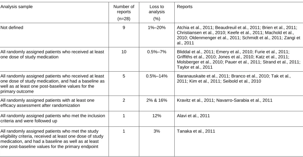
3.5.3 Analysis strategy and loss to analysis ... 60
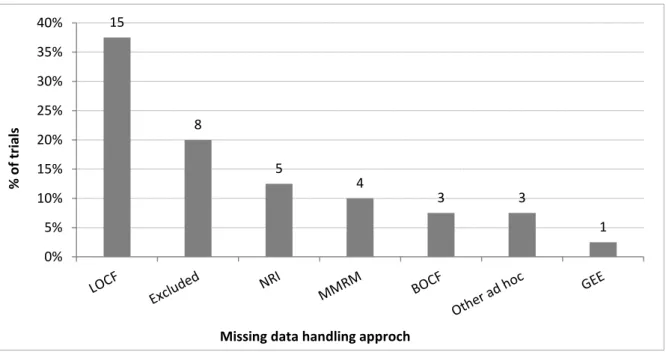
3.5.4 Handling of dropouts: imputation strategy ... 63
3.5.5 Sensitivity analysis and cautionary notes on missing data ... 65
3.6.1 Overall summary ... 67
3.6.2 Quality of reporting ... 68
3.6.3 Importance of collecting data on all randomized subjects ... 69
3.6.4 Power calculation in anticipation of dropouts ... 70
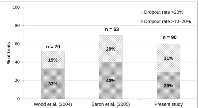
3.6.5 Dropout rate ... 71
3.6.6 Analysis strategy ... 74
3.6.7 Baseline comparison ... 76
3.6.8 Handling missing data ... 77
3.6.9 Sensitivity analysis ... 81
3.7 Limitations and generalizability ... 82
3.8 Conclusion ... 82
Chapter 4: Simulation study: an overview of design ... 84
4.1 Introduction ... 84
4.2 Background ... 85
4.3 Simulation procedure ... 86
4.3.1 Step 1: Generating complete datasets ... 86
4.3.2 Step 2: Generating missing data ... 93
4.3.3 Step 3: Imputation and analysis methods ... 97
4.4 Measures of performance ... 99
4.4.1 Bias ... 99
4.4.2 Overall accuracy of the estimate ... 100
4.4.4 Average width of confidence interval ... 101
4.4.5 Statistical power ... 101
4.5 Summary of simulation scenarios ... 102
4.6 Discussion and conclusion ... 104
Chapter 5: Simulation study - findings 1 ... 109
5.1 Introduction ... 109
5.2 Bias and precision ... 112
5.2.1 Bias and RMSE under MCAR ... 112
5.2.2 Bias and RMSE under MAR dependent on baseline value (MAR-B)... 116
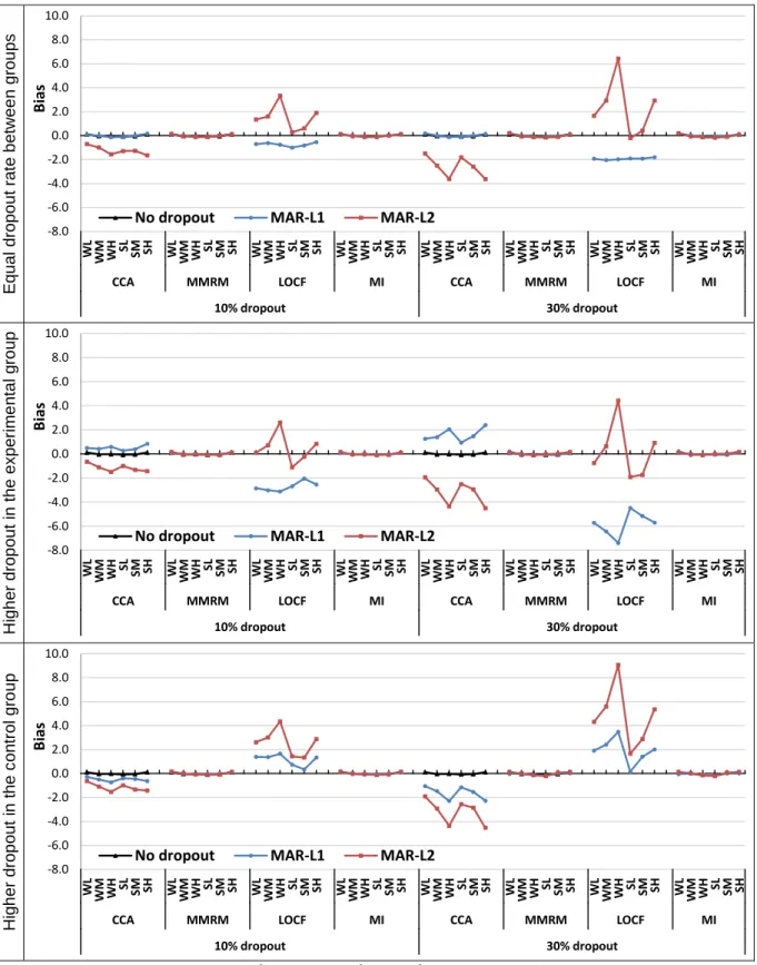
5.2.3 Bias and RMSE under MAR dependent on last observed value (MAR-L) .... 119
5.2.4 Bias and RMSE under MNAR ... 123
5.3 Confidence interval coverage and width... 127
5.3.1 CI coverage and width under MCAR ... 128
5.3.2 CI coverage and width under MAR-B ... 131
5.3.3 CI coverage and width under MAR-L ... 134
5.3.4 CI coverage and width under MNAR ... 138
5.4 Statistical power to detect the true difference ... 141
5.4.1 Statistical power under MCAR ... 142
5.4.2 Statistical power under MAR-B ... 144
5.4.3 Statistical power under MAR-L ... 146
5.4.4 Statistical power under MNAR ... 148
Chapter 6: Simulation study: findings 2... 152
6.1 Introduction ... 152
6.2 Effect of trajectory pattern and size of treatment effect on inferences from the missing data handling approaches ... 153
6.3 Comparison of two strategies for handling baseline data in an MMRM analysis... ... 159
6.3.1 Effects on overall accuracy ... 160
6.3.2 Effects on the coverage of 95% CI ... 160
6.3.3 Effects on the observed power ... 163
6.4 Effect of sample size on power under different missing data mechanisms: a comparison of missing data handling approaches ... 165
6.4.1 When the desired power was 90% in the absence of missing data ... 166
6.4.2 When the desired power was 80% in the absence of missing data ... 171
6.5 Summary of findings ... 174
6.6 Overall summary of findings from simulation studies... 176
Chapter 7: An empirical evaluation of the impact of missing data on treatment effect: analysis of TATE and STarT Back trials ... 178
7.1 Introduction ... 178
7.2 Background ... 178
7.3 Reminder responses as proxies of non-responses ... 179
7.4 Methods ... 181
7.5 The TATE trial... 184
7.5.2 Analysis of the incomplete TATE trial – estimation of treatment effect at month
12 ... 193
7.5.3 Summary and interpretation of findings ... 198
7.6 The STarT Back trial ... 201
7.6.1 Descriptive analysis of missing data ... 202
7.6.2 Analysis of STarT Back trial data – estimation of the treatment effect at month 12 ... 209
7.6.3 Summary and interpretation of findings ... 213
7.7 Discussion ... 214
7.8 Conclusion ... 219
Chapter 8: Summary, discussion and conclusions ... 221
8.1 Introduction ... 221
8.2 Summary of findings ... 222
8.2.1 Summary of systematic review ... 222
8.2.2 Summary of simulation study ... 224
8.2.3 Summary of empirical evaluation ... 228
8.3 Discussion of the findings ... 230
8.3.1 The performance of incomplete data analysis methods for the estimation of treatment effect in RCTs ... 230
8.3.2 Choice between MMRM and MI-based analyses in an RCT ... 237
8.3.3 Strategy for handling baseline values with MMRM analysis ... 241
8.3.4 The benefits of sample size inflation to the effect of attrition on statistical power ... 242
8.4 Limitations and generalizability ... 248
8.5 Implications for practice ... 250
8.6 Future work ... 253
8.7 Conclusion ... 254
References ... 256
List of tables
Table 2.1: Percent efficiency of MI estimation ... 22
Table 3.1: Classification of analysis strategy used in trial reports ... 53
Table 3.2: Description of the selected trials (n=91) ... 56
Table 3.3: Size of the trial ... 57
Table 3.4: Analysis strategy followed in the primary analysis. Data are counts (%) ... 60
Table 3.5: Description on analysis strategy provided in the 28 trial reports with classification ‘partial ITT’ ... 62
Table 3.6: Methods used to handle late dropouts, who had completed at least one follow-up assessment. Data are counts (%) ... 64
Table 3.7: Description of trials that performed a sensitivity analysis for missing data ... 66
Table 3.8: Recommendations 3–5 of the NAS report on missing data ... 70
Table 4.1: Correlation and SD matrices for simulation scenarios ... 91
Table 4.2: Calculated sample size under various covariance patterns ... 92
Table 4.3: Sample size used for study 3 – effect of sample size ... 92
Table 4.4: Planned cumulative dropout rate (%) ... 94
Table 4.5: Simulation scenarios under study 1 ... 102
Table 4.6: Simulation scenarios under study 2 ... 103
Table 4.7: Simulation scenarios under study 3 ... 103
Table 4.8: Simulation scenarios under study 4 ... 104
Table 6.1: The observed power with inflated sample size – desired power was 90% ... 169
Table 6.2: The observed power with inflated sample size – desired power was 80% ... 172
Table 7.2: The observed pairwise correlation between variables in the actual dataset ... 192
Table 7.3: TATE - ANCOVA results at 12 months follow-up before and after LOCF imputation of missing values ... 194
Table 7.4: TATE - MMRM results ... 195
Table 7.5: TATE - ANCOVA results after MI imputation of missing values ... 196
Table 7.6: Results from the modified dataset ... 198
Table 7.7: The observed pairwise correlation between variables ... 208
Table 7.8: STarT Back - ANCOVA results before and after LOCF imputation of missing values ... 209
Table 7.9: STarT Back - MMRM results ... 210
Table 7.10: STarT Back - ANCOVA results after MI imputation of missing values ... 211
Table 7.11: Results from the modified dataset – RMDQ ... 212
Table 8.1: Summary of simulation results ... 226
Table 8.2: Statistical power for analysis methods (among the scenarios in which the methods yielded unbiased estimates of treatment effect) ... 245
List of figures
Figure 2.1: Missing data patterns ... 12
Figure 3.1: Identification of randomized trials from January 2010 to December 2011 ... 50
Figure 3.2: The distribution of the 90 trials based on the percentage of dropouts... 58
Figure 3.3: Dropout rate at primary endpoint by number of follow-ups ... 59
Figure 3.4: Dropout rate at the primary endpoint between arms (n=61) ... 59
Figure 3.5: Handling of missing data in trials with >10% late dropouts (n=40; detail was not reported in one trial) ... 65
Figure 3.6: Comparison of reviews in relation to percentage of trials with various levels of dropout rates ... 72
Figure 4.1: Schematic diagram to show the simulation procedures ... 87
Figure 4.2: Assumed means trajectories ... 89
Figure 5.1: Bias under MCAR ... 114
Figure 5.2: RMSE under MCAR ... 115
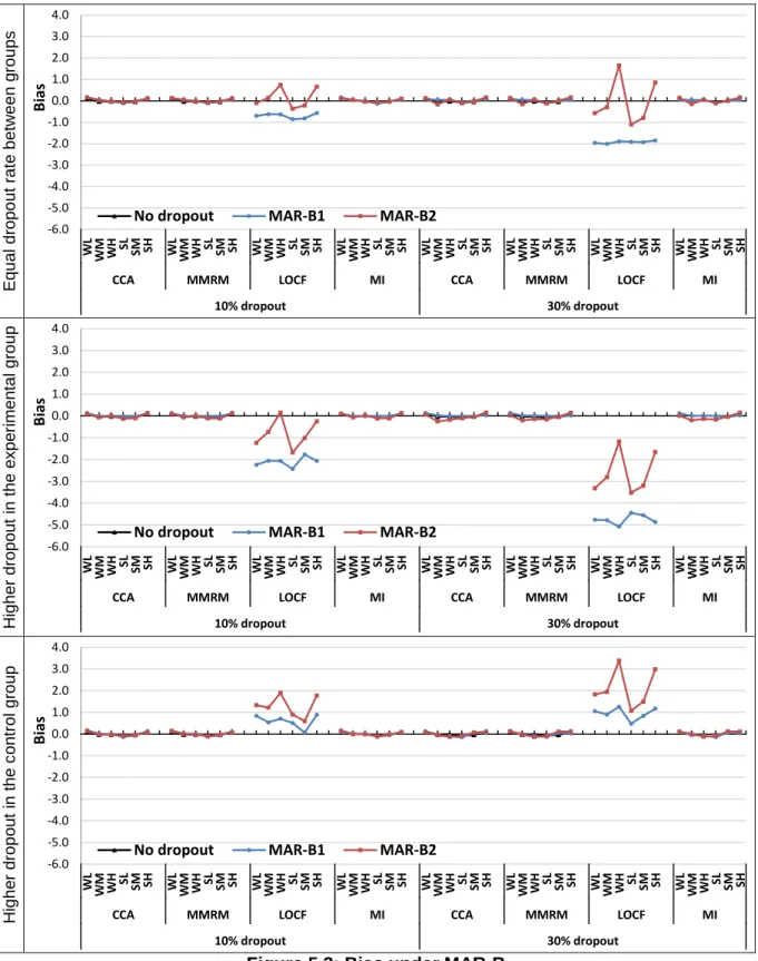
Figure 5.3: Bias under MAR-B ... 117
Figure 5.4: RMSE under MAR-B ... 118
Figure 5.5: Bias under MAR-L... 121
Figure 5.6: RMSE under MAR-L ... 122
Figure 5.7: Bias under MNAR – in relation to (a) level of dropout rate (%) with a fixed strong correlation and moderate SD; (b) data variability and correlation between the repeated assessments with 30% dropout rate ... 125
Figure 5.8: RMSE under MNAR – in relation to (a) level of dropout rate (%) with a fixed strong correlation and moderate SD; (b) data variability and correlation between the repeated assessments with 30% dropout rate ... 126
Figure 5.9: CI coverage under MCAR ... 129
Figure 5.10: Average width of the 95% CI under MCAR ... 130
Figure 5.11: CI coverage under MAR-B ... 132
Figure 5.12: Average width of the 95% CI under MAR-B ... 133
Figure 5.13: CI coverage under MAR-L ... 135
Figure 5.14: Average width of the 95% CI under MAR-L ... 136
Figure 5.15: CI coverage under MNAR – in relation to (a) level of dropout rate (%) with a fixed strong correlation and moderate SD; (b) data variability and correlation between the repeated assessments with 30% dropout rate ... 139
Figure 5.16: Average width of CI under MNAR – in relation to (a) level of dropout rate (%) with a fixed strong correlation and moderate SD; (b) data variability and correlation between the repeated assessments with 30% dropout rate ... 140
Figure 5.17: Statistical power under MCAR ... 143
Figure 5.18: Statistical power under MAR-B ... 145
Figure 5.19: Statistical power under MAR-L ... 147
Figure 5.20: Statistical power under MNAR – in relation to (a) level of dropout rate (%) with a fixed strong correlation and moderate SD; (b) data variability and correlation between the repeated assessments with 30% dropout rate ... 149
Figure 6.1: Effect of trajectory pattern and mean difference between groups over time on bias in estimate of treatment effect ... 155
Figure 6.2: Effect of trajectory pattern and mean difference between groups over time on RMSE of estimate ... 156
Figure 6.3: Effect of trajectory pattern and mean difference between groups over time on coverage of 95% CI ... 157
Figure 6.4: Effect of trajectory pattern and mean difference between groups over time on width of 95% CI ... 158
Figure 6.5: Coverage of 95% CI under various scenarios (MMRM – Mixed model with baseline-as-covariate; cLDA – Mixed model with baseline-as-outcome) ... 162
Figure 6.6: Statistical power under various scenarios (MMRM – Mixed model with
baseline-as-covariate; cLDA – Mixed model with baseline-as-outcome) ... 164 Figure 6.7: Statistical power under different sample sizes (10% dropouts)... 167 Figure 6.8: Statistical power under different sample sizes (30% dropouts)... 168
Figure 7.1: Response rate (%) over time on outcome measures – (a) pain intensity, (b)
PRTEE total score, and (c) SF12 score. ... 187 Figure 7.2: Observed mean profiles according to intervention groups and time at which participants lost to follow-up. ... 189 Figure 7.3: Response rate (%) over time on outcome variables – (a) RMDQ, (b) back pain intensity, and (c) SF12 (PCS & MCS) ... 204 Figure 7.4: Observed mean profile according to intervention groups and the time at which dropped out ... 205
List of abbreviations
ANCOVA Analysis of covariance
ANOVA Analysis of variance
AT As-treated
BOCF Baseline observation carried forward
CCA Complete-case analysis
CI Confidence interval
CONSORT CONsolidated Standards of Reporting Trials
EMA European Medicines Agency
FCS Full conditional specification
FIML Full-information maximum likelihood
FITT Full intention-to-treat
GEE Generalized estimating equations
ICH International Conference on Harmonisation
ITT Intention-to-treat
JM Joint modelling
LME Linear mixed-effects
LOCF Last observation carried forward
MAR Missing at random
MAR-B MAR dependent on baseline
MAR-L MAR dependent on last observed value
MCAR Missing completely at random
MCMC Markov chain Monte Carlo
MCS Mental component score of SF12
MDC Minimum data collection
MI Multiple imputation
MICE Multiple imputation by chained equation
ML Maximum likelihood
MMRM Mixed-effects model for repeated measures
MNAR Missing not at random
MSC Musculoskeletal condition
NAS National Academy of Science
NRC National Research Council
OR Odds ratio
PCM Primary care management
PCS Physical component score of SF12
PITT Partial intention-to-treat
PP Per-protocol
PRTEE Patient-rated tennis elbow evaluation
RCT Randomized clinical trial
REML Restricted maximum likelihood
RMDQ Roland Morris Disability Questionnaire
RMSE Root-mean-square error
SD Standard deviation
SF 12 Short-form 12
TENS Transcutaneous electrical nerve stimulation
wGEE Weighted GEE
List of publications
Royes Joseph, Julius Sim, Reuben Ogollah, Martyn Lewis. A systematic review i.
finds variable use of the intention-to-treat principle in musculoskeletal randomized
controlled trials with missing data. Journal of Clinical Epidemiology 2014 (DOI:
10.1016/j.jclinepi.2014.09.002).
Royes Joseph, Julius Sim, Reuben Ogollah, Martyn Lewis. Evaluation of bias and ii.
precision in methods of analysis for pragmatic trials with missing outcome data: a
Acknowledgements
I would like to thank my supervisors Dr Martyn Lewis, Professor Julius Sim, and Dr Reuben Ogollah for their tremendous support and constructive feedback throughout this study. I am grateful for their invaluable time, advice and encouragement throughout my PhD.
My profound gratitude goes to the Keele University and the Research Institute for Primary Care and Health Sciences for providing the necessary grants and enabling environment that facilitated the timely completion of this thesis. I would also like to thank the TATE and STarT Back trials team for permitting the use of their data.
I would like to thank my family and friends for their support and encouragement.
I am extremely thankful to my wife Smitha Royes and my little son Johan for their encouragement and for being so patient with me all through the programme and, above all, God almighty, the giver of life and grace.
Chapter 1: Introduction
1.1 The present study: research issues
Randomized clinical trials (RCTs) play a vital role in assessing the efficacy and effectiveness of new interventions compared to a standard or control intervention. An
intention-to-treat (ITT) strategy – whereby an analysis should be performed by including
all study participants in the groups to which they were randomized, regardless of any
departures from the original assigned group – serves to preserve the benefits of
randomization, which is intended to ensure that differences in outcome observed between treatment groups are solely the result of the treatments, and to reduce the risk of selection bias. A true ITT analysis requires baseline and outcome measurements on all randomized patients. In practice, no matter how well designed and implemented a study, missing data
are almost inevitable – particularly in pragmatic trials. Different degrees of data
incompleteness in these trials can occur as measurements may be available only at baseline or may be missed for one or several follow-up time-points. In general there are three potential problems that arise from missing data; loss of efficiency, complication in data handling and analysis, and bias due to differences between the observed and unobserved data. Despite extensive literature on methods of handling missing data, it appears that many RCTs continue to be based on inappropriate statistical methods when dealing with missing data (Hollis & Campbell, 1999; Wood et al., 2004; Baron et al., 2005; Gravel et al., 2007; Fielding et al., 2008).
This thesis focused on RCTs with missing continuous outcome data, which are prone to dropouts due to their longitudinal nature. A particular focus is on pragmatic trials of musculoskeletal disorders in primary care (though much of the theory and findings relate more generally to other RCTs). Principally, the work aims to align current recommendations to the methods of analysis being used in practice, and evaluate the
appropriateness of current methods of analysis in respect of the validity in estimation of the true between-group treatment effect conditional on missing data. In order to meet the overall aim, the following objectives were identified.
i. To provide a general overview of the statistical methods to deal with missing data ii. To investigate any divergence among researchers on acceptance of these
methods for analysing missing data
iii. To review current practices being used in the analysis of RCTs in the presence of missing data
iv. To evaluate the impact of various missing data handling methods for the analysis of continuous outcomes in longitudinal clinical trials under various plausible conditions in a comprehensive manner using simulation studies
v. To propose and investigate how reminder responses – data that are retrieved by
sending reminders to the initial non-responders – can be utilized to infer the nature of missing data and help inform appropriate analysis of the RCT dataset in order to reduce potential bias in treatment effect estimation
vi. To collectively appraise the various findings and provide recommendations on how to deal with missing data in RCTs
1.2 Outline of thesis
Chapter 2: Background
Chapter two provides an initial background to the issues associated with missing data and a summary of the current missing data literature. In particular, the review focuses on key issues relating to missing continuous outcome data and methods of handling missing data currently in use in longitudinal clinical trials. The methods include listwise deletion, single imputation (e.g. last observation carried forward method [LOCF]), multiple imputation (MI), and a maximum likelihood based approach (e.g. mixed-effects model for repeated measures [MMRM]) that can use all available data without imputation. This chapter discusses the advantages and disadvantages of these missing data methods based on a review of previous simulation studies that compared these methods. The chapter also discusses the limitation of these simulation studies and rationalizes the requirement for further study.
Chapter 3: Systematic review
In this chapter, I present a systematic review that examines current practice relating to ITT analysis and methods to handle missing data in published trials. Specifically, the review has the following objectives:
To describe the extent of adherence to random allocation;
To describe the extent of reported dropout;
To summarize the frequency in use of different analytical methods used to handle
missing data;
To assess the use of sensitivity analyses used to assess the robustness of the
In this study, the review focuses on RCTs reported in five leading medical journals that mainly focus on research in musculoskeletal conditions.
Chapters 4–6: Simulation study
Chapter four details the methodology of a simulation study that investigates the performance of various methods for handling missing data in a longitudinal clinical trial with continuous outcome data, across a number of different scenarios. The methods include listwise deletion, LOCF, MI, and MMRM. The simulation study has the following objectives:
To assess the relative performance of the missing data methods with respect to
bias and accuracy of the estimate of treatment effect under various scenarios;
To assess the relative performance of the missing data methods with respect to
the coverage of confidence interval of the estimate of treatment effect at the nominal alpha level of 0.05 under various scenarios;
To assess the relative performance of the missing data methods with respect to
conditional loss of statistical power to detect the true treatment effect under various scenarios (given nominal power of 90%);
To assess whether an increment in sample size in proportion to an expected
dropout rate helps to achieve the required statistical power when using these missing data methods;
To assess whether including the baseline measure as part of the response vector
in an MMRM model has an advantage over including it as a covariate.
Chapter 7: Re-analysis of real incomplete longitudinal RCT datasets
Chapter seven presents the re-analysis of two pragmatic clinical trials that included a reminder process for non-responders. Here, I propose an approach that utilizes the reminder process as a proxy for missingness to assess the impact of missing data on the estimation of treatment effect, and the likely missing data mechanism.
Chapter 8: Discussion and conclusion
Chapter eight concludes with a detailed discussion and interpretation around the findings from all the chapters. I finish by providing a summary of my recommendations on how to deal with missing data in RCTs, and some thoughts on further research in this area.
Chapter 2: Background
2.1 Introduction
This chapter focuses on key issues relating to missing continuous outcome data and methods of handling the missing data currently in use in longitudinal clinical trials. This chapter also discusses the advantages and disadvantages of these missing data methods based on a review of available simulation studies that compared these methods. The chapter further discusses the limitation of these simulation studies and then conclude by identifying the need for a further study to compare these missing data techniques. Before describing the different missing data techniques, the definition and underlying theory of missing data are also presented.
2.2 The problem of missing data in clinical trials
Randomized clinical trials (RCTs) play a vital role in assessing the efficacy and effectiveness of new interventions compared to a standard or control intervention. Randomization in a clinical trial is intended to generate comparable groups of patients in terms of known and, more importantly, unknown factors that could be associated with the outcome of interest at the onset of the trial. That is, the method ensures at least theoretically, that both observed and unobserved baseline differences between the interventions are attributable to chance. After accounting for chance variations, the remaining differences can be attributed reliably to the interventions so long as other sources of bias have been eliminated. To provide an unbiased comparison of estimates of treatment effects, randomization alone is not sufficient and it is also important to obtain outcome measurements on all randomized patients. Therefore, the principal advantage of randomization is threatened when some outcome measurements are missing. As trials with missing data may not retain the balance of randomization, the basis for statistical inference is lost (Wright & Sim, 2003; Lewis & Machin, 1993) and there is no longer a
statistical rationale to guarantee lack of bias for the estimation of the parameter and its associated confidence interval – even if the study is assumed to be free of other risks of bias, such as non-masked evaluation.
The intention-to-treat (ITT) principle is widely recommended as the primary design and analysis strategy for clinical trials (Frangakis & Rubin, 1999; Feinman, 2009); this is mandatory for any confirmatory trial (Committee for Proprietary Medical Products, 2001; Food and Drug Administration, 2008). An ITT analysis is a pragmatic approach that may help to avoid bias in estimation of treatment effect occasioned by any study protocol violation after randomization, such as dropout of subjects, which may affect the baseline equivalence established by randomization (Schwartz & Lellouch, 2009). An ITT analysis corresponds to analysing groups exactly as randomized. Strictly, an ITT analysis should include all randomized subjects, regardless of their adherence with the eligibility criteria, the treatment they actually received, and subsequent withdrawal or loss to follow-up from treatment or deviation from the study protocol (Fisher et al., 1990). Accordingly, an ITT analysis includes all randomized subjects according to randomized treatment assignment. It ignores protocol deviations, non-compliance, withdrawal and anything that happens after randomization (Heritier et al., 2003; Kruse et al., 2002). An ITT analysis is generally
explained as “once randomized, always analysed” (Wertz, 1993). Hollis and Campbell
(1999) point out two purposes of an ITT approach: firstly, it maintains treatment groups that are similar apart from random variation, and secondly, it allows for non-compliance and deviations from policy by investigators. Thus, an ITT analysis reflects the practical clinical scenario. Therefore, an ITT analysis is most suitable for pragmatic trials, which measure the effectiveness of treatments in everyday practice (Hollis & Campbell, 1999).
It has been reported that investigators often refer to ITT to describe the analysis of all available subjects as randomized without considering the issue of missing data (Gravel et al., 2007). It is pointed out in the CONSORT (CONsolidated Standards Of Reporting
Trials) statement that a strict ITT analysis is often hard to achieve for two main reasons: (i) missing outcomes for some participants and (ii) non-adherence to the treatment protocol (Moher et al., 2010). Therefore, compliance with the ITT principle would necessitate complete follow-up of all randomized subjects for study outcomes and retention of randomized allocation grouping regardless of deviation from treatment protocol. Exclusion of participants, possibly in a non-random or informative way, raises great concerns about the validity of the study. Many reviews of RCTs concede that the ITT approach is often inadequately described and applied (Schulz et al., 1996; Hollis & Campbell, 1999; Kruse
et al., 2002; Gravel et al., 2007) – the deviation from the true ITT was mostly linked in
these reviews with missing data (Chapter 3). The International Conference on
Harmonisation (ICH) guideline (Food and Drug Administration, 1997) states: “no analysis
should be considered complete unless the potential biases arising from these specific exclusions, or any others, are addressed.”
RCTs are generally longitudinal in nature – such that the outcome of interest is measured
at more than one occasion – with a common schedule of measurements for all
participants, but with a small number of measurement occasions. In a review of trial reports published between July and December 2001 in four major general medicine
journals (BMJ, JAMA, Lancet and New England Journal of Medicine), among the 71 trial
reports that were examined, 37 (52%) of them were with multiple follow-up assessments (Wood et al., 2004). Even though outcome data are observed in a longitudinal fashion, the
primary focus of RCTs is often a specific time of measurement, usually the last – called
the primary endpoint. The aim of these trials is usually limited to comparing the effect of two or more treatments at this specific time-point – i.e., estimating treatment effect at the primary endpoint (Verbeke & Molenberghs, 2005). Importantly, many musculoskeletal conditions (MSCs) necessitate long-term trials because they are chronic conditions, and this consequently results in a high number of patients being discontinued from the trial
prior to the primary endpoint (Kim, 2011; Moore et al., 2008); however, there is often at least one post-baseline assessment among these missing follow-ups.
Missing data, a common problem and a potential source of bias in research, involves information that is missing for some variable(s) and/or for some unit(s) of observation (Allison, 2001). In this thesis, missing data are defined as the absence of some value(s) on an outcome variable. Missing data also occur in the covariates but that is not the focus of this thesis. In practice, no matter how well designed and implemented, there will almost always be some missing data (Crutzen et al., 2013). Within RCTs, outcome data can be missing due to several reasons (Little & Rubin, 2002). For example, in a trial (Baerwald et al., 2010) with a 24% (191/810) dropout rate, reasons for the dropouts included lack of efficacy (n=63), adverse events (n=55), withdrawn consent (n=39), violation of eligibility criteria (n=18), loss to follow-up (n=7), and other unspecified reasons (n=9). A positive outcome, such as symptom relief, recovery, or cure, may also lead to discontinuation from a trial (National Research Council, 2010). Reasons for the dropouts are extremely important and should be collected, since they can be used to justify the assumptions of
statistical analysis. Moore et al. (2008) examined participants’ discontinuation in clinical
trials based on 21 trial datasets in MSCs (osteoarthritis, rheumatoid arthritis, chronic low-back pain and ankylosing spondylitis) and reported that lack of efficacy or intolerable adverse events, or both, were the major reasons for discontinuation in those trials.
The validity and interpretability of findings from RCTs can be substantially reduced by missing data (Little & Rubin, 2002; Molenberghs & Kenward, 2007; European Medicines Agency, 2010; National Research Council, 2010; Fleming, 2011). In an RCT, as mentioned earlier, the advantages of randomization are jeopardized when the trial has missing data. To prevent selection bias in a clinical trial, it is important to adopt an ITT strategy, which requires all randomized patients to be included and analysed as randomized. However, the presence of missing data in a trial creates many challenges in
the selection of an ITT sample. The impact of missing data in a study is difficult to assess and is related to the question of what would hypothetically have been observed if no patient had withdrawn from the study. In general, there are three potential problems associated with the presence of missing data: loss of efficiency, bias in estimate of true parameters, and complication in data handling analysis (Horton & Lipsitz, 2001).
Loss of efficiency is an unavoidable consequence of missing data. Trials with missing data will be underpowered because fewer participants have completed than was originally planned; that is, the trial no longer has enough participants to demonstrate the same level of clinically important differences as statistically significant (Little & Rubin, 2002; Molenberghs & Kenward, 2007).
Another implication is that ignoring the presence of missing outcome data may lead to biased estimates, and thereby misleading inferences about treatment effects (Molenberghs & Kenward, 2007). A major concern is that being lost to follow-up could be related to a patient’s responses to the treatment. Participants who do not complete a trial of a new treatment, for example, may be: those who improved the most, and do not see the necessity of continuing; those who improved the least, and see no reason to continue to comply with the treatment that is not working for them; or those who may have decided to discontinue owing to the occurrence of adverse effects. If the majority of dropouts are those who improved, then this will serve to make the interventions appear less effective than they actually are. Conversely, if most of the people dropped out because the new treatment was ineffective, this will, paradoxically, make the intervention look better, because many of the non-responders are no longer in that arm of the study. In view of the fact that missing data usually occur for reasons outside of the control of the investigators, and may be related to the outcome measurement of interest, the subsequent data analysis is extremely complicated.
As noted previously, no analysis should be treated as appropriate unless potential biases due to missing data are appropriatly addressed. To address this issue either imputation of values or modelling for missing data is generally required (European Medicines Agency,
2010), which rely heavily on untestable assumptions about the missing data – the wrong
assumptions lead to biased estimates of treatment effect and standard errors. Since the potential impact of missing data depends primarily on missing data assumptions, it is important to investigate the processes (i.e. missing data mechanism) leading to missing data (Rubin, 1976; Little & Rubin, 2002).
2.3 Missing data: theoretical framework
To understand how best to deal with missing data, the first step is to determine the nature of the missing data and their possible implications for statistical inferences (National Research Council, 2010). The validity of any statistical analyses of incomplete data depends critically on causes of missing data. Since observed data cannot themselves explain definitely what might be the reasons for the missing data, it is necessary to make assumptions about the missing data mechanism. Therefore, statistical inferences on incomplete data rely on the subjective, untestable assumption about the distribution of missing data. Little and Rubin (1987; 2002) described a general missing data taxonomy, which includes a useful hierarchy of missing data mechanisms based on possible causal relationships between missing data and observed data in a study. Further discussions around this taxonomy for missingness in longitudinal data are available (Little, 1995; Schafer & Graham, 2002). A detailed review of this taxonomy is followed by an introduction of the repeated measures data structure.
Let refer to a vector of repeated measurements of an outcome variable
on occasions, and as design variables that represent treatment indicators and
baseline covariates. For simplicity, it is assumed that is fully observed. To distinguish
whether is missing, where if observation at the th time for the th subject is missing.
2.3.1 Missing data patterns
In longitudinal studies, missed visits and/or study dropouts resulting in missing response data may occur. A missed visit occurs when a participant misses a clinic visit or fails to respond to a questionnaire meant for a particular follow-up visit during a follow-up schedule, whereas a dropout occurs when a participant discontinues from the study at any time during the study period and thus fails to provide outcome data thereafter. In trials with repeated follow-ups, participants who miss a study visit are often lost thereafter (National Research Council, 2010).
A dataset with a series of measurements on an outcome variable is
said to have a monotone missing pattern when an event that a measurement is missing
for an individual implies that all subsequent measurements , are missing for that
individual. That is, under a monotone missing data pattern, the reason for missing data in a longitudinal trial is solely through study dropouts. Figure 2.1 shows a representation of monotone and non-monotone missing data patterns. A dataset with an arbitrary missing pattern is one with a monotone and non-monotone (i.e. intermittent) missing pattern; the missing data are due to both missed visits and study dropouts.
Monotone missing patterns Non-monotone missing patterns
ID Y1 Y2 Y3 Y4 1 o o o o 2 o o o m 3 o o m m 4 o m m m ID Y1 Y2 Y3 Y4 1 o o o o 2 o m o m 3 o o m o 4 o m m o
‘o’ – observed; ‘m’ – missing
2.3.2 Missing data mechanism
To understand the potential impact and how best to deal with missing data it is important to consider the process (i.e. mechanism) leading to the missingness. A general taxonomy for missing data, which is common in the statistical literature (Rubin, 1976; Little & Rubin, 1987; 2002; Little, 1995; Schafer & Graham, 2002; National Research Council, 2010), distinguishes between missing data that are missing completely at random (MCAR), missing at random (MAR), and missing not at random (MNAR). The classification is based on the dependence of missingness on observed and/or unobserved data. The missing
data mechanism can be represented in terms of conditional distribution for the
missing data indicators given the values of the study variables that were intended to be collected.
Missing data are MCAR if missingness is independent of observed and unobserved data
(i.e., missingness does not depend on values of the variables and ). That is,
. This is the most desirable, but an unlikely scenario in trials with missing data. An example of such a scenario occurs when a participant discontinues a trial due to change of location during the course of the trial for reasons unrelated to the trial and/or disease of interest (e.g. job transfer). DeSouza et al. (2009) point out that missed visits are often not study-related, and thus the missing data are MCAR.
The second classification, which is more realistic than MCAR, is MAR. This mechanism
requires that missingness is dependent on observed responses and/or covariates ( ),
but independent of unobserved responses ( ). That is, . This
type of missingness may be referred to as outcome-dependent MAR and/or covariate-dependent MAR, as the case may be (DeSouza et al., 2009). In longitudinal studies, MAR is plausible as dropouts are more likely to be related to previous responses (DeSouza et al., 2009). For example, if participants withdraw from a chronic pain trial once their pain intensity exceeds a certain threshold, then the missing data are MAR. The plausibility of
the MAR assumption can be improved by considering auxiliary variables that are predictive of whether the outcome variables are missing and predictive of the values of the missing variables (National Research Council, 2010).
MAR will fail to hold if missingness is dependent on unobserved data after accounting for available observed data. In that situation, the missingness is said to be MNAR. That is, . For example, if a participant feels better on his or her clinical condition after a visit and decides not to show up for the next scheduled visit, then the missing data are MNAR. Consequently, in longitudinal studies, future values of outcome variables for those who drop out cannot be reliably predicted based on data collected prior to dropping out if MNAR holds.
The implication of MCAR is that a missing data mechanism need not to be incorporated into an inference model, and a valid analysis is possible with observed data alone. For MAR, the missing data mechanism can be considered ignorable after including correlates of missingness in an inference model. For MNAR, on the other hand, the missing data mechanism is non-ignorable and needs to be incorporated into an analysis to make a valid inference. Importantly, a particular missing data mechanism is not in itself always ignorable or non-ignorable, depending on the statistical model. That is, if a statistical model fails to incorporate correlates of missingness, then a missing data mechanism cannot be considered as ignorable. Therefore, it is important to obtain additional variables that explain missingness and include these variables into the statistical model. As discussed here, missing data mechanisms play an important role in determining appropriate formal statistical analyses of data with missing values; however, it is difficult to distinguish the mechanisms in practice. In fact, on the basis of the observed data alone, it is impossible to identify the underlying missing data mechanism with certainty (Fielding et al., 2009).
2.3.3 Identification of the missing data mechanism
Few methods have been proposed to test for MCAR as a preliminary screening tool (Little, 1988; Diggle, 1989; Ridout, 1991; Fairclough, 2002). The purpose of these methods is not to explicitly detect violations of MAR, but violations of MCAR by identifying dependence on observed data. For example, Fairclough (2002) describes a logistic regression approach to confirm that a dropout process in repeated measurement data depends on observed data. A significant association between the dropouts and the observed data serves to rule out the possibility of MCAR.
Since there are valid analysis methods available for MAR data and not for MNAR data, the important consideration is the distinction between MAR and MNAR rather than between MCAR and MAR. To distinguish between MAR and MNAR, one must examine the relationship between missingness and unobserved data. Although it is impossible to determine the relationship empirically, a method has been proposed to evaluate the possibility of MNAR through a comparison of immediate responders who responded without any reminders and reminder responders who responded after sending reminders. By treating reminder responses as missing, Fielding et al. (2009) outlined an extension of Fairclough’s logistic regression approach to determine whether the mechanism behind the reminder data are MNAR rather than MCAR or MAR. A significant difference in current scores between immediate and reminder responders after adjusting for the covariates that are predictors of reminder responses constitutes evidence of possible MNAR data. However, this evaluation excludes cases with actual missing responses.
2.4 Methods for handling incomplete continuous data
Several statistical procedures exist for handling missing data. These procedures can generally be divided into three broad categories: procedures based on listwise deletion; imputation-based procedures; and model-based procedures. Procedures based on
listwise deletion simply discard cases with missing values and analyse only those cases with complete data on all variables included in an analysis model. Analysis of covariance (ANCOVA), which is the most commonly used analysis method to estimate treatment effect in an RCT setting (Chapter 3), leads to listwise deletion of cases with missing data unless the missing values are imputed. In imputation-based procedures, missing values are replaced with particular values, which are determined by a specific procedure, in order to secure a complete dataset for analysis. As Little and Rubin (2002) explain, the purpose of imputation is to preserve important data characteristics, such as mean and variance, of the whole dataset but not to predict the true values of the missing data. From that perspective, a method that can replace missing values with multiple plausible values has
been proposed (Rubin, 1978). Lastly, model-based procedures allow available data – not
leading to listwise deletion – without imputation of missing values.
2.4.1 Description of candidate approaches to analysing longitudinal RCT data
with missing values
2.4.1.1 ANCOVA without imputation of missing values
In an RCT, a transient benefit shown early in the trial might not persist through to the end of the trial and therefore it is necessary to demonstrate a sustained improvement at the primary endpoint. Although outcome data are commonly measured at more than one follow-up in trials, the aim of these trials is therefore usually limited to comparing the effect of two or more treatments at a specific time-point (Verbeke & Molenberghs, 2005). Unless it is important to know how study participants have reached the study endpoint, a simple comparison of the treatment groups at the primary endpoint is often recommended and adequate to demonstrate the treatment effect, if any (European Medicines Agency, 2006; Verbeke & Molenberghs, 2005). In case of continuous outcomes, a standard ANCOVA model, with baseline values of the outcome as the covariate, would be sufficient for such a comparison if outcome data are available on all participants (Van Breukelen, 2006;
Egbewale et al., 2014). Alternative methods such as analysis of variance and change-score analysis are not recommended because these analysis methods are subject to bias and are less precise than ANCOVA in relation to pretest-posttest correlation and the direction of baseline imbalance (Egbewale et al., 2014).
ANCOVA utilizes baseline and observed covariates as predictor variables in an analysis model, with the follow-up outcome at the primary endpoint as the outcome variable. For
subject and repeated observations at visit (primary endpoint) per
subject, the ANCOVA model is
where
: outcome measurement at the primary endpoint for the th subject
: outcome measurement at baseline for the th subject
: intercept
: effect of baseline measurement ( )
: effect size at the primary endpoint
: treatment group for subject
: assumed to be independently distributed from a univariate normal distribution
When employing ANCOVA, only subjects with complete observations on all the variables of interest are included in the model. This kind of approach is referred as complete-case analysis (CCA) in missing data literature. In this method, cases with missing data on any variable of interest are dropped from the analysis (i.e., listwise deletion of subjects with missing data). For example, Hewlett et al. (2011) investigated the effect of group cognitive-behavioural therapy compared to the control intervention on fatigue impact
among people with rheumatoid arthritis. The primary outcome – fatigue impact visual
analogue scale – was measured at baseline, week 6, week 10 and week 18 (primary
endpoint), and the study failed to measure the outcome on 33% (42/127) of participants at the primary endpoint. The primary analysis using ANCOVA removed those 42 participants irrespective of whether the outcome data were observed at earlier times. That is, the study analysed only a subset of participants. This generally does not provide a valid estimator of an ITT estimate (National Research Council, 2010). CCA requires the assumption that missing data are a random subset of the population of interest (Little & Rubin, 2002). Accordingly, if the missing data are MCAR, the sub-sample will be a random sample of the original sample, and the results of CCA will be unbiased but inefficient because of an inflated standard error if missingness is appreciable (Little & Rubin, 2002). However, if the missing data are MAR or MNAR, the analysis using CCA may not be valid as the reduced sample may no longer be representative of the population of interest, giving rise to biased estimates. In spite of these limitations, listwise deletion is still popular among researchers (Chapter 3) and is the default option with many statistical methods in major statistical software packages.
2.4.1.2 ANCOVA with single imputation of missing values
Single imputation methods replace each missing data point with a single value in order to produce a complete dataset to which standard statistical methods, such as ANCOVA, can be applied without discarding subjects with missing observations. That is, these methods treat imputed values as real values, and hence do not account for the uncertainty around the missing values. Therefore, the variance of estimates is likely to be too small, leading to underestimation of standard error. Further, these methods may produce biased estimates depending on how far the imputed value differed from the true value, which is unknown in real data. Hence, inferences based on the filled-in data can be distorted if the assumptions underlying the imputation method are invalid. Commonly, the imputation of
missing observations is based on the observed values. Several ad hoc strategies to
perform single imputations – such as last observation carried forward (LOCF), mean
imputation and regression imputation – are common in practice (Chapter 3).
Imputing by LOCF is a common single imputation method for repeated measures. In this method, a missing outcome value is replaced with the most recently available value of that outcome variable. LOCF therefore makes a strong assumption that there is no change in outcome for a participant after dropout. The rationale of this approach is that it is fairly conservative, as this approach likely underestimates the degree of change in an outcome over time (Streiner, 2008). However, this may not necessarily be the case in estimating a treatment effect (i.e. between-group difference in change) in trials, since imbalance between treatment groups in underestimation of degree of change in the outcome may overestimate the treatment effect. For example, if many participants who are expected to do worse over time discontinue a study treatment, or many of those who are expected to do well over time discontinue a control treatment, the benefit of the study treatment is more likely to be overestimated than the control with the LOCF method.
Some researchers contend that LOCF makes an MCAR assumption. For example,
Mallinckrodt et al. (2008) state “when assessing LOCF mean change via analysis of
variance (ANOVA), the key assumptions are that missing data arise from an MCAR mechanism and that for subjects with missing endpoint observations, their responses at the endpoint would have been the same as their last observed values”. However, the assumption of no change in outcome after drop out may not be valid under MCAR or MAR (National Research Council, 2010). As mentioned earlier, the MAR assumption is that the
predictive distribution of an outcome variable at time ( ) conditional on design variable
and observed data is the same for both observed and missing . However,
assumption may not hold with observed (i.e. the probability may not be one for the observed data). That is, in general LOCF makes an MNAR assumption.
2.4.1.3 ANCOVA with multiple imputation
Multiple imputation (MI) is designed to substitute each missing value with a range of plausible values based on observed information in order to reflect the uncertainty associated with imputation of missing values (Rubin, 1978; 1987; 1996; Schafer, 1997; Little & Rubin, 2002; Molenberghs & Kenward, 2007; Carpenter & Kenward, 2013). For example, in a study with two observations (age and pain intensity) on each participant, suppose that age is completely observed and pain intensity is incomplete. The basic idea is to use the association between age and pain intensity from the complete data to fill the missing pain intensity score with multiple plausible values. These multiple values are a random draw from the posterior predictive distribution of missing values based on a statistical model explaining the association between the variables. The imputation is based on an implicit and untestable assumption that the association between age and pain intensity is the same for those participants who provided complete data and those who do not. That is, MI requires the MAR assumption.
The MI procedure involves three stages (Rubin, 1987): imputation, analysis and pooling. Initially, it is required to specify a statistical model (referred to as an imputation model) to explain the relationship between observed data and missing data. The posterior distribution for the estimated parameters of the model is used to simulate the parameters
of the posterior predictive distribution of the missing data from which m predicted values
are drawn. This creates m completed datasets. In the second stage, one fits a statistical
model (referred to as analysis model), e.g. ANCOVA model, to each completed dataset,
and generates parameter estimates ̂ ̂ ̂ and associated variance. Finally, these
rule (1987). The MI estimate is the average of the estimates from the datasets, and the variance of the estimate is
( )
where is the average of the variances from the m datasets and is the
between-sample variance of the estimates over the m datasets.
Methods for MI of multivariate missing data include three broad approaches (Molenberghs & Kenward, 2007): (i) sequential MI for data with monotone missingness; (ii) joint modelling (JM) approach, which assumes that all variables in the imputation model jointly follow a multivariate normal distribution; and (iii) full conditional specification (FCS) approach (which is referred to as multiple imputation by chained equation [MICE]), which does not rely on the multivariate normality assumption. If the missing data pattern is monotone, regression imputation can be performed sequentially, starting with the variable having least missing values; this approach uses noniterative techniques for simulating from the posterior predictive distribution of missing data. The imputation method based on a multivariate normal regression uses an iterative Markov chain Monte Carlo (MCMC) technique to simulate from the posterior predictive distribution of missing data. The MICE method uses a Gibbs-like algorithm to obtain imputed values. If the missingness mechanism is non-monotone, both JM and FCS approaches are generally preferred and provide similar results in a standard regression analysis involving a mixture of continuous and categorical variables (Lee & Carlin, 2010).
2.4.1.3.1 Selecting variables for an imputation model
As mentioned earlier, MI requires two statistical models: an imputation model, which is used to impute missing values and a substantive analysis model, which is used to analyse the imputed data. Choice of imputation model for the MI can have a pronounced effect on
the outcome of the data analysis (Spratt et al., 2010). Ideally, an imputation model should include all variables that are in the substantive analysis model and should reflect the structure of the subsequent analysis (Kenward & Carpenter, 2007; Sterne et al., 2009;
Carpenter & Kenward, 2013) – which is referred to as a restrictive modelling strategy
(Collins et al., 2001). Further, it is possible to incorporate auxiliary variables that are not part of the analysis model into the imputation model in order to make MAR more plausible and, therefore, to increase efficiency and reduce bias (Collins et al., 2001; Spratt et al., 2010) – which is referred to as an inclusive modelling strategy (Collins et al., 2001). White et al. (2011b) pointed out that one should include in an imputation model all variables that predict the incomplete variables in an analysis model and/or predict whether the observations on the incomplete variables are missing.
2.4.1.3.2 Selecting the number of imputations
The amount of missing data should be considered when deciding the number of
imputations, say m, in the MI method. Rubin (1987) previously demonstrated the relative
efficiency of a finite-m estimator as ̅̅ ( ) , where is the fraction of missing
information for an outcome measure to be analysed. Using this formula, table 2.1 shows
the relative efficiencies with different and fractions of missing information.
Table 2.1: Percent efficiency of MI estimation Rate of missing data ( )
0.1 0.3 0.5 0.7 0.9 1 91 77 67 59 53 3 97 91 86 81 77 5 99 94 91 88 85 10 99 97 95 93 92 100 100 100 100 100
Following Rubin’s calculation of relative efficiency, many researchers have advocated a small number of imputations as adequate to yield excellent results. For example, Schafer and Olsen (1998) suggested only 2–5 imputations, and Schafer (1999) further emphasised that no more than ten imputations are usually required. However, these suggestions have been recently critiqued. Graham et al. (2007) and Spratt et al. (2010) observed that, with the small number of imputations, variability due to the imputation procedure was substantial enough to affect inferences, and recommend that many more imputations should be performed than previously considered adequate. In favour of this recommendation, White et al. (2011b) proposed a rule of thumb, which states that the number of imputations should at least be equal to the percentage of incomplete cases.
2.4.1.4 Model-based methods: direct maximum likelihood estimation
Maximum likelihood (ML) refers to a method of estimating the parameters of a statistical model. ML estimates, which maximize the likelihood function of sample data, are asymptotically unbiased if the model has been specified correctly (Little & Rubin, 2002). When data is incomplete, direct likelihood based methods (also referred to as full-information ML [FIML] methods) can use all available data, instead of deleting observations with missing values, for analysis without explicit imputation of missing data, and assume that the missing data mechanism is either MCAR or MAR (Little & Rubin,
2002). The joint likelihood for the observed data yobs and the missing data indicator is:
if MAR
Thus, if the parameters and are distinct, then can be estimated by maximizing the
observed data likelihood (yobs; θ) alone, independent of the model for . Therefore, when
the missingness mechanism is MCAR or MAR, specification of a missingness model is unnecessary and inferences are based on the likelihood function given the observed data only (DeSouza et al., 2009). In addition to the MAR assumption, FIML methods require a large sample size and need to meet the multivariate normality assumption for the variables used in a model (Little & Rubin, 2002).
2.4.1.4.1 Mixed-effects models (Random-effects models)
For longitudinal data, mixed-effects models provide a parsimonious way to specify a multivariate distribution. Linear mixed models are an extension of linear regression models allowing for inclusion of random-effects to account for within-subject dependency in the longitudinal measurements (Laird & Ware, 1982). Specification of mixed-effects models requires: (i) a model for the mean structure of the longitudinal data, which usually depends on covariates, design matrix for time, treatment group and patient specific random-effects; (ii) an assumption on the distribution of the random-effects; and (iii) specification of an additional correlation matrix in the longitudinal measurements (Wong et al., 2011). The model can be specified as
, where
is the x 1 vector of responses for subject , and is the number of
measurements for subject (
is a known x covariate matrix of th subject for fixed effects
is a known x covariate matrix of th subject for random effects
is a x 1 vector of unknown subject effects (random-effects) distributed as
is a x 1 vector of random residuals distributed independently as
and are independent
In matrix notation, = ( ) and = ( ) represent the
variance-covariance matrices of and respectively. Therefore, the variance-covariance matrix for
the vector of outcomes for all subject visits is specified as:
2.4.1.4.2 Mixed-effects model for repeated measures using categorical time
effects (MMRM)
Likelihood-based, mixed-effects models offer a general framework to extend the standard ANCOVA for repeated measures data in a clinical trial to provide the direct estimates and statistical test for treatment group differences at the primary endpoint, which is typically of direct interest for regulatory decision-making, while incorporating available data for participants who dropped out early (Mallinckrodt et al., 2001a). In many longitudinal RCT settings, the repeated measures are balanced in the sense that outcomes are assessed at the same time interval over a limited number of visits for all participants. This allows a “saturated” mixed-effects model to be specified by including a full treatment group by measurement time interaction for outcome means combined with an unstructured
within-subject error variance-covariance matrix1 (Beunckens et al., 2005). The model is often
1
An unstructured within-subject error variance-covariance matrix is recommended unless the underlying (“true”) structure is known (Mallinckrodt et al., 2004)