Outlier preservation by dimensionality reduction techniques

Outlier Preservation by

Dimensionality Reduction Techniques

Martijn Onderwater

1

_{Center for Mathematics and Computer Science (CWI)}

Science Park 123, 1098 XG, Amsterdam,

The Netherlands.

E-mail: [email protected]

Fax: +31 (0)20 592 4199

_{VU University, Faculty of Sciences}

Amsterdam, The Netherlands.

_{Corresponding author}

September 24, 2013

IJDATS - 8740

Abstract

Sensors are increasingly part of our daily lives: motion detection, light-ing control, and energy consumption all rely on sensors. Combinlight-ing this information into, for instance, simple and comprehensive graphs can be quite challenging. Dimensionality reduction is often used to address this problem, by decreasing the number of variables in the data and looking for shorter representations. However, dimensionality reduction is often aimed at normal daily data, and applying it to events deviating from this daily data (so-calledoutliers) can affect such events negatively. In particular, outliers might go unnoticed.In this paper we show that dimensionality re-duction can indeed have a large impact on outliers. To that end we apply three dimensionality reduction techniques to three real-world data sets, and inspect how well they preserve outliers. We use several performance measures to show how well these techniques are capable of preserving outliers, and we discuss the results.

Keywords: dimensionality reduction; outlier detection; multidimensional scaling; principal component analysis; t-stochastic neighbourhood em-bedding; peeling; F1-score; Matthews Correlation; Relative Information Score; sensor network.

Biographical notes: Martijn Onderwater is a Ph.D. student at the Center for Mathematics and Computer Science (Amsterdam, The Nether-lands), and at VU University (Amsterdam, The Netherlands). He received a M.Sc. degree in Mathematics (2003) from the University of Leiden (The Netherlands), and a M.Sc. degree in Business Mathematics & Informatics (2010, Cum Laude) from VU University Amsterdam. He also has sev-eral years of commercial experience as a software engineer. His research focuses on sensor networks, and his interests include dimensionality re-duction, outlier detection, caching in sensor networks, Markov decision processes, correlations in sensor data, and middleware for sensor networks.

1

Introduction

Recent technological developments have resulted in a broad range of cheap and powerful sensors, enabling companies to use sensor networks in a cost-effective way. Consequently, sensor networks will increasingly become part of our daily life. One can for instance envision a house with sensors related to smoke de-tection, lighting control, motion dede-tection, environmental information, security issues, and structural monitoring.

Combining all this information to actionable insights is a challenging problem. For instance, in the event of a burglary in a house, the sensors involved in motion detection, environmental monitoring, and security all yield useful information. Providing a short insightful summary that helps users identify the event and take appropriate action is essential. Dimensionality reduction (dr) is a family of techniques aimed at reducing the number of variables (dimensions) in the data and thus making the data set smaller. In essence, it helps identify what is important, and what is not.

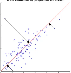
However, in practise dimensionality reduction often yields some loss of informa-tion, and applications might be affected by this loss. For instance, the burglary mentioned before is a (hopefully) rare event that is different from normal pat-terns in the sensor data (i.e. a so-called outlier). Unfortunately, _dr-methods often lose outliers among the regular sensor data. Figure1illustrates this situ-ation using a two-dimensional data set with an outlier near the top-left corner. When dimensionality is reduced by projecting all points onto a line, the outlier is mapped into the center of the reduced data set (the middle arrow in Figure

1), and is thus no longer an outlier. So dimensionality reduction might lose outliers among regular points, causing problems for applications relying on the

−2 −1 0 1 2 3 4 −2 −1 0 1 2 3 4

Data reduction by projection on a line.

x

y

Figure 1. A two-dimensional data set reduced to one dimension, with an outlier (middle arrow) mapped to the center of the reduced data set

detection of outliers. The example in Figure1illustrates onedr-technique, but many others exists, each affecting outliers differently.

In this paper we show that dr-techniques affect outliers, by measuring their capability to preserve outliers. For this purpose we describe three well-known

dr-techniques that are relevant for a broad audience, and apply them to several

real-world data sets from a sensor-related context. For each _dr-technique we capture its capability to preserve outliers in three performance measures, and compare the results. From the three techniques we will identify the one with the best performance, and discuss the intuitions behind the scores.

Research on both dimensionality reduction and outlier detection is abundant. An overview of dimensionality reduction techniques can be obtained from Carreira-Perpinán(1997);Fodor(2002);Gupta and Kapoor(2012);Kline and Galbraith

(2009);Onderwater(2010);Van der Maaten et al.(2009). For outlier detection, we refer readers to, e.g., Agyemang et al. (2006); Hodge and Austin (2004);

Maalouf and Trafalis(2011);Zhang et al.(2010, 2007). Certain specific topics such as intrusion detectionGogoi et al.(2011) and fraud detectionBecker et al.

(2010);Phua et al.(2005) are closely related to outlier detection. InMuñoz and Muruzábal(1998) the authors consider Kohonen’s Self Organizing Maps (_som,

Kohonen (2001)) and how this _dr-technique can be used to identify outliers.

Tenen-baum et al.(2000)), another _dr-technique. Chakrabarti and Mehrotra (2000) look at local _dr, where reduction is applied to previously identified clusters. Outlier detection occurs as part of the cluster-identification phase. Non of these papers, however, look at outlierpreservation bydr-techniques, as discussed in this paper. InEscalante(2005), the authors compare multiple outlier detection methods on various data sets, including one data set with its dimensionality reduced. As in our paper, their analysis also suggests that outlier detection is affected by dimensionality reduction, although they only use one _dr-methods and one performance measure. The paper byNguyen et al.(2010) has a setup that is close to our approach: four_dr-methods (feature extraction methods in their terminology) are applied to three data sets, and the performance (using one score measure) is inspected for two outlier detection methods. However, their_dr-methods are selected from the Feature Extraction domain, and are not well-known in the_dr-community.

The structure of the paper is as follows: Section2 describes the_dr-techniques, Section 3 contains the outlier detection method as well as the performance measures. Then, in Section 4 we describe the data sets that we use in the experiments. Section5 shows the output of the experiments and discusses the results, followed by conclusions, recommendations, and ideas for further research in Section6.

2

Dimensionality reduction techniques

Denote by n the number of measurements and by d the number of sensors producing the measurements. The number of sensors is known as the dimen-sion of the data, and _dr-techniques aim to lower this dimension to a smaller value. More formally, if the measurements are vectors x1, . . . ,xn ∈ Rd, then

dr-techniques try to find pointsy1, . . . ,yn ∈Rd

0

with d0 < d. Dimensionality reduction is often used for, e.g., visualisationLi(1992);Tsai(2012), as a prepro-cessing step for further analysisUmaMaheswari and Rajaram(2009);Garg and Murty(2009);Ravi and Pramodh(2010), or for computational efficiencyHahn et al.(2003);Dai et al. (2006).

This section describes three well-known and often used_dr-techniques: Principal Component Analysis (pca), Multidimensional Scaling (mds), and t-Stochastic Neighbourhood Embedding (t-sne).

2.1

Principal Component Analysis

Principal Component Analysis was initially proposed byPearson(1901). It finds a low dimensional representation of the data with minimal loss of variation in the reduced data set. The first step in _pca is a linear change of base from x1, . . . ,xd ∈ Rd to u1, . . . ,ud ∈ Rd, where u1 is aligned with the direction

of maximum variance in the data. Vectors ui (2 ≤ i ≤ d) are also lined up

with the direction of maximum variance, but constrained to be perpendicular toui−1, . . . ,u1. Theui vectors are calledPrincipal Components.

Suppose that thendata points are in then×dmatrixX, then the vectorsui

are found by calculating the eigenvectors of the correlation matrix (C) (Johnson and Wichern(2002)). The eigenvalues ofC correspond to the amount of vari-ance explained by the corresponding eigenvectors. Dimensionality reduction is achieved by omitting eigenvectorsud0₊₁, . . .u_d once eigenvaluesλ₁, . . . , λ_d0

ex-plain enough of the variance of the data set. Summarized, the process works as follows:

• Construct the data matrixX.

• Compute the correlation matrixC.

• Find the eigenvalues and eigenvectors ofC.

• Determined0 such thatλ1, . . . , λd0 explain enough of the variance of the

data.

• Construct matrixUˆ = [u1. . .ud0].

• Reduce dimension by computingXˆ =XUˆT.

More details on pca can be found in, e.g.,Härdle and Simar (2012); Johnson and Wichern(2002); Lattin et al. (2003);Tabachnick and Fidell (2001); Yoon

(2003).

2.2

Multidimensional Scaling

Multidimensional Scaling is the name for a family of dimensionality reduction techniques based on preserving distances in the data set. Theclassical version of Multidimensional Scaling finds pointsy1, . . . ,yn ∈Rd

0

in a low dimensional space that minimize

min y1,...,yn n X i=1 n X j=1 (||xi−xj|| − ||yi−yj||) 2 . (1)

Herex1, . . . ,xn ∈Rdare the high dimensional points, and|| · ||is the Euclidean distance in the respective space. The classical version of _mds is equivalent to

pca, see for instanceGhodsi (2006). Other members of the mds family use a different distance measure or a different quantity to optimize than Eq. (1). We use a version of mdswith the so-called squared stress criterion

min y1,...,yn Pn i=1 Pn j=1 ||xi−xj||2− ||yi−yj||2 2 Pn i=1 Pn j=1||xi−xj||4 . (2)

For the distance measure||xi−xj||we do not use the Euclidean distance measure

as in the classical version of_mds. To see why, note that_mdswith the Euclidean distance is sensitive to natural variations in the data. Consider, for instance, a data set consisting of two columns, one with values uniformly drawn from [1000−2000)and one with values drawn from[0,1). Clearly, all values in the first column are several orders of magnitude larger than those in the second column. When minimizing the quantity in Eq. (1) the procedure focuses on the elements of the first column, since that brings it closest the minimum. In essence, the second column is ignored and_mdsis biased towards the first column. To overcome this problem the Euclidean distance is replaced by theMahalanobis

distance (Mahalanobis(1936)) ||xi−xj||M = q (xi−xj)Σ−1(xi−xj) T , (3)

where Σ is the covariance matrix. By including the covariance matrix in the distance measure, the natural variations in the data are removed and thusmds

is unbiased with respect to dimensions. Eq. (1) then becomes

min y1,...,yn Pn i=1 Pn j=1 ||xi−xj||2M− ||yi−yj||2 2 Pn i=1 Pn j=1||xi−xj||4M . (4)

Note that the Mahalanobis distance is only used for the high-dimension points xi, because the low-dimensional pointsyi are found by the minimization.

2.3

t-Stochastic Neighbourhood Embedding

t-Stochastic Neighbourhood Embedding is a variation onStochastic Neighbour-hood Embedding (_SNE), first proposed by Hinton and Roweis (2002). _SNE presents the novel idea of defining a probability that two points are neighbours. Mapping to low dimensional space is achieved by choosing points that preserve these probabilities. They define Gaussian-inspired probabilitiespi|j in high

di-mensional space, representing the probability of pointxi being a neighbour of

a given pointxj, as pi|j = e−||xi−xj||2M/2σ2i P k6=ie−||xi−xk|| 2 M/2σ2i . (5)

The parameterσi is set by hand or determined with a special search algorithm.

Note how we again employ the Mahalanobis distance for the high-dimensional points. In low dimensional space, probabilities similar to those in Eq. (5) are defined as qi|j = e−||yi−yj||2 P k6=ie−||yi−yk|| 2. (6)

The parameterσiis not necessary here, because it would only lead to a rescaling

of the resulting low dimensional pointsyi. Theyiare then found by minimizing

the Kullback-Leibler divergence of these two probability distributions

min y1,...,yn X i X j pi|jlog pi|j qi|j . (7)

Minimization of Eq. (7) can be done with, e.g., the gradient descent algorithm, or the scaled conjugate gradients procedure.

2.3.2 t-sne

InVan der Maaten and Hinton (2008) the authors propose t-_sne, which differs from _SNE in two aspects. First, note that the probabilities in Eq. (5) are not necessarily symmetric, i.e., pi|j and pj|i do not need to be equal. This

complicates minimization of Eq. (7), because it has twice as many variables as in the symmetric case. In t-_sne, these probabilities are redefined to be symmetric:

pij =

pi|j+pj|i 2n . Additionally, this ensures that P

jpij > 1/2n so that each point (including

outliers) have a significant contribution to the cost function. The second change proposed for t-sneconcerns theqij. Instead of using Gaussian-style probabilities

as in Eq. (6), t-sne uses probabilities inspired by the Student t-distribution (with one degree of freedom):

qij=

(1 +||yi−yj||2)−1 P

k6=i(1 +||yi−yk||2)−1

.

This distribution has heavier tails than the Gaussian used by SNE, so should map nearby high dimensional points less nearby in low dimensional space than SNE. A justification for this approach comes from the so-calledCrowding prob-lem: there is much more room in high dimensional space for points, so in a low dimensional representation data points tend to be ’squeezed’ together. By using the Student t-distribution, these crowded points are placed just a bit further apart. Low dimensional points are still found by optimizing the Kullback-Leibler divergence min y1,...,yn X i X j pijlog pij qij . (8)

3

Experimental setup

We adopt the following experimental setup when investigating dimensionality reduction for outlier preservation:

1. Modify each data set so that it has zero mean and unit variance. This is a common preprocessing step for experimental data.

2. Find outliers in the high-dimensional (centered and scaled) data set. 3. Reduce the data set to two dimensions.

5. Compute a score showing how each_dr-methods performs on the data set.

We apply this setup to the_dr-techniques from Section2and to a number of real-world data sets, described later in Sections4.1-4.3. The sections below describe the technique that we use for outlier detection, and three performance measures that we use to assess how well outliers are preserved. For the_dr-techniques we used Matlab implementations available in theDimensionality Reduction Toolbox

byVan der Maaten(2009).

3.1

Onion Peeling

The idea of Onion Peeling, or Peeling in short, is to construct a convex hull around all the points in the data set and then find the points that are on the convex hull. These points form the first ‘peel’ and are removed from the data set. Repeating the process gives more peels, each containing a number of points.

This technique can be modified for finding outliers. The largest outlier in the data set is on the first peel, so by inspecting the total distance of each point on the hull to all other points in the data set, we can find the one with the largest total distance. Removing this point from the data set and repeating the process gives new outliers. The decrease in volume of the convex hull after removing an outlier is used as a stop criterion. Once the volume decreases by a fraction less thanα(0≤α≤1), we stop looking for outliers. Although with this criterion there is no guarantee that all outliers are found, it does assure that all found points are outliers. In our experiments we setα= 0.005. Peeling is outlined in algorithm1.

Algorithm 1: Peeling

1. Calculate the convex hull around all the points in the data set. 2. Find the point on the hull with the largest (Mahalanobis) distance

to all other points in the data set.

3. Remember the outlier and remove it from the data set. 4. Calculate the new convex hull, and check if the stop criterion

is reached. If so, stop, otherwise continue with step 2.

3.2

Measuring performance

After running the experiment for one data set and one _dr-method, we need to quantify the performance of this method with respect to the preservation of outliers. In order to do so, we assign each point to one of four groups:

• True Positive (_tp). The point is an outlier both before and after_dr.

• False Positive (fp). The point is not an outlier beforedr, but is one after.

• False Negative (fn). The point is an outlier before dr, but not after.

• True Negative (tn). The point is not an outlier beforedr, nor after.

We can summarize these quantities in a confusion matrix, as shown in Figure

2. In an ideal scenario the confusion matrix would be diagonal (i.e. 0 _fps and

fns), indicating that all outliers and non-outliers were correctly retained by the dr-methods. However, in practise the matrix will often contain somefps and fns, and the performance of adr-methods is judged by all four quantities.

Outlier before_dr? Yes No Afterdr? Yes tp fp

No fn tn

Figure 2. Confusion matrix showing what happened to outliers afterdr

Confusion matrices are used in several research communities to asses the per-formance of, e.g., binary classifiers and statistical tests. Often a single number is needed to capture performance, which subsequently results in a combination of the four quantities in the table. Several such combinations exist and are used in various fields of research, see the overview in paperPowers(2011).

We intend to describe three performance measures that are often used in the literature, but before we do so we highlight one complicating aspect of our problem scenario. Since we deal with outliers, most practical data sets will have a significantly larger number of non-outliers than outliers. Hence, in the confusion matrix thetnwill usually be the largest number. As an example of a performance measure that is affected by this, we look ataccuracy, defined as

accuracy= tp+tn

tp+fp+fn+tn.

Since_tn is dominating number, accuracy will always be close to 1, making it difficult to identify small differences in performance. Hence, the three perfor-mance measures that are described below are selected because they are capable of handling this issue.

3.2.1 F1-score

TheF1-score is a combination ofrecall andperformance:

• Recall. The fraction of high-dimensional outliers retained by the _dr -methods (i.e. _tp/(_tp+_fn)), which is maximized for_fn= 0.

• Precision. The fraction of low-dimensional outliers that were also high-dimensional outliers (i.e. _tp/(_tp+_fp)), which is maximized for_fp= 0.

The F1-score takes the harmonic mean of precision and recall, resulting in a number between 0 (whentp=0) and 1 (whenfp=fn=0):

F1 = 2· precision·recall precision+recall = 2· tp/(tp+fp)·tp/(tp+fn) tp/(tp+fp) +tp/(tp+fn) = 2tp (2tp+fn+fp). (9)

If_tp+_fn= 0or_tp+_fp= 0 then the F1-score is defined as 0. Note that the element _tn of the confusion table does not affect the score, and it is therefor not affected by the sparsity of outliers. The F1-score is used in, e.g., Informa-tion Retrieval Cao et al. (2009); Martins et al. (2010) and Machine Learning

Escalante(2005);Sha and Pereira (2003);Valstar et al.(2011).

3.2.2 Matthews Correlation

The Matthews Correlation (due to Matthews (1975)) computes a correlation coefficient between the class labels (i.e. outlier or non-outlier) in high and low dimension of each point in the data sets. It results in a number between

−1 (perfect anti-correlation) and 1 (perfect correlation), with0 indicating the absence of correlation. Below we will derive an expression for the Matthews Correlation in terms of the elements of the confusion matrix. Define

hi=

1 if pointiis an outlier in high dimension 0 otherwise,

li=

1 if pointiis an outlier in low dimension 0 otherwise.

With the li and hi we can compute the correlation between the class labels

l1· · ·lN and h1· · ·hN (N is the total number of points in the data set). The

correlation can be interpreted as a measure of how well outliers are preserved.

This correlationρis computed from

ρ= 1 N−1 PN i=1(li−¯l)(hi−¯h) σlσh where ¯_l= 1 N X i li=tp +_fp N , ¯ h= 1 N X i hi= tp +_fn N (10)

using notation from the confusion matrix. Theσl is the standard deviation of

theli, i.e., σl= s 1 N−1 X i (li−¯l)2 = r 1 N−1 s X i (l2 i −2li¯l+ ¯l2) = r 1 N−1 s X i (li−2li¯l+ ¯l2) = r 1 N−1 p N¯l−2N¯l2_+N¯_l2 = r N N−1 q ¯ l(1−¯l). (11)

Similarly, the standard deviation of the hi becomes σh = q

N

N−1

p_¯

h(1−¯h). Substituting these quantities in the correlation yields

ρ= PN i=1(li−¯l)(hi−¯h) σlσh = PN i=1(li−¯l)(hi−¯h) Nq¯lh¯ 1−¯l 1−¯h = PN i=1(lihi−¯lhi−li¯h+ ¯l¯h) Nq¯l¯h 1−¯l 1−¯h = PN i=1(lihi)−N¯lh¯−N¯l¯h+N¯l¯h Nq¯l¯h 1−¯l 1−¯h = PN i=1(lihi)−N¯lh¯ N q ¯ lh¯ 1−¯l 1−¯h . (12) UsingPN

i=1(lihi) =tpand Eq. (10), some algebra yields

ρ=_p tp·tn−fp·fn

(_tp+_fn)(_tp+_fp)(_tn+_fp)(_tn+_fn). (13)

If any oftp+fn,tp+fp,tn+fp, or tn+fn are 0, then ρis defined as 0. Note that, since ρ is a correlation, it is not affected by the large number of non-outliers.

The Matthews Correlation is often used in Bioinformatics to assess the per-formance of classifiers, see, e.g. Shen and Chou (2007);Mondal et al. (2006);

Kandaswamy et al.(2012).

3.2.3 Relative Information score

The Relative Information score was proposed byKononenko and Bratko(1991) and relies on ideas from the Information Theory field. In this section we derive an expression for the Relative Information score based on the confusion matrix. Suppose we consider one particular point, then a priori we can compute the probability that it is an outlier from the confusion matrix

P(outlier in high dimension) = tp +_fn N .

After_dr, we can compute this same probability for the same point as

P(outlier in low dimension | outlier in high dimension) = tp

tp+fn.

Kononenko and Bratko (1991) argue that any well-performing classifier (dr -methods) should at least result in a confusion table with tp

tp+fn >

tp+fn

N ,

otherwise it has lost information from the original data. This forms the basis for their Relative Information score.

We introduce some notation and denote by_P(Ci =c)the probability that point

iin the data set has class c, with c= 1indicating that it is an outlier in high dimension, andc = 0 that it is a non-outlier. From the confusion matrix, we know that P(Ci= 1) = tp +_fn N (14) P(Ci= 0) = fp +_tn N . (15) (16)

After _dr each point is again an outlier or non-outlier, but this time in low dimension. We denote the probability that pointihas classc, given that it also had classcin high dimension, byP(Ci0=c|Ci=c). From the confusion matrix,

we find that P(Ci0 = 1|Ci= 1) = tp tp+fn (17) P(Ci0 = 0|Ci= 0) = tn fp+tn . (18) (19)

Kononenko and Bratko (1991) measure the amount of information (as defined byShannon (1948)) necessary to correctly classify pointias

−log₂(_P(C_i0 =c|Ci=c)).

log2 P(Ci0=c|Ci =c)

−log2 P(Ci=c)

.

Some algebra shows that this is indeed a positive score. IfP(Ci0=c|Ci =c)<P(Ci=c)

the score is log₂ 1−_P(Ci=c) −log₂ 1−_P(C_i0=c|Ci =c) ,

which is negative. When_P(C_i0 =c|Ci =c) =P(Ci =c) the score is defined as

0. The total scoreI of a_dr-methods is then

I= N X i=1 1{P(Ci0=c|Ci=c)>P(Ci=c)}· log2 P(Ci0=c|Ci=c) −log2 P(Ci =c) +1_{P(C0 i=c|Ci=c)<P(Ci=c)}· log₂ 1−P(Ci=c) −log₂ 1−P(Ci0=c|Ci=c) .

Usually, when comparing classifiersIis reported relative to the expected infor-mationE needed to correctly classify each point:

E=− N X i=1 P(Ci0=c|Ci=c)·log2(P(C 0 i =c|Ci=c)). (20)

The Relative Information scoreIr is then

Ir=

I

E ·100%. (21)

Note thatIrcan become negative becauseIcan also be negative. Inserting Eqs.

(14)-(18) into Eqs. (20) and (21) yields an expression in terms of the elements of the confusion matrix.

4

Data sets

In the previous sections we described setup of our experiments, the_dr-techniques, and how we measure their performance. The experiments use three real-world data sets which we describe here,

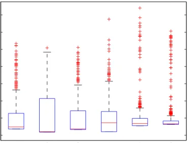
−1 0 1 2 3 4 5 6 1 2 3 4 5 6 Sensor number

Boxplots of data set "Radiant light energy"

Centered and scaled measurements

Figure 3. Boxplots of the six sensors in the “Radiant light energy” data set

4.1

Radiant light energy measurements

The measurements in this data set are from sensors deployed in several office buildings in New York City, as part of Columbia University’s EnHANTs project. The sensors measureirradiance(radiant light energy), and this data set contains values measured during about one year.

Figure 3 shows boxplots of each of the six sensors in this data set, with the measurements centered and scaled as discussed in Section 3. Each boxplot reflects the distribution of the 500 measurements by one sensor, and highlights possible outliers. Each sensor contains 40-60 possible outliers, except for the second sensor which has just one. The Peeling algorithm from Section3.1will select which of these points we will use as outliers in our experiments. Note also that the median of each sensor’s values (except sensor 4) is close to the .25 quantile, indicating that those distributions are skewed towards the smaller values.

More detailed information on the data set can be found in Gorlatova et al.

(2011), or from the CRAWDAD website (Gorlatova et al. (2011)) where the data can be downloaded. For computational reasons, we do not use all the data for the experiments in this paper, but select 500 random measurements from each of the six sensors.

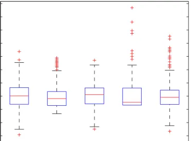
−1 0 1 2 3 4 1 2 3 4 5 6 7 Sensor number

Boxplots of data set "Signal strength"

Centered and scaled measurements

Figure 4. Boxplots of the seven sensors in the “Signal strength” data set

4.2

Signal strength data

This data originates from a WSN deployed in a library building, where sensors measure radio frequency energy level (RSSI) on all 802.15.4 channels in the 2.4 GHz ISM Band. In essence, RSSI is an indication of the power level of a signal received by the antenna on the sensor node. The building has several collocated Wi-Fi networks in normal operation that cause interference, so the WSN is used to monitor the signal strengths on one location in this Wi-Fi network. The WSN consists of 16 sensor nodes (each monitoring a single Wi-Fi channel) of which we used only 7, because the performance of convex hull algorithm in Onion Peeling decreases significantly for dimensions higher than 8 (seeBarber et al. (1996)). Again, we took 500 randomly selected measurements of each node to form this data set.

The boxplots of the sensor values in this data set are shown in Figure4. In contrast to “Radiant light energy” data set, the measurements of the sensors in the “Signal strength” data set contain fewer possible outliers and are more evenly distributed. All possible outliers are positive values, corresponding to a strong incoming Wi-Fi signal.

More details about the data can be found in Noda et al. (2011), or in the CRAWDAD repository (Noda et al.(2012)).

−3 −2 −1 0 1 2 3 4 5 6 7 1 2 3 4 5 Sensor number

Boxplots of data set "Decibel levels"

Centered and scaled measurements

Figure 5. Boxplots of the five sensors in the “Decibel levels” data set

dr-technique Light Signal Decibel

pca 0.3333 0 0.3529

mds 0.9091 0.8750 0.8889

t-_sne 0 0 0

Table 1. F1-score (∈[0,1]) of each combination ofdr-technique and data set

4.3

Decibel levels

This data set consists of five sensors nodes deployed in a kindergarten, one in each room of a single-story building, that are used to monitor the indoor climate. Among other parameters, the nodes measure decibel levels, and report these regularly to a central base station. We took 500 measurements from each sensor on a day in May 2011 and included them in this data set.

Figure 5 shows that most sensors have fairly evenly distributed values, with several outliers on both sides of the median. However, kindergartens tend to be noisy rather than quiet, so most outliers are on the positive side of the median.

dr-technique Light Signal Decibel

pca 0.3302 -0.0149 0.3477

mds 0.9119 0.8801 0.8926

t-_sne -0.0045 -0.0061 -0.0064

Table 2. Matthews Correlation (∈[−1,1]) for each combination ofdr-technique and data set

dr-technique Light Signal Decibel

pca 0.7261 -0.1295 0.6398

mds 1.0509 0.9157 0.8971

t-_sne -0.0404 -0.0244 -0.0226

Table 3. Relative Information Score (∈ [−∞,∞]) for each combination of dr -technique and data set

5

Results and discussion

We apply the experimental setup of Section3 to thedr-techniques of Section

2 and summarize the results in Tables1-3. These tables contain the F1-score, Matthews Correlation, and Relative Information score for each combination of _dr-technique and data set, where a high score implies that the technique preserves outliers well on that data set. The F1-scores in Table 1 show that

mdsachieves the highest scores, with values more than twice as large as those

of _pca on the first and third data set. The lowest possible score on all data sets is by t-_sne: an F1-score of 0. With the Matthews Correlation and Relative Information score in Tables 2 and 3 we see similar results: _mds consequently attains high scores, _pca performs reasonably well on the first and third data set, and t-_snehas overall low scores.

Since we reduce each data set to two dimensions, we can plot the resulting low-dimensional data set and inspect what happens with outliers after applying the three dr-methods. In Figures 6-8 we plot the low-dimensional version of the second data set “Signal strength” (in circles), with outliers in the original high-dimensional data set marked with a triangle. Figure6shows that several of the outliers are mapped to the interior of the reduced data set by_pca. In contrast, the low-dimensional data set created by_mdsshows all high-dimensional outliers close to the boundary. Lastly, t-_snemaps all outliers to the interior of the low-dimensional data set, which illustrates its low scores.

By analysing the objective of the three _dr-techniques, we can explain the ob-served differences in performance. Firstly, _pca is a technique that focuses on preserving variance, so it will only preserve outliers if they happen to be in a direction of high variance. Figure1 from the introduction provides another

illustration of what can happen to an outlier that is in a direction with low variance. The figure corresponds to reducing a two-dimensional data set to one dimension (the line) withpca, and clearly shows how the top-left outlier ends up in the center of the reduced data set.

mds optimizes the squared stress optimization criterion in Eq. (4), which in-cludes the term||xi−xj||M. This term is the distance between two pointsxi

andxj, which is typically very large when one of the points is an outlier. The

criterion uses these distances to the power4, so the outliers have a large effect on the squared stress criterion. Hence, minimizing these distances has a massive positive effect when on this criterion and thus_mdspreserves outliers well. t-_sne optimizes the Kullback-Leibler divergence (8), which attaches high costs to nearby points in high dimensional space (large pij) that are mapped to far

away points in low dimensional space (smallqij). Hence, nearby points in high

dimensional space are kept nearby in low dimensional space. This does not hold for points that are far away in high dimensional space – outliers, which have low pij – as they are mapped to nearby points (with high qij) with very low

costs. So t-snetries to keep nearby points nearby and is therefor more suitable for preserving clusters than for preserving outliers.

Also, t-_snehas some computational complexities. The Kullback-Leibler diver-gence in Eq. (8) is a non-linear function of the low-dimensional pointsyi and

can have several local minimums. Minimizing Eq. (8) is done by choosing a random starting point for theyi, followed by a number of optimization steps

us-ing, e.g., a Gradient Descent approach. The optimization stops when it reaches a (possibly local) minimum, and returns its latest values for theyi. Hence, the

low-dimensional points depend on the starting point chosen for the optimization algorithm, and thus its performance with respect to outlier preservation also de-pend on the starting values of theyi. The last rows of Tables1-3show the score

for one particular starting point, but we repeated the experiments with t-_sne for various starting points. We discovered no correlation between the minimized value of the Kullback-Leibler divergence and the achieved performance score, so the results reported in Tables 1-3 are representative for the performance of t-sne.

From the analysis above we see that from the three selected methods, _mds achieves the highest scores and is best capable of preserving outliers. However, it is not necessarily the best _dr-technique available, since many others exist in literature. In particular, the class of supervised _dr-techniques (_pca, _mds, t-_sne are unsupervised) might provide methods with better performance than

mds. These techniques aim to reduce dimensionality while simultaneously trying

to retain “sufficient information” for a classification task (which, in our case, would be retaining outliers). Hence, they could be applied to the scenario in this paper, and possibly have good performance. Nevertheless, supervised_dr -techniques are not included here, because we assume that the _dr-techniques

−3 −2 −1 0 1 2 3 4 5 −3 −2 −1 0 1 2 3 4

Data set "Signal strength" reduced with PCA.

y_i1

yi2

Reduced data Outliers in high dim

Figure 6. Data set “Decibel levels” after dimensionality reduction withpca(circles). The triangles mark the outliers that were found in the original high-dimensional data set

have no apriori knowledge about the outliers, and thus they are not suitable for this paper. Readers interested in supervised_dr-techniques are referred to, e.g.,

Shyr et al.(2010).

The performance measures in this paper are all based on the elements of the confusion matrix, which do not contain information about whether a point is a ‘large’ or ‘small’ outlier. Hence, with these scores we will not be able to, e.g., find out which outlier has the large affect on a score. This ‘binary’ view of an outlier is, however, important for the scenario in the current paper. Our motivation comes from applications where it is of critical importance to correctly identify an outlier after_dr. If an outlier is no longer an outlier after_dr, then it is useless for the application. Nevertheless, if this ‘binary’ approach can be relaxed from the point of view of the application, other scores might be more appropriate (see, e.g.,Bradley(1997)).

6

Conclusions and recommendations

In this paper we described three well-known Dimensionality Reduction tech-niques (Principal Component Analysis, Multidimensional Scaling, and t-Stochastic Neighbourhood Embedding) and analysed how well they are capable of preserv-ing outliers. Based on three different scores (F1-score, Matthews Correlation,

−4 −2 0 2 4 6 −4 −3 −2 −1 0 1 2 3 4 5

Data set "Signal strength" reduced with MDS.

y_i1

yi2

Reduced data Outliers in high dim

Figure 7. Data set “Decibel levels” after dimensionality reduction withmds(circles). The triangles mark the outliers that were found in the original high-dimensional data set −25 −20 −15 −10 −5 0 5 10 15 20 25 −20 −15 −10 −5 0 5 10 15 20

Data set "Signal strength" reduced with t−SNE.

y_i1

yi2

Reduced data Outliers in high dim

Figure 8. Data set “Decibel levels” after dimensionality reduction with t-sne(circles). The triangles mark the outliers that were found in the original high-dimensional data set

and Relative Information score), and using three real-world data sets, we as-sessed the performance of each method on each data set.

The resulting analysis shows that, among the three describeddr-methods, Mul-tidimensional Scaling is best at preserving outliers. It consequently achieves the highest scores, and performs significantly better than both Principal Compo-nent Analysis and t-Stochastic Neighbourhood Embedding. In the discussion, we explain that this difference in performance is caused by the specific objectives of the techniques: _pcatries to preserve variance,_mdspreserves large distances (i.e. outliers), and t-_snepreserves clusters. In general, we recommend that the dimensionality reduction technique is chosen with the intended application in mind. For outlier detection_mds is a good choice, for preserving variance_pca is the best choice, and for preserving clusters t-_sneis a good choice.

Future research includes investigating specific types of Dimensionality Reduc-tion (e.g. supervised _dr-methods, real-time _dr-methods), and how they are affected by outliers.

Acknowledgements

This work is based on a report by Onderwater (2010) of an internship at the Fraud Detection Expertise Center at VU University Amsterdam. The current paper is part of the project RRR (Realisation ofReliable and SecureResidential Sensor Platforms) of the Dutch programIOP Generieke Communicatie, number IGC1020, supported by theSubsidieregeling Sterktes in Innovatie. We would like to thank Arnoud den Boer (CWI, VU University) for his feedback on the drafts of this document, and Munisense B.V. (Leiden, The Netherlands) for providing one of the data sets.

References

Agyemang, M., K. Barker, and R. Alhajj (2006). A comprehensive survey of nu-meric and symbolic outlier mining techniques. Intelligent Data Analysis 10(6), 521–538.

Barber, C. B., D. P. Dobkin, and H. Huhdanpaa (1996). The quickhull algo-rithm for convex hulls. ACM Transactions on Mathematical Software 22(4), 469–483.

Becker, R. A., C. Volinsky, and A. R. Wilks (2010). Fraud detection in telecom-munications: History and lessons learned. Technometrics 52(1), 20–33.

Bradley, A. P. (1997). The use of the area under the ROC curve in the evaluation of machine learning algorithms. Pattern recognition 30(7), 1145–1159. Cao, H., D. H. Hu, D. Shen, D. Jiang, J.-T. Sun, E. Chen, and Q. Yang (2009).

Context-aware query classification. In Proceedings of the 32nd international ACM SIGIR conference on Research and development in information retrieval, pp. 3–10.

Carreira-Perpinán, M. A. (1997). A review of dimension reduction tech-niques. Department of Computer Science. University of Sheffield. Tech. Rep. CS-96-09, 1–69.

Chakrabarti, K. and S. Mehrotra (2000). Local dimensionality reduction: A new approach to indexing high dimensional spaces. In Proceedings ofthe 26th VLDB Conference, pp. 89–100.

Dai, J. J., L. Lieu, and D. Rocke (2006). Dimension reduction for classification with gene expression microarray data. Statistical applications in genetics and molecular biology 5(1).

Escalante, H. J. (2005). A comparison of outlier detection algorithms for ma-chine learning. In CIC-2005 Congreso Internacional en Computacion. Fodor, I. (2002). A survey of dimension reduction techniques. Technical Report

UCRL-ID-148494, Lawrence Livermore National Laboratory.

Garg, V. K. and M. N. Murty (2009). Feature subspace SVMs (FS-SVMs) for high dimensional handwritten digit recognition. International Journal of Data Mining, Modelling and Management 1(4), 411.

Ghodsi, A. (2006). Lecture notes of lecture 9 of the course "Data visualization" (STAT 442). Technical report, University of Waterloo.

Gogoi, P., D. Bhattacharyya, B. Borah, and J. K. Kalita (2011). A survey of outlier detection methods in network anomaly identification. Comput. J. 54(4), 570–588.

Gorlatova, M., A. Wallwater, and G. Zussman (2011). Networking low-power energy harvesting devices: Measurements and algorithms. In INFOCOM, 2011 Proceedings IEEE, pp. 1602 –1610.

Gorlatova, M., M. Zapas, E. Xu, M. Bahlke, I. Kymissis, and G. Zussman (2011). CRAWDAD data set columbia/enhants (v. 2011-04-07). Published: Downloaded from http://crawdad.cs.dartmouth.edu/columbia/enhants. Gupta, R. and R. Kapoor (2012). Comparison of graph–based methods for

non–linear dimensionality reduction. International Journal of Signal and Imaging Systems Engineering 5(2), 101–109.

Hahn, L. W., M. D. Ritchie, and J. H. Moore (2003). Multifactor dimen-sionality reduction software for detecting gene–gene and gene–environment interactions. Bioinformatics 19(3), 376–382.

Härdle, W. K. and L. Simar (2012). Applied Multivariate Statistical Analysis. Springer.

Harmeling, S., G. Dornhege, D. Tax, F. Meinecke, and K.-R. Müller (2006). From outliers to prototypes: Ordering data. Neurocomputing 69(13–15), 1608–1618.

Hinton, G. and S. Roweis (2002). Stochastic neighbor embedding. In Advances in Neural Information Processing Systems 15, pp. 833–840. MIT Press. Hodge, V. and J. Austin (2004). A survey of outlier detection methodologies.

Artif. Intell. Rev. 22(2), 85–126.

Johnson, R. and D. Wichern (2002). Applied Multivariate Statistical Analysis. Prentice Hall.

Kandaswamy, K. K., G. Pugalenthi, K.-U. Kalies, E. Hartmann, and T. Mar-tinetz (2012). EcmPred: prediction of extracellular matrix proteins based on random forest with maximum relevance minimum redundancy feature selec-tion. Journal of theoretical biology.

Kline, D. M. and C. S. Galbraith (2009). Performance analysis of the bayesian data reduction algorithm. International Journal of Data Mining, Modelling and Management 1(3), 223.

Kohonen, T. (2001). Self-organizing maps (3rd ed.), Volume 30. Springer. Kononenko, I. and I. Bratko (1991). Information-based evaluation criterion for

classifier’s performance. Machine Learning 6(1), 67–80.

Lattin, J., D. Carroll, and P. Green (2003). Analyzing Multivariate Data. Thom-son Learning.

Li, K.-C. (1992). On principal hessian directions for data visualization and dimension reduction: Another application of stein’s lemma. Journal of the American Statistical Association 87(420), 1025–1039.

Maalouf, M. and T. B. Trafalis (2011). Rare events and imbalanced datasets: an overview. International Journal of Data Mining, Modelling and Management 3(4), 375.

Mahalanobis, P. C. (1936). On the generalized distance in statistics. In Proceedings of the national institute of sciences of India, Volume 2, pp. 49–55. Martins, B., I. Anastácio, and P. Calado (2010). A machine learning approach for resolving place references in text. In M. Painho, M. Y. Santos, and H. Pundt (Eds.), Geospatial Thinking, Number 0 in Lecture Notes in Geoin-formation and Cartography, pp. 221–236. Springer Berlin Heidelberg.

Matthews, B. (1975). Comparison of the predicted and observed secondary structure of t4 phage lysozyme. Biochimica et Biophysica Acta (BBA) -Protein Structure 405(2), 442–451.

Mondal, S., R. Bhavna, R. Mohan Babu, and S. Ramakumar (2006). Pseudo amino acid composition and multi-class support vector machines approach for conotoxin superfamily classification. Journal of Theoretical Biology 243(2), 252–260.

Muñoz, A. and J. Muruzábal (1998). Self-organizing maps for outlier detection. Neurocomputing 18(1–3), 33–60.

Nguyen, H. V., V. Gopalkrishnan, H. Liu, H. Motoda, R. Setiono, and Z. Zhao (2010). Feature extraction for outlier detection in highdimensional spaces. In The 4th Workshop on Feature Selection in Data Mining.

Noda, C., S. Prabh, M. Alves, C. A. Boano, and T. Voigt (2011). Quantifying the channel quality for interference-aware wireless sensor networks. SIGBED Rev. 8(4), 43–48.

Noda, C., S. Prabh, M. Alves, T. Voigt, and C. A. Boano (2012). CRAWDAD data set cister/rssi (v. 2012-05-17). Published: Downloaded from http://crawdad.cs.dartmouth.edu/cister/rssi.

Onderwater, M. (2010). Detecting unusual user profiles with outlier detection techniques. M.Sc. thesis, http://tinyurl.com/vu-thesis-onderwater.

Pearson, K. (1901). On lines and planes of closest fit to systems of points in space. Philosophical Magazine Series 6 2(11), 559–572.

Phua, C., V. Lee, K. Smith, and R. Gayle (2005). A comprehensive survey of data mining-based fraud detection research. Technical report, Monash University.

Powers, D. M. W. (2011). Evaluation: From precision, recall and f-measure to ROC., informedness, markedness & correlation. Journal of Machine Learning Technologies 2(1), 37–63.

Ravi, V. and C. Pramodh (2010). Non-linear principal component analysis-based hybrid classifiers: an application to bankruptcy prediction in banks. International Journal of Information and Decision Sciences 2(1), 50.

Sha, F. and F. Pereira (2003). Shallow parsing with conditional random fields. In Proceedings of the 2003 Conference of the North American Chapter of the Association for Computational Linguistics on Human Language Technology-Volume 1, pp. 134–141.

Shannon, C. E. (1948). A mathematical theory of communication. Bell system technical journal 27.

Shen, H.-B. and K.-C. Chou (2007). Using ensemble classifier to identify mem-brane protein types. Amino Acids 32(4), 483–488.

Shyr, A., R. Urtasun, and M. I. Jordan (2010). Sufficient dimension reduction for visual sequence classification. In 2010 IEEE Conference on Computer Vision and Pattern Recognition (CVPR), pp. 3610–3617.

Tabachnick, B. G. and L. S. Fidell (2001). Using multivariate statistics. Allyn and Bacon.

Tenenbaum, J. B., V. d. Silva, and J. C. Langford (2000). A global geometric framework for nonlinear dimensionality reduction. Science 290(5500), 2319– 2323.

Tsai, F. S. (2012). Dimensionality reduction framework for blog mining and visualisation. International Journal of Data Mining, Modelling and Management 4(3), 267–285.

UmaMaheswari, P. and M. Rajaram (2009). Principal component analysis-based frequent pattern evaluation on the object-relational data model of a cricket match database. International Journal of Data Analysis Techniques and Strategies 1(4), 364.

Valstar, M. F., B. Jiang, M. Mehu, M. Pantic, and K. Scherer (2011). The first facial expression recognition and analysis challenge. In Automatic Face & Gesture Recognition and Workshops (FG 2011), 2011 IEEE International Conference on, pp. 921–926.

Van der Maaten, L. (2009). Dimensionality reduction toolbox.

Van der Maaten, L. and G. Hinton (2008). Visualizing data using t-SNE. Journal of Machine Learning Research 9, 2579–2605.

Van der Maaten, L., E. Postma, and J. Van den Herik (2009). Dimensionality reduction: A comparative review. Technical Report 2009-005, Tilburg centre for Creative Computing, Tilburg university.

Yoon, S. (2003). Singular Value Decomposition & Application.

Zhang, Y., N. Meratnia, and P. Havinga (2010). Outlier detection techniques for wireless sensor networks: A survey. IEEE Communications Surveys & Tutorials 12(2), 159–170.

Zhang, Y., N. Meratnia, and P. J. M. Havinga (2007). A taxonomy framework for unsupervised outlier detection techniques for multi-type data sets. Number TR-CTIT-07-79. Enschede: Centre for Telematics and Information Technol-ogy, University of Twente.