Degree project in Computer Science
OSKAR ARVIDSSON
OSKAR ARVIDSSON
Master’s Thesis at CSC Supervisor: Mikael Goldmann
Code obfuscation is a technique used to make soft-ware more difficult to read and reverse engineer. It is used in the industry to protect proprietary algo-rithms and to protect the software from unintended use. The current state of the art solutions in the in-dustry depend on specific platform targets. In this report we look at code obfuscation from a platform independent point of view. The result is a survey of code obfuscation methods that can be used together to perform platform independent code obfuscation. We also analyze some of these methods in more de-tail and provide insights regarding their potency (dif-ficulty to deobfuscate manually), resilience (dif(dif-ficulty to deobfuscate automatically), stealth (difficulty to distinguish from normal code) and ease of integra-tion (how easily the method can be integrated and used in a toolchain).
Referat
Plattformsoberoende kodobfuskering
Kodobfuskering är ett verktyg för att göra mjukvara svårare att läsa, förstå och bakåtkompilera. Det an-vänds inom industrin för att skydda proprietära algo-ritmer samt för att skydda program och tjänster från att missbrukas. De lösningar som finns att tillgå idag är dock ofta beroende av en eller flera specifika platt-formar. I den här rapporten undersöker vi möjlighe-ten att göra plattformsoberoende obfuskering. Resul-tatet är en undersökning av vilka obfuskeringsmeto-der som finns tillgängliga, samt en djupare studie av några av dessa. Den djupare studien ger, för var och en av de studerade metoderna, insikter om hur svåra de är att deobfuskera för hand, hur svåra de är att deobfuskera automatiskt, hur pass svårt det är att skilja den obfuskerade koden från den oobfuskerade, samt hur lätt det är att implementera och integrera dem i en kompileringskedja.
The work that this report is based on was in part carried out together with Oskar Werkelin Ahlin. I would like to thank him both for his support during the study, implementation and evaluation of different code obfuscation techniques, and for his encourage-ment during the whole process. Next I would like to thank my supervisors Mikael Goldmann and Henrik Österdahl. They have given me excellent feedback during the course of the project. Without their ef-fort this report would not have become what it is. Finally I want to thank Johan Håstad for his advice and feedback during the final work on the report.
1 Introduction 1 1.1 Motivation . . . 1 1.2 Purpose . . . 2 1.3 Outline . . . 3 2 Background 4 2.1 Terminology . . . 4 2.2 Code obfuscation . . . 4 2.2.1 History . . . 4 2.2.2 Definition . . . 5
2.2.3 State of the art . . . 5
2.3 Compiler technology . . . 6 2.3.1 Front end . . . 7 2.3.2 Back end . . . 9 2.3.3 Common compilers . . . 11 2.4 Reverse engineering . . . 13 2.4.1 Static analysis . . . 13 2.4.2 Dynamic analysis . . . 14 2.4.3 Program slicing . . . 15
2.5 Code obfuscation methods . . . 15
2.5.1 Layout obfuscation methods . . . 16
2.5.2 Data obfuscation methods . . . 16
2.5.3 Control flow obfuscation methods . . . 19
2.6 Obfuscation quality . . . 25 2.6.1 Potency . . . 25 2.6.2 Resilience . . . 27 2.6.3 Execution cost . . . 27 2.6.4 Stealth . . . 28 2.6.5 Ease of integration . . . 28 3 Method 29
3.2.2 Function transformations . . . 31 3.2.3 Exception exploitations . . . 34 3.2.4 Value encoding . . . 35 3.3 Evaluation . . . 38 4 Implementation 41 4.1 Tools . . . 41 4.2 Obfuscator . . . 42 4.2.1 Obfuscation methods . . . 42 4.2.2 Constant pool . . . 42 4.2.3 Opaque predicates . . . 42 4.2.4 Toolchain integration . . . 43 4.3 Testing . . . 44 4.4 Analysis . . . 44 5 Results 45 5.1 Potency and cost . . . 45
5.1.1 Value encoding . . . 46
5.1.2 Function pointer transformations . . . 47
5.1.3 Function transformations . . . 48
5.1.4 Exception exploitation . . . 48
5.1.5 All obfuscations . . . 49
5.2 Resilience . . . 50
5.2.1 Value encoding . . . 50
5.2.2 Function pointer transformations . . . 50
5.2.3 Function transformations . . . 51
5.2.4 Exception exploitation . . . 52
5.3 Ease of integration . . . 52
5.3.1 Value encoding . . . 52
5.3.2 Function pointer transformations . . . 52
5.3.3 Function transformations . . . 53
5.3.4 Exception exploitations . . . 53
5.4 Stealth . . . 53
5.4.1 Value encoding . . . 53
5.4.2 Function pointer transformations . . . 54
5.4.3 Function transformations . . . 54
6.1.2 Subjective Thoughts . . . 57 6.2 Future work . . . 58
Introduction
There are many different techniques for a company to protect its intellectual ideas against competitors and their services against unintended use. This report studies one such technique. Code obfuscation is a collection of methods that can be used to protect software against reverse engineering. Reverse engineering is a process that transforms the output of another process into the input of said process in part or completely. An example of this is to reconstruct the source code from a compiled program.
The application of code obfuscation does not guarantee that a program cannot be reverse engineered, but its purpose is to make the process of reverse engineering prohibitively expensive. Combined with other techniques for pro-tecting software against third party tampering, code obfuscation can serve as an important tool for software protection in the industry.
1.1
Motivation
Consider the process of distributing software from one party to another. One party acts as distributor (the company) and the other party acts as user of the software. According to tradition, we will call the first party Alice and the second party Bob. Alice wants to distribute her software service in a way so that Bob cannot easily reverse engineer it and reveal the secrets of her code. The secrets can be anything from encryption keys to algorithms. It is important that Bob can run the software efficiently in the way it was intended to, otherwise Bob might choose to use another service instead.
As of today, there are many ways to approach this problem. Alice can choose to distribute the software as an online service, keeping the important parts of the code away from Bob’s computer. This could be done with the
requires that Bob has Internet access while running the program, and it also might require Alice to solve the problem of dealing with high server load.
Another solution for Alice could be to use hardware support to secure the software. A specific hardware device would be required for using the service. This would require an attacker to analyze how such a device works. Even though such an approach seems secure, it would be tedious to distribute such a program due to the requirement of a physical hardware device. Furthermore, if an attacker is able to disable or bypass the device, the system would still be open for attacks.
Code obfuscation aims to hide Alice’s secrets through obscuring the code from third party inspection. Code obfuscation does not obstruct Bob from running the program in the way he usually does. In fact it preserves its functionality, albeit at a slight decrease in performance. Bob may try to reverse engineer the code, but the obfuscations will make that process more difficult, time consuming and bothersome.
Let us consider the following scenario: Alice wants to distribute her soft-ware to as many customers as possible, so she is planning to do it for desktops as well as mobile clients. Most of the customers use standard operating sys-tems such as Microsoft Windows or Apple Mac OS X on a personal computer. But there are also people who would like to use her software on their smart phones, tablets, etc. Recently she has also been approached by companies who want to embed her application into their hardware. She wants to protect her software on all these platforms.
Over the years, tools have appeared that can obfuscate code for specific platforms, but since they depend on specific platforms, they need to be re-vamped as new platforms appear. Each of them implements different obfus-cation methods. The methods have different characteristics regarding how difficult they are to implement, the cost of using them and how easy they are to remove by an attacker. We are interested in looking at a subset of these methods that are independent of the target platform.
1.2
Purpose
The long-standing problem of protecting software secrets against a potentially malicious third party today needs to be addressed for multiple platforms, rang-ing from common personal computers to integrated systems with specially designed operating systems. Even more so, with new platforms emerging con-stantly, platform independent code obfuscation could be a potent, economic and practical protection against a malicious third party.
reason about how they can be used independently of target platform. The most interesting methods are evaluated and analyzed according to common practice in the field. We also analyze and evaluate combinations of them.
Finally, the aim of the report is to present some recommendations on how a system for target platform independent code obfuscation could be built.
1.3
Outline
Chapter 2 serves as an introduction to the current research in the field, both in terms of what methods for code obfuscation exist and how they can be evaluated and analyzed. In chapter 3 we lay out and motivate the selection of the approach that was used for evaluating the chosen obfuscations. We also present and motivate our choice of analysis methods, which have been derived from current research in the subject area. Chapter 4 discuss in more detail how the obfuscation methods were implemented. In chapter 5 we present the results of the analysis. Finally we present our conclusions in chapter 6, where we also discuss future work and what could have been done differently.
Background
In this chapter we describe important theory and concepts that can aid in understanding the following sections.
2.1
Terminology
This section define terms that are used throughout the report.
Obfuscator A program that obfuscates an input program, emitting an obfus-cated output program with equivalent semantics compared to the input.
Toolchain A set of tools that are used to create a software product. Tools are usually chained in a specific way. A simple example of a toolchain is a source code editor and a compiler used to compile the source code.
CPU Central processing unit, mostly referred to as the computer processor.
2.2
Code obfuscation
Code obfuscation is a collective term for techniques that make code more difficult to read and reverse engineer.
2.2.1
History
Techniques for code obfuscation were first formalized by Collberg et al. 1997 [4]. Although code obfuscation had been used prior to this date, academic research in the area had been sparse until then. At first there were hopes that obfuscation could be used as a black box providing encryption similar to
could exist in this sense. The results found by Barak et al. more or less halted the academic research in the area of code obfuscation for many years, although companies kept using it practically. Little academic progress was made until 2004 when Lynn et al. [21] showed the first positive results about obfuscation. They showed how obfuscation can be applied on access control graphs, and observed that a similar approach probably could be used for obfuscating finite automata or regular expressions.
Code obfuscation has been used in one way or another in the industry for a long time. Lately, its usefulness in malware creation has been discovered [26], making it more difficult to do code analysis on viruses thus making it more difficult for anti-virus programs to detect malicious software. Much of the academic research during the last years has thus focused on deobfuscating obfuscated software in order to protect users from malware.
2.2.2
Definition
In order to reason about the correctness of an obfuscation method, we first need to define formally what an obfuscation is. Collberg et al. [4] proposed the following definition:
Let P → P0 be a transformation of a source program P into a target program P0. P →P0 is an obfuscating transformation, if P and P0 have the same observable behavior. More precisely, in order for P → P0 to be a legal obfuscating transformation the following must hold:
• If P fails to terminate or terminates with an error condition, then P0
may or may not terminate.
• Otherwise, P0 must terminate and produce the same output as P. Collberg et al. defined the observable behavior to be the behavior of the program “as experienced by the user”. What this means is that P0 may have side-effects thatP does not have, but they should be acceptable and go unno-ticed by the user. Collberg et al. further elaborates about the memory usage and speed difference between P and P0 and states that such differences are valid side effects.
2.2.3
State of the art
There are a few proprietary obfuscation tools available for usage. Most of them are designed for a specific platform in order to allow for increased
ef-Themida
Themida is a proprietary software protection system for Windows developed by Oreans Technologies. It works on a binary level, obfuscating compiled Windows x86 binaries. Among its notable features it includes anti-debugging, anti-memory dump (a snapshot of the working memory of a process at a specific time) and binary integrity checks (ensures that the program can only run if not modified). It also includes functionality for hiding code inside a virtual machine which is obfuscated in itself, increasing the obfuscation level significantly. As Themida not only obfuscates code, it is much more than an obfuscation tool, targeting to protect a program from reverse engineering altogether. [28]
Morpher
Morpher is a compiler driven obfuscation tool developed by MTC Group LTD. Morpher has support for a large number of obfuscation methods, and supports using them in arbritary combinations. It makes use of its tight coupling with the languages’ compilers to be able to apply more sophisticated transforms which require more information about the source code.
It has support for standard C/C++, and limited support for Fortran95 and Ada. Supported architectures are x86, PowerPC and ARM among others. The obfuscator tool is built on llvm-gcc (see Section 2.3.3). Among its notable features Morpher has support for protecting constant values (e.g. values are stored encrypted, and decrypted only upon use) and function transformations. [20]
Diablo
Diablo is an open source infrastructure for rewriting binaries. Development is currently stalled, but some obfuscation methods have been implemented previously. One of the features is control flow graph flattening. Support exists for x86 and ARM. [14]
2.3
Compiler technology
A compiler is by definition a computer program that transforms source code into another form, e.g. native code. The process of compiling source code can usually be divided into a number of steps, which are briefly described in this section. A standard compiler can be divided into two main parts, namely the front end and the back end. There are no exact rules for how a compiler
should be written; the description below rather describes one approach. This section is based onEngineering a Compiler by Cooper and Torczon [6].
2.3.1
Front end
Part of the compiler front end is lexical analysis, parsing and semantic analysis. The lexical analysis and parsing are often jointly referred to as syntactical analysis.
Lexical analysis
Lexical analysis is the process of transforming the flow of characters of the in-put source code into a sequence of tokens describing the program. Conversely, a token describes a sequence of characters in the source code. Examples of tokens that can be useful for a C compiler front end are IF, ELSE, FOR,
RETURNandAND, but a C string literal such as “a string” can also make up a token. The purpose of the lexical analysis is primarily to make the code easier to process for the parser. Listing 2.1 shows a program and Listing 2.2 shows a possible result from an imaginary lexer when fed with the program in Listing 2.1. Note that each token in the lexical analysis often is associated with the sequence of characters it represents in the source input. This infor-mation is needed to e.g. extract the contents of a string or the name of an identifier.
1 i n t main(i n t argc, const char ∗∗argv) { 2 p r i n t f("%d %s \n ", argc−1, argv[ 0 ] ) ;
3 return 0 ;
4 }
Listing 2.1. A simple example program.
1 INT ID PAR_BEGIN INT ID COMMA CONST CHAR STAR STAR ID PAR_END
CURLY_BEGIN ID PAR_BEGIN STRING COMMA ID MINUS NUM COMMA ID SQUARE_BEGIN NUM SQUARE_END PAR_END SEMICOLON RETURN NUM SEMICOLON CURLY_END
Listing 2.2. Example of what the lexical analysis of the program in Listing
Parsing
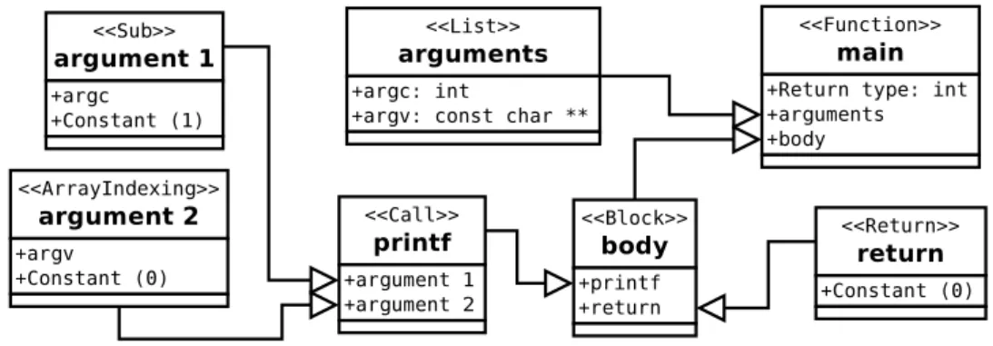
Input to the parser is the output from the lexical analysis. Output from the parser is an abstract syntax tree (AST). Nodes in the AST are abstract concepts of the source language. A node may have static attributes, such as the name of the function in a function declaration, and child nodes, such as the arguments in a function call. The parser ensures that the input is part of the source language grammar, and emits a syntactic error if this is not the case. Figure 2.1 shows the output from an imaginary parser fed with the output from Listing 2.2.
Figure 2.1. Example of an AST that could be generated from the program
in Listing 2.1.
Semantic Analysis
Input to the semantic analysis is an AST. The purpose of the semantic analysis is solely to ensure that the program is semantically correct. Common errors that the semantic analysis should detect are references to non-existing iden-tifiers (names of variables, functions and similar constructs), type errors, etc. To help in the process, the compiler creates a symbol table, which contains information about the visible identifiers in different scopes within the code. Apart from being used as a means to do semantic analysis of the code, the symbol table can be output for further use by later phases in the compiler.
Intermediate code generation
A compiler may support multiple input languages and multiple output for-mats. Common input languages are for example C and C++, and it is not uncommon that a user of a compiler will want to target two or more
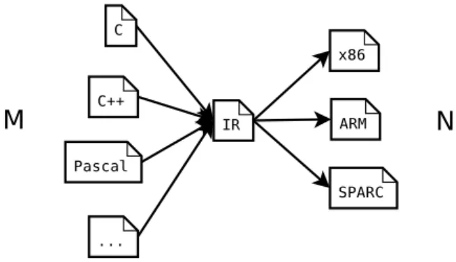
com-differences such as operating system here). One way to support this is to write one compiler for compiling C code to x86, another for C++ to x86 and similarly one more compiler able to compile source of each input language to ARM native code. In the general case this would require M ×N compilers, where M is the number of input languages and N is the number of output formats.
While specialized compilers may sometimes be useful, a more general-purpose approach is to write one front end for each input language that compiles the code to a common intermediate language, and one back end for each output format. Figure 2.2 illustrates this process. The intermediate representation needs to be complex enough to cover all constructs in all input languages. In contrast to the specialized approach, with M ×N compilers, this approach only requiresM compiler front ends and N compiler back ends. Furthermore, the most difficult and advanced part of a compiler is analysis and optimizations. Parts of the analysis and optimizations can be done on the intermediate code, reducing the amount of work required to write a back end for a new output format.
Figure 2.2. An illustration of the purpose of the intermediate code.
It should be noted that almost every compiler uses its own language and conventions for intermediate code (IR). One common property shared by many of these languages is single static assignment (SSA). In SSA each variable is assigned exactly once, i.e. it is not allowed to write to a distinct variable multiple times. A simple example of IR code on the SSA form can be seen in Figure 2.3.
2.3.2
Back end
gen-x←0 y←5 y←x∗y x←x∗y x1 ←0 y1 ←5 y2 ←x1∗y1 x2 ←x1∗y2
Figure 2.3. A sample program to the left and its SSA transformation to the
right.
which contains compiled code and some associated information such as ex-ported symbols, for the target machine. A file containing object code is called an object file. Finally a linker phase is needed in order to combine multiple object files into one executable file.
Analysis and optimizations
One of the most important properties of a compiler is the quality of its op-timizations. In order to do optimizations on the code, the compiler needs to analyze the code. The analysis done by a compiler has much in common with static analysis that an attacker can perform as described later.
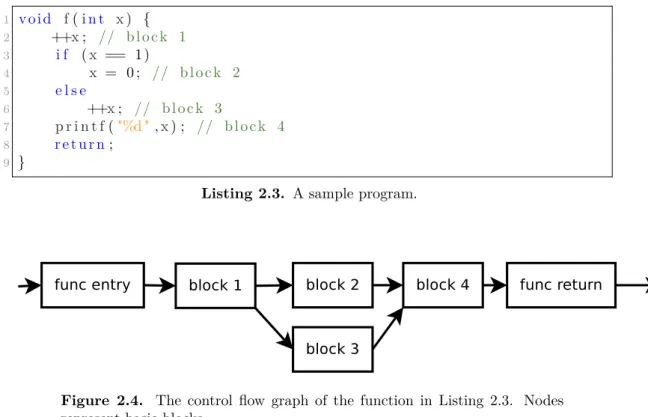
Input to the optimization phase is intermediate code. The intermediate code is parsed into one or more control flow graphs (CFG) which are similar to an AST, but on a much more detailed level. The nodes in the CFG consist of basic blocks. One basic block is a small piece of code that fulfills certain requirements. Most importantly, only the last instruction in a basic block can be a branch instruction. Each branch instruction corresponds to a directed edge in the CFG from one basic block to one or more basic blocks. In the most basic case, each function in the source code will translate to one CFG. A CFG may have one or more exit nodes, corresponding to different return points in a function. A CFG normally has one entry point, corresponding to the start of the function it models. Note that a CFG may also be used to model things apart from functions such as whole programs. Figure 2.4 shows a control flow graph based on the sample code in listing 2.3.
The purpose of control flow graphs is to simplify the process of performing analysis and optimizations. The control flow graphs can also be used for optimization purposes itself. For example, basic blocks with no incoming edges can be discarded as they contain unreachable code.
1 void f(i n t x) { 2 ++x; // block 1 3 i f (x == 1) 4 x = 0 ; // block 2 5 e l s e 6 ++x; // block 3 7 p r i n t f("%d " ,x) ; // block 4 8 return; 9 }
Listing 2.3. A sample program.
Figure 2.4. The control flow graph of the function in Listing 2.3. Nodes
represent basic blocks.
Code generation
Input to the code generation is intermediate code. The code generation phase of the compiler is responsible for instruction selection and register allocation. Instruction selection transforms the instructions of the intermediate code to instructions in the target’s native code such that the semantics of the program is preserved. Register allocation is the process of assigning processor registers efficiently to the variables that need to be represented in the program. When required, the register allocation will spill registers to the stack. Note that instruction selection as well as register allocation is subject to optimizations as well. Output of the code generation phase is native code for the target platform.
2.3.3
Common compilers
GNU Compiler Collection
The GNU Compiler Collection (GCC) is an open-source compiler. It is pro-duced by the GNU project, a free software and mass collaboration project. It has been adopted to be the standard compiler by most Unix-like operating systems, but support exists for Windows as well. GCC uses an intermedi-ate representation that is called GIMPLE. GIMPLE comes in many forms, of which one is SSA based.
GCC is widely used not only in free software projects, but also in commer-cial and proprietary software development. [11]
Low Level Virtual Machine
Low Level Virtual Machine (LLVM) is an open source compiler infrastructure which originally was a research project at the University of Illinois. LLVM is commonly used together with Clang which is a compiler front end with support for C/C++/Objective-C. In this configuration, LLVM acts as the compiler back end. There is also a GCC compatible front end for LLVM called llvm-gcc. This front end intends to be a drop in replacement for GCC on supported platforms, while using the LLVM back end.
One of the main features of LLVM is that it is modular, making it relatively easy to extend. In particular the LLVM documentation covers writing modules that analyse or transform the code. Many of the optimizations done by LLVM are implemented as modules. This architecture stands in contrast to other compilers, where transformation code needs to be built statically into the compiler. Another feature of LLVM is the LLVM IR. LLVM IR is in SSA form, and the same IR can be used as input to all LLVM tools, such as the optimizer, the code generator and interpreter. It can also easily be edited manually without any tools other than a text editor.
LLVM is available for multiple processor architectures, and is able to pro-duce code for x86, x86-64 and ARM as of today. Support for other architec-tures can be added with modules just as with optimization passes. [19]
Microsoft Visual Studio Compiler
The Microsoft Visual Studio Compiler, which is distributed as part of Mi-crosoft Visual Studio is the de facto compiler for Windows programs – al-though many other compilers exist. The Microsoft Visual Studio Compiler is proprietary, and can not be extended with third party code transformation modules. [7]
2.4
Reverse engineering
In this section, different reverse engineering techniques are explained and dis-cussed. We do not go into great depth, since this is not the topic of the report. It is necessary to have a brief understanding of some standard reverse engi-neering techniques in order to understand the benefits of certain obfuscation techniques.
Analysis methods are divided into two main types, namely static and dy-namic analysis.
2.4.1
Static analysis
Static analysis refers to analysis that is carried out without executing a pro-gram. The analysis is carried out on source code describing the propro-gram. Generally the original source of a program is not available for static analy-sis, but only an executable without debugging symbols. Thus static analysis depends on a correct transform from the executable code to a source code representation of the program. This transformation is normally done with a disassembler. Disassembly is not an exact process. In fact, disassembly in general is known to be reducible to the halting problem, thus unsolvable. This needs to be noted when working with static disassembly. Although the static analysis may be correct for the disassembly at hand, the disassembly in itself need not be correct thus invalidating the static analysis. [25]
Data-flow analysis
Data-flow analysis is a technique for determining the set of possible values for variables in certain points of a computer program. For each basic block, we define an entry state sentry and an exit state sexit. By state, we mean
information about the program, e.g. relationships between variables. Define a transfer function f such that f(sentry) = sexit. We also know that sentry
depends on the combined exit states of predecessors of s in the control flow graph. Using this, we get the pair of equations for each node:
sentry =∪s0∈Ss0exit
sexit =f(sentry)
whereS is the set of predecessors tos. By solving these equations, we can determine certain properties about the data flow in each node. [6]
Code cloning
In a program, the same node can often be reached through different execution paths. As the information propagated by data-flow analysis will be more complex for the node in this case, a technique called code cloning is commonly used. Code cloning aims to duplicate nodes so that each node is reachable through exactly one path of nodes. For example, if blockC is reachable either through blockB or blockA, C is split into two blocks CA and CB. This way,
each block will have exactly one predecessor, making the control flow graph larger, but also more simple. [29]
Path feasibility analysis
Path feasibility analysis finds a subset of the dummy edges introduced by control flow obfuscation, and concludes that they are unfeasible, giving the reverse engineer a more simple control flow graph.
Assume that we have an arbitrary acyclic program execution path P, and ¯
x, the set of live variables (variables in use) at entry to P. We want to con-struct a constraintCP such that (∃¯x)CP is unsatisfiable only ifP is unfeasible.
Having constructedCP, we check if it is satisfiable. If it is not, we know that
P is unfeasible.
The condition CP can be constructed using a simple set of rules that
de-pend on the operations performed along the execution path, as explained by Udupa [29].
2.4.2
Dynamic analysis
Dynamic analysis is carried out during program execution. The software is executed on a real or a virtual processor. As opposed to static analysis, which should always give the same result for a specific input, the result of dynamic analysis is highly dependant on how the program is executed. Therefore, it is important to explore a sufficient amount of different program executions to create interesting program behaviour. Techniques such as code coverage can be used to ensure that a sufficient portion of the program’s set of possible execution paths has been explored. During the run, various data can be collected. Examples of such data can be snapshots of the state of the program at different locations in the code, and the control flow graph as traversed when executing the program. [29]
2.4.3
Program slicing
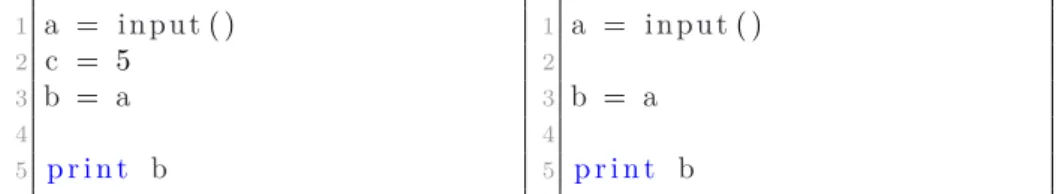
Program slicing is an important technique that can be used both for static and dynamic analysis. A program is sliced according to some slicing criterion, and then all parts that are not affected by the parts of interest are filtered out. This makes the debugging process easier, for example if we want to know why a specific value is incorrect at a specific point in the program, the variable would be selected and slicing would filter out all parts of code that do not affect the variable at hand, directly or indirectly.
1 a = input( ) 2 c = 5 3 b = a 4 5 p r i n t b 1 a = input( ) 2 3 b = a 4 5 p r i n t b
Figure 2.5. A sample program to the left and to the right the result of
program slicing on the last statement.
Consider for example the code in Figure 2.5. Assume that the statement
print b made the program output an unexpected statement. We would slice the program according to this statement, and the slicer would filter out all values that are independent of it. Looking at the example above, slicing on the variable a would filter out the statement c = 5 as it does not affect the variable a in any way. [16]
2.5
Code obfuscation methods
The methods that can be used to obscure source code can be divided into three categories; layout obfuscations, data obfuscations and control flow ob-fuscations. Layout obfuscation only deals with the syntactic elements of the source code, i.e. how the source code is formatted and encoded. Data obfus-cations obscure variables, classes and other data. Control flow obfusobfus-cations change the control flow of the program such that its pattern is less obvious to spot while analyzing the program flow. This section is largely based on the work by Collberg et al. [4] and Drape [9]. Note that we put the emphasis on describing the concept of the methods, rather than elaborate on when they can be used without changing the semantics.
2.5.1
Layout obfuscation methods
Layout obfuscations have in common that they only change syntactic elements in the code, i.e. they change the appearance of the code while leaving the real structure intact. Normally this type of transformation is unnecessary as the compiler already removes this structure from the code. However if the code is to be redistributed as is, i.e. in source code, methods of this type can be used to remove some of the human readable information. For source distribution, these transformations actually can provide an important means of protection as variable names and other syntactic sugar provide a human reader with context for better comprehension of the code even if it have been obfuscated by other means.
Scrambling identifiers
Scrambling identifiers is the process of renaming identifiers such as variable and function names. It aims to change these identifiers to names which do not explain what they are used for, or to names that are illogical to what they are used for. Figure 2.6 shows an example of this.
int confirmLogin() ... int apples() ...
Figure 2.6. An example of how identifier names can be rewritten.
With most compiled languages, this information is not preserved by the compiler – if the identifiers are not explicitly or implicitly exported in any way such as through the use of debugging information. Removing this type of information from native executables is called stripping.
Remove comments
Comments often contain high level information such as why the code works in a specific way, and what the purpose of the code is. This informatin can be removed without any semantic changes. Similarily to the process of scrambling identifiers, this process is normally only useful if the code is disitributed in source form as a compiler does not preserve this information.
2.5.2
Data obfuscation methods
A data obfuscation method changes the way that data is stored in memory. Instead of storing a data structure in the normal way, data is shuffled or
changed so that it is difficult to interpret at run time, without knowing in which way its representation has been changed.
Value encoding
Encryption of constant strings is an example of value encoding obfuscation. The idea behind this obfuscation method is that an attacker will inspect vari-ables during execution in order to understand the context in which the variable is used. Incrementation of a variable by 1 in a block of code with the variable compared to a constant limit is what a typical loop would look like. Similarly branching based on a string value is easy to spot and can help the attacker navigate in the code.
An example of value encoding obfuscation is to encrypt each constant string in the code. Upon usage the string is decrypted and after use it is encrypted again. It is possible to perform a similar obfuscation for integers. Instead of coding a value naturally, it can be coded in a way similar to Equa-tion 2.1 (⊕ means exclusive or in this context).
var0 =var⊕17 (2.1)
A desirable feature for a value encoding obfuscation is that it is a one to one mapping over the range of the variable that stores the value. This ensures that the obfuscation is invertible, i.e. whatever the value of the variable to be encoded is, the value can be decoded without ambiguity. Hence the obfuscation will not break the program if the range of the variable is changed without the obfuscators knowledge.
Variable aliasing
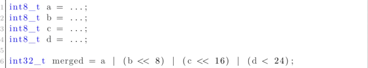
Variable aliasing works by changing the way in which variables are stored, e.g. by splitting them up into several variables or merging them into a single variable. A simple example is the merging of two equally sized integers into one integer with the double size. This can be done by simply storing the first integer in the lower part of the new integer and the second integer in the upper part. Storing the variables in this way generally requires the new variable to be repacked for each operation that operates on either of the original variables. Listing 2.4 shows an example of how variables can be aliased.
Class refactoring
1 int8_t a = . . . ; 2 int8_t b = . . . ; 3 int8_t c = . . . ; 4 int8_t d = . . . ; 5 6 int32_t merged = a | (b << 8) | (c << 16) | (d < 24) ;
Listing 2.4. An example of how four variables can be merged into one.
classes with no real functionality, or by taking all functionality of one class and split it into two new classes while the original class acts as a proxy for the two new classes. Figure 2.7 shows one such example.
1 c l a s s InputCheck { 2 void updateInput( ) ; 3 i n t getResult( ) ; 4 } ; 1 c l a s s A { 2 void updateInput( ) ; 3 } 4 5 c l a s s B { 6 i n t getResult( ) ; 7 } ; 8 9 c l a s s InputCheck : 10 p u b l i c A, B {}
Figure 2.7. Example showing how the code to the left can be transformed
according to the class refactoring obfuscation method. Note that information cannot be shared between class A and B. In case that is needed, diamond inheritance might be required.
Array restructuring
Array restructuring is an obfuscation method that changes the structure of an array, transforming it in a way that makes it difficult for an attacker to understand its structure at run time. A simple example of array restructuring would be reversing it at compile time, and reading it in the opposite order at run time effectively undoing the reversal done during compilation. Listing 2.5 shows an example of array restructuring.
1 i n t scan[ 1 0 ] = { 8 , 2 , 9 , 0 , 6 , 4 , 1 , 3 , 5 , 7 } ;
2 i n t f i b o n a c c i[ 1 0 ] = { 2 , 8 , 1 , 13 , 5 , 21 , 3 , 34 , 0 , 1 } ; 3
4 f o r (i n t i = 0 ; i < 1 0 ; ++i)
5 p r i n t f("%d\n " , f i b o n a c c i[scan[i ] ] ) ;
Listing 2.5. An example of how an array can be restructured for obfuscation
purposes.
Variable promotion
The motivation behind variable promotion is to make it more confusing which context a variable belongs to by increasing the scope of said variable. For example a loop variable is commonly initialized just before the loop, used for array indexing inside the loop and at the end of the loop incremented or decremented. After the loop it is usually not used for anything. Instead of this scheme, an obfuscator can initialize the loop variable implicitly in some other context, use the loop variable in the loop, and then continue to use it outside the loop context, as shown in Listing 2.6.
1 i n t i; 2 f o r (i = 0 ; i < 1 0 ; ++i) 3 check(i) ; 4 5 char b u f f e r[i ] ; 6 s c a n f("%9s " , b u f f e r) ;
Listing 2.6. An example of how a variable can be promoted for obfuscation
purposes.
2.5.3
Control flow obfuscation methods
Control flow obfuscations aim to complicate the control flow graph of a pro-gram. They generally do this by adding more program states and branches. This makes the debugging process of the program more tedious. Some con-trol flow transformations are similar to the transformations that the compiler performs on the code when optimizing it. Some common optimizations may be reverse transformations to control flow obfuscations. Thus clever optimiza-tions may undo control flow obfuscaoptimiza-tions.
Opaque predicates
Opaque predicates are predicates which will evaluate to a, at compile time, known value. Using this fact, we can create conditionals which will complicate the control flow graph. This could be done by e.g. using a mathematical identity as in Listing 2.7 [5]. 1 i n t v = rand( ) ; 2 i f ( (v ∗ v ∗ (v+1) ∗ (v+1) ) % 4 == 0) 3 // always executed 4 e l s e 5 // never executed
Listing 2.7. An example of dynamically created opaque predicates.
An obfuscator could also use relations between variables acquired through e.g. statical analysis to create opaque predicates. The obfuscator could also choose to create such relations itself through the introduction of one or more new variables with a predecided relation.
Opaque predicates are commonly used as part of other obfuscation meth-ods to produce more powerful obfuscations.
Pseudo cycles insertion
Pseudo cycles insertion creates a loop in the code with some kind of opaque predicate as loop condition, which makes the program always break out of the loop immediately, but for a static analyzer it will look like there is another loop in the program. This further complicates the control flow graph of the program.
Control flow flattening
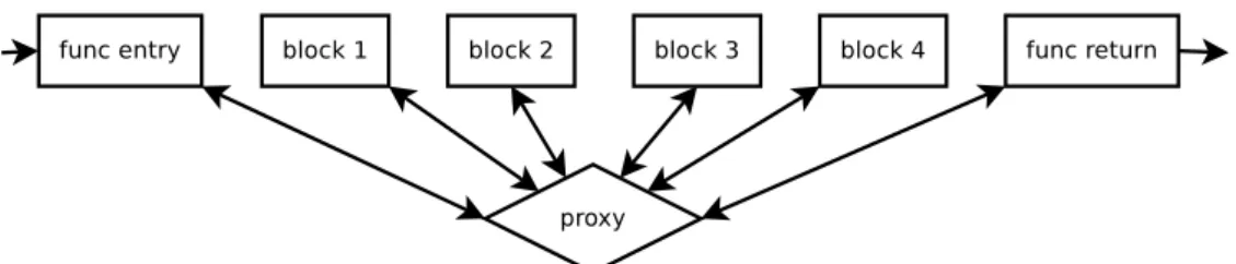
The control flow graph visualizes the program flow and can thus help an at-tacker in understanding the program structure. The control flow can also help to trace at what places in the code a specific function is called. Control flow flattening is a collection of methods for obscuring this structure by reducing the height of the control flow graph. In the extreme case, all jumps between basic blocks in the program are replaced by jumps to a common proxy which relays each jump to its original jump destination. This method effectively reduces the control flow graph to two levels – one level containing all original basic blocks, and one level with the proxy, with edges between the proxy and each basic block entry point and edges between each basic block’s exit point and the proxy entry point, as shown in Figure 2.8.
Figure 2.8. A program where all jumps between basic blocks go through a
common proxy block.
Combined with opaque predicates, this obfuscation method can make it much more difficult for the attacker to determine what path will be executed just through static analysis.
Function pointer obfuscation
All common programming languages have support for function calls. Some programming languages also have support for function pointers. In contrast to normal functions, it may be difficult to determine what function is actually called when a function pointer is used instead.
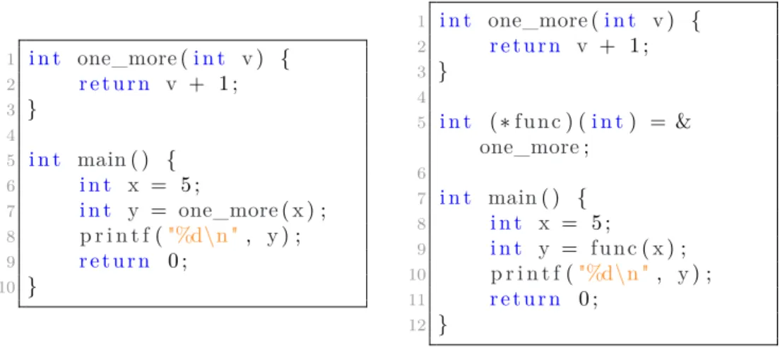
One approach to function pointer obfuscation is to store a pointer to each function in a globally accessible array. Each function call is then replaced by indexing into this array, loading the pointer that corresponds to the function to call and finally calling that function pointer. This scheme can be extended with other obfuscations, such as value encoding and variable aliasing, effec-tively obscuring the function pointer data structure. Combined with opaque predicates, the process of determining statically what function is called can be made even more difficult.
Transforming the code to use function pointers instead of normal function calls have been formally proved to obscure the program. In the general case, determining which function a function pointer call corresponds to has been proven to be NP-hard [23].
Figure 2.9 shows an example of function pointer obfuscation.
Loop transformations
The optimizer in a compiler often performs various loop transformations, for example loop unrolling. Such transformations can also be used by an obfusca-tor to make the code more difficult to understand. Other obfuscations include changing the loop body into a semantically equivalent but more obfuscated
1 i n t one_more(i n t v) { 2 return v + 1 ; 3 } 4 5 i n t main( ) { 6 i n t x = 5 ; 7 i n t y = one_more(x) ; 8 p r i n t f("%d\n " , y) ; 9 return 0 ; 10 } 1 i n t one_more(i n t v) { 2 return v + 1 ; 3 } 4 5 i n t (∗func) (i n t) = & one_more; 6 7 i n t main( ) { 8 i n t x = 5 ; 9 i n t y = func(x) ; 10 p r i n t f("%d\n ", y) ; 11 return 0 ; 12 }
Figure 2.9. An example showing how the code to the left can be obfuscated
with the help of function pointers.
Exceptional branching
Common practice is to use some pattern resembling the if-then-else construct when handling conditional control flow in the application. However, excep-tions can be used for this purpose as well if they are supported. In fact, an if-else construction can be trivially transformed into a semantically equivalent try-catch block.
This type of obfuscation does not really alter the control flow in the most strict meaning, but it alters the construct that determines the control flow. The motivation behind this is mainly that it can be used to obscure a code block so that it looks like normal exception handling code while it in fact is not, thus misleading a reverse engineer.
Figure 2.10 shows an example of an imaginary exceptional branching trans-formation.
Dead code insertion
Dead code is code that is either unreachable during program execution or code that does not do anything useful. The motivation behind adding dead code to the program is that it makes the code less clear. A reverse engineer would have to determine what code is executed before he can make any conclusions about what the code does and how it works. Consequently one of the most important attributes when it comes to dead code insertion is that the code is stealthy, i.e. that it does not stand out to the surrounding code. In the case of
1 i n t check(i n t input) { 2 i f (input > 400 && input
< 800) 3 return 1 ; 4 e l s e { 5 . . . 6 return 0 ; 7 } 8 } 1 i n t check(i n t input) { 2 try { 3 i f (input > 400 && input < 800) 4 throw 1 ; 5 e l s e { 6 . . . 7 return 0 ; 8 } 9 } catch (i n t e) { 10 return 1 ; 11 } 12 }
Figure 2.10. A normal conditional control flow to the left, and code that
uses exceptional branches to the right.
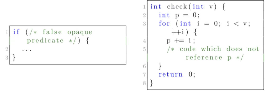
insertion of unreachable code, there is a need for stealthy opaque predicates to protect the code. Figure 2.11 shows unreachable code and useless code.
1 i f (/∗ f a l s e opaque p r e d i c a t e ∗/) { 2 . . . 3 } 1 i n t check(i n t v) { 2 i n t p = 0 ; 3 f o r (i n t i = 0 ; i < v; ++i) { 4 p += i;
5 /∗ code which does not
r e f e r e n c e p ∗/
6 }
7 return 0 ; 8 }
Figure 2.11. Unreachable code to the left, and useless code (the code that
operates onp) to the right.
Dead code can, like opaque predicates, be useful for other obfuscation methods. One such is exceptional branching, where dead code can be placed in unreachable catch blocks for example.
functions sequentially performs the same action as the original function, and transforming blocks of code into functions.
Functions provide a means for an attacker to navigate in a program. If an important function has been discovered by an attacker he can use this function as a starting-point and track down all the callers of this function. Inlining a function makes it more difficult to do such tracking. Splitting a function into multiple functions makes it more difficult for an attacker to grasp the context of the function. Combined with replacing the split functions with pointers as explained in Section 2.5.3, this can be a powerful obfuscation.
Code virtualization
Code virtualization is an obfuscation method in which the code is transformed into virtual machine code. The code is then executed through the use of a virtual machine interpreter that is shipped along with the program. Code virtualization can be applied on the whole program or only on parts of it.
This method is primarily useful for making the program more time consum-ing to reverse engineer. To reverse engineer the obfuscated code an attacker may have to reverse engineer the virtual machine used to run the code. The structure of the virtual machine may be very complex, making this a diffi-cult and tedious task. Running the code in a virtual machine interpreter is typically very slow compared to executing the native code directly, thus this approach may not be suitable for performance critical code.
Encryption
Encryption can be applied on different levels in a program. One approach is to encrypt the program in full, and decrypt it in full upon execution. An attacker can in this case either decrypt the program statically or dump the program just after the decryption in run time. In most cases, only parts of the program need to be protected. In this case the full program need not be encrypted, but only the relevant parts.
Another interesting approach to encrypting a program is to do context dependent encryption. Consider a code block protected by a conditional com-paring a variable to a constant string for equality. If the code block is executed, the variable will definitely have the value of the constant string. Thus we can encrypt the code block with the constant string as key. To make it more dif-ficult for a reverse engineer to do static decryption, the comparison between the variable and the constant string can be replaced by a comparison between the hash of each value. We know that the hash of the string is not enough to decode the block, hence an attacker would have to run the code to be able
to deduce the meaning of the code in question. Listing 2.8 shows an exam-ple of such an approach. Note that this in general requires support from the environment for running self modifying code.
1 i f (hash(input) == hash(" encryption−key ") ) { 2 /∗ Decrypt t h i s block with input as key ∗/ 3 }
Listing 2.8. An example where part of the program has been encrypted based
on a string key. The hashing of the string should be done at compile-time for the best result.
2.6
Obfuscation quality
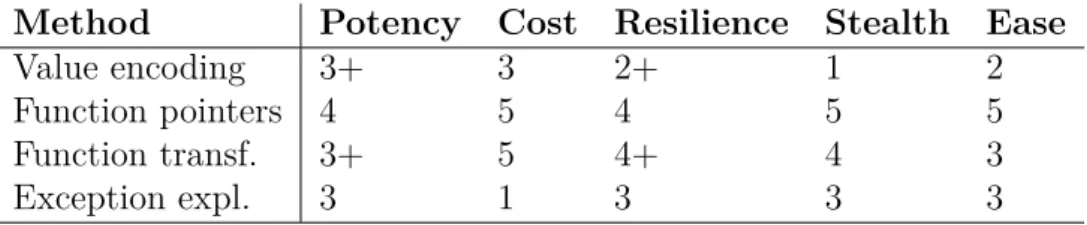
Collberg et al. [4, 5] propose a number of criteria to use when evaluating obfuscation transformations. In particular they define the criteria potency, resilience, execution cost and stealth. Drape [9] added more criteria, of which we were particularly interested in what he defined as ease of integration.
2.6.1
Potency
Potency is defined to measure how obscure a program P is, i.e. how difficult it is for a human reader to understand. It is based on results in software complexity metrics research. Defined are a number of attributes Ei, which
are chosen carefully. The program P is defined to be more potent than the program P0 with regards to the attributee if e(P)/e(P0) >1. Attributes for measuring potency include cyclomatic complexity, program length and nesting level complexity. Collberg proposed that a weighted sumE = Σki·Ei(P) could
be used to retrieve one potency value from multiple metrics.
Cyclomatic complexity
McCabe defined a measure called the cyclomatic complexity number [22]. The purpose of the measure is that when a function is more complex, it will have a higher cyclomatic complexity number.
McCabe showed that the cyclomatic complexity C of a function f can be calculated as
C(f) = ef −nf + 2 (2.2)
where ef and nf denotes the number of edges and nodes respectively in the
where df denotes the number of conditions in the function f.
Applied to a program, the cyclomatic complexity can be calculated by tak-ing the sum of the cyclomatic complexities of all its functions. The argument for this is that a call to a function is just an edge in the control flow graph of a program.
Halstead’s metrics
Halstead defined a number of metrics that can be used for measuring the complexity of a program. For the potency criteria we are interested in one of them, namely Halstead’s difficulty metric. Consider a subset of a program, for example one block in a control flow graph, or a function. Letn1be the number
of distinct operators in the subset. Furthermore let n2 be the number of
distinct operands andN2the total number of operands in the subset. Halstead
proposed a difficulty metric D for the subset defined as in Equation 2.4.
D= n1N2 2n2
(2.4) Halstead claimed that D is positively correlated with the complexity of the subset it is calculated for, and that it can be used to compare different blocks of code with each other.
Nesting level complexity
Harrison et al. [15] argued that neither McCabe’s nor Halstead’s metrics han-dled the complexity added by deep nestling of blocks of code correctly. He suggested that the complexity of a control flow graph block should not only depend on what operands and operators that are contained in that particular block, but also on the complexity of the blocks that the block in question can reach. Harrison does not explicitly specify how his new analysis metric should be carried out.
A more precise definition of a complexity measure based on the same idea is proposed by Gong et al. [12].
Assume that we have a directed control flow graph G of a function, with exactly one entry node and exactly one exit node. Let suc(x) denote the set of immediate successors of x. If and only if|suc(x)|>1, we call x a selection node.
Define postdomination as follows. For two nodes x, y ∈ G, x 6=y, x post-dominates y if and only if every path from y to the exit node passes through
• ∀ z such that z postdominates y, z postdominates x.
We note that trivially all nodes have exactly one direct postdominator when there is only one exit node. For a selection node x, we let Gx contain
all the nodes between x and the node that postdominates it. Let dn be the
number of selection nodes in Gn.
Now, we are ready to define our nesting level complexity measure. The nesting degree of a selection nodex is defined as in Equation 2.5.
n = 1−(1/dn) (2.5)
The nesting degree of the entire graph is calculated as = (1+2 +...+
N)/N, where N is the number of selection nodes in the entire graph. This
will yield a nesting complexity measure between 0 and 1, where higher value means higher complexity.
It is difficult to apply the nesting complexity algorithm on a program (i.e. with function calls as normal edges), because of many reasons (indirect function calls, external function calls, etc). It could be argued however that just as for cyclomatic complexity it is possible to get a good result by simply taking the sum of the nesting complexity of all functions in the program.
2.6.2
Resilience
Resilience is a criteria measuring how difficult it would be to create and execute an automatic deobfuscator for a transformation, reversing the obfuscation per-formed. In contrast to potency this measures the confusion for an automatic deobfuscator, whereas potency measures the confusion for a human deobfus-cator. Evaluation of this criteria is quite subjective and speculative, but may be backed up with formal results.
2.6.3
Execution cost
Execution cost is the penalty in terms of speed and memory that an obfusca-tion imposes. Collberg et al. [4] defined 4 levels for this criteria; free, cheap, costly and dear. An obfuscation is regarded as free if the execution cost is constant, i.e. the penalty is the same regardless of what input the program is run on. It is regarded as cheap if the amount of resources needed to run the obfuscated program is linearly dependent. Define n to be the resources used by the original program, i.e. time and/or memory used. Costly is defined to be any obfuscation that requires O(nx), x > 1, more resources than the original
2.6.4
Stealth
Stealth measures how easily a programmer can determine if and how a partic-ular code has been obfuscated. The motivation behind this criteria is twofold. First, an attacker will probably be more interested in a piece of code that looks obfuscated as it probably has been obfuscated for a reason. Second, if the re-verse engineer can detect what methods were used to obfuscate a program, he can more easily develop inverse transformations to recreate the original code as well as understand the code easier.
2.6.5
Ease of integration
Ease of integration measures how easily an obfuscation can be applied to an existing toolchain. It takes into account how difficult it is to produce an obfuscation tool for the given method, adapt it to the source at hand and include it in an existing toolchain.
Method
In this chapter we discuss the method that we will use for collecting the results. We first state some assumptions about the context of the code obfuscation, then we discuss the implementation of the obfuscation methods in more detail and finally we describe how the evaluation of the code obfuscation methods will be performed.
3.1
Assumptions
The programming language has been assumed to be something similar to C or C++, i.e. statically typed and imperative. It is still possible though that some of the topics discussed are applicable for other programming languages.
3.2
Obfuscation methods
In order to complete the project on time, only a few obfuscation methods could be analyzed in detail. After a brief review regarding the ease of integration, potency and resilience, it was decided that the project should focus on four obfuscation methods, namely:
• Function pointer exploitations. • Function transformations. • Exception exploitaions. • Value encoding.
3.2.1
Function pointer exploitations
Programming languages often have support for direct function calls as well as indirect ones. In particual, C [17], C++ [27], Python [10] and Java [13] support indirect function calls, although Java requires the use of classes to implement it.
The primary reason why indirect calls provide more obfuscation than direct calls is that indirect calls are typically dependent on runtime information. Thus it is potentially much more difficult for a static analyzer to determine which function actually gets called from a particular call site. Wang et al. [31] showed that in the general case, the problem of precisely determining indirect branch addresses is NP-hard. In a more specific case the problem is much simpler though. Consider for example the sample code in Listing 3.1.
1 i n t (∗f u n c t i o n) (void) = other_function; 2 f u n c t i o n( ) ;
Listing 3.1. An indirect call.
Statically determining the exact function that is called in runtime is in this case trivial. An obfuscation scheme that transforms direct calls to indirect calls must thus be more advanced and use more complex strategies.
Wang et al. [31] propose an algorithm for this transformation which uses a global array where function pointers are stored. The array is modified in runtime, e.g. for initialization. To make statical analysis more difficult, initial-ization of a function pointer variable and the call to it are placed in different blocks of code, i.e. different basic blocks. Additionally, they propose that dead code performing arbitrarily complex modifications to the array could be in-troduced to make the problem of statically determining the array’s contents more difficult. The dead code would have to be protected by strong opaque predicates if it should be effective against static analysis.
We follow part of the proposal made by Wang et al. The addresses of each function used in direct calls are placed in an array local to the object file. Additionally this array is used for holding other pointer values, such as pointers to global values. Listing 3.2 shows an example of such an array.
Storing arbitrary pointer values in the array can hinder an attacker to dis-assemble the code into functions. Consider for example a local static function defined inside a file. When compiled into machine code this function will only consist of a sequence of instructions in a binary executable. In order to do the reverse transform, i.e. determining that the sequence of instructions form a function, a disassembler needs to find the start of the function.
1 i n t function_a( ) ; 2 i n t function_b( ) ; 3 i n t g l o b a l _ v a r i a b l e; 4
5 void (∗function_array) (void) [ 5 ] = { 6 p r i n t f , 7 &global_variable , 8 function_a , 9 function_b, 10 function_a , 11 } ;
Listing 3.2. A global array for storing pointer values.
sweep and recursive traversal [25]. Adding bogus instructions before the start of the function can make disassembly with a linear sweep disassembler more difficult. The recursive traversal algorithm recursively disassembles reachable code, and if the function in question is reachable it may be correctly disas-sembled. This process is trivial for direct calls. For indirect calls however, the disassembler will have to perform static analysis to evalute the value of a function pointer in runtime, or fall back to guesses, in order to recurse to a function which only is accessed through indirect calls. If the array storing function pointers also contains pointers to non-functions, then the disassem-bler may make incorrect guesses about what is a function and what is not. For the sake of obfuscation, incorrect disassembly is a good thing as it makes the process of reverse engineering more troublesome for an adversary.
Each direct call to any of the functions stored in the array of function pointers is then replaced with an equivalent indirect call to that particular function through the function pointer stored in the global array.
As proposed by Wang et al., dead code is added for further obfuscation. The dead code is protected by opaque predicates and would change what function will be called if it was to be executed. An example of an obfuscated program is shown in Listing 3.3.
3.2.2
Function transformations
We define function transformations to mean inlining called functions (i.e. callees) into their caller, splitting a function in multiple parts, cloning a func-tion into multiple copies, and combinafunc-tions of these. Defining funcfunc-tion trans-formations in this way means that if a platform has support for functions,
1 i n t function_a( ) ; 2
3 void (∗function_array) (void) [ ] = { 4 . . . , function_a , . . . , 5 } ; 6 7 i n t main( ) { 8 i n t index = some_value; 9 . . . 10 i f (/∗ f a l s e opaque p r e d i c a t e ∗/) { 11 index += /∗ a r b i t r a r y o f f s e t ∗/ 12 } 13 . . . 14 /∗ c a l l function_a ∗/
15 i n t value = (i n t ( ∗ ) ( ) )function_array[index] ( ) ; 16 . . .
17 }
Listing 3.3. An obfuscated call at line 16.
[4] first mentioned this type of obfuscation as Inline and outline methods and
Clone methods. The motivation behind function transformations are described below.
The call graph of part of a program can serve as a tool for an adversary to understand the structure of a program. One target for the obfuscator is thus to hide information about the call graph. In the case of using indirect calls instead of direct ones, as outlined in Section 3.2.1, the result is an obfuscation of the edges in the call graph. Depending on the viewpoint, function pointer exploitation removes edges from the call graph or pollutes the call graph with lots of invalid edges. The nodes in the call graph are however kept intact. With function transformations, new nodes are created (due to cloning), other nodes are decoupled (due to inlining), some edges are collapsed (due to inlining), while other edges are added (due to splitting and inlining). The effect of these transformations is that the original call graph is not preserved. Thus some information is lost in this process. In particular an adversary will find it more difficult to relate multiple functions based on which functions they call.
Many of these transformations are likely to be touched by the optimizer when it is run on the code in a later phase. One of the optimizers most common tasks is for example to detect code that can be inlined. In the case of LLVM, the optimizer will inline code (if the optimization flags allow it) when an analysis finds that the cost of inlining the function is smaller than the benefit it adds [19].
Benefits from inlining include better cache locality and less overhead. The optimization applies the other way around as well, although less common in practice. An optimizer may decide that a piece of code should be split and pushed out into a new function instead. It may also recognize that two functions have equal semantics and replace them with a single function.
All function transformations with the purpose of obfuscating the code must hence have the optimizer in mind so that the transformations are not undone by the optimizer later on in the toolchain. To decrease the possibility of this we perform function transformations in three steps, as described in Listing 3.4.
1 f o r Function f in Program :
2 # i d e n t i f y blocks o f code that can be put i n t o a new f u n c t i o n 3 # and perform t h i s transformation randomly .
4 f = s p l i t F u n c t i o n(f) ; 5
6 # clo ne the r e s u l t i n g f u n c t i o n in a random number o f c l o n e s 7 S = cloneFunction(f) ;
8
9 f o r Function g in S :
10 # i n l i n e a few o f the c a l l s in g , randomly 11 g = i n l i n e C a l l s(g) ;
12
13 # update the c a l l e r s to f to use one o f the transformed 14 # f u n c t i o n s
15 f o r Call c in c a l l s T o(f) : 16 h = random.s e l e c t(S) ; 17 c.setCalledFunction(h) ;
Listing 3.4. Pseudo code for the function transformation algorithm.
The original function is first split up into subfunctions, and the resulting function is cloned. Finally, some randomness is added to the functions through inlining. As there probably will be multiple copies of the function, this reduces the risk that the first split step is reversed by the optimizer. The last step ensures two things. Inlining is likely to collapse two nodes into one in the call graph. It also ensures that the cloned functions are not equal to each other so that static analysis is less likely to detect them as equal. This chance can be further reduced by performing other transformations on the resulting code.
It is essential that the original semantics of the code is preserved when performing function transformations. In particular, local variables shared by multiple instances of the function (i.e. local static variables in C) must continue to be shared. An obfuscator can ensure this by substituting the local variable
3.2.3
Exception exploitations
Drape [9] suggested that exceptions could be used for code obfuscation when it is supported by the programming language at hand. He proposed a couple of transformations from conditional branches to exceptional code. In particular he suggested that an obfuscation pass could perform the transformation from the code in Listing 3.5 to the code in Listing 3.6.
1 A; 2 B;
Listing 3.5. Two sequential statements.
1 try { 2 i f (/∗ f a l s e opaque p r e d i c a t e ∗/) { 3 throw e r r o r; 4 } e l s e { 5 A; 6 } 7 } catch (e r r o r) { 8 /∗ bogus code ∗/ 9 } f i n a l l y { 10 B; 11 }
Listing 3.6. Code which is semantically equivalent to the code in Listing 3.5,
but which uses exceptions for control flow.
This approach, and variations of it have the benefit that the actual control flow is very similar to the original control flow. More specifically, the con-trol flow will not contain exception handling as the exceptional branches are protected by opaque predicates.
Exception handling is very much dependent on the programming language and toolchain used. For example, the C++ ABI (Application Binary Interface) [3] defines how exception handling should work in C++. In particular the exception handling process consists of three phases:
1. Set up an exception handling object, containing information about the exception such as an object thrown and its type.
2. Raise the exception. The implementation unwinds the stack and de-cides where execution should proceed, i.e. which catch block that should handle the exception.
3. Control is passed to a relevant catch block, which may or may not trigger a new exception.
As the destination catch block is runtime dependent, there is no way to tell which catch block will resume execution without some static analysis on the type of the thrown object and the available catch blocks. Thus if the target ABI is the C++ ABI for an obfuscated build, an obfuscator can exploit the inherently complex exception handling mechanism for obfuscation purposes. One example of this is to change the control flow such that the normal control flow path will trigger exceptions and rely on correct exception handling, as shown in Listing 3.7. 1 try { 2 i f (/∗ true opaque p r e d i c a t e ∗/) { 3 throw e r r o r; 4 } e l s e { 5 /∗ bogus code ∗/ 6 } 7 } catch (e r r o r) { 8 A; 9 } f i n a l l y { 10 B; 11 }
Listing 3.7. Code which is semantically equivalent to the code in Listing 3.6,
but in which the normal control flow path will trigger exceptions.
There is a negative side effect of letting the exceptional path be part of the actual control flow path though. In particular exceptions usually have a large impact on the speed of a program. The exact impact varies between ABI’s and implementations.
Our implementation combines transformations similar to those shown in Listing 3.6 and 3.7.
3.2.4
Value encoding
Collberg et al. [4] mentioned value encoding as a method to protect a pro-gram’s values and constants from an adversary. Consider for example the code in Listing 3.8.
In the context of the code in Listing 3.8 the value 4412 is special and may be a target for an adversary. Value encoding is a transformation that conceals the constant while keeping the semantics intact. Collberg did not
1 i n t check_input(i n t input) 2 {
3 return input == 4412;
4 }
Listing 3.8. Sample code showing a function that validates the input.
depending on context, usage, and other factors. Consider for example the code given in Listing 3.9.
1 i n t check_input(i n t input) 2 {
3 i n t constant = 4412 ^ 1234; 4 return input == constant ^ 1234; 5 }
Listing 3.9. An example of value encoding. This code is semantically
equivalent to the code in Listing 3.8
The code in Listing 3.8 and 3.9 are semantically equivalent. In this par-ticular example the value encoding function is ⊕with a constant value 1234. ⊕ is special in that it is the inverse of itself, but any injective function which works on the domain in question can be used. For the purpose of this report we identified two operators that can be used for encoding integer values.
• ⊕ – The second operand in the exclusive or operation can be randomly selected from the range of the first operand’s type.
• + – The second operand can be randomly selected from the range of the first operand’s type. To do the inverse operation, arithmetic minus is applied. Note that this operator assumes that the definition of integer overflow has certain properties. This may or may not work depending on target platform and toolchain.
Naturally, integer types (including pointers) can be encoded with the method defined above. We do not consider floating point types for obfus-cation in this report, as they have much more complex semantics. Below we specify how we defined the method to encode arrays and compound types. We also discuss how the obfuscator handles pointers to encoded variables.