Optimization of Random Forest Based Methods Applying the Genetic Algorithms

(1)

Optimization of Random Forest Based

Methods Applying the Genetic

Algorithms

Zahra Aback

A Thesis

In

The Department

of

Mathematics and Statistics

Presented in Partial Fulfilment of the Requirements

for the degree of Master of Science (Mathematics) at

Concordia University

Montreal, Quebec, Canada

July, 2018

c

(2)

CONCORDIA UNIVERSITY

School of Graduate Studies

This is to certify that the thesis prepared

By: Zahra Aback

Entitled: Optimization of Random Forest Based Models Applying Genetic Algorithms

and submitted in partial fulfillment of the requirements for the degree of

Master of Science (Mathematics)

complies with the regulations of the University and meets the accepted standards with respect to originality and quality.

Signed by the final examining committee:

Examiner Dr. Yogendra P. Chaubey Examiner Dr. Frédéric Godin Thesis Supervisor Dr. Arusharka Sen Approved by

Chair of Department or Graduate Program Director

Dean of Faculty

(3)

ABSTRACT

Optimization of Random Forest Based Models Applying Genetic Algorithms Zahra Aback

In this century access to large and complex datasets is much easier. These datasets are large in dimension and volume, and researchers are interested in methods that are able to handle this type of data and at the same time produce accurate results. Machine learning methods are particularly efficient for this type of data, where the emphasis is on data analysis, and not on fitting a statistical model. A very popular method from this group is Random Forests which have been applied in different areas of study on two types of problems: classification and regression. The former is more popular, while the latter can be applied for data analysis. Moreover, many efficient techniques for missing value imputation were added to Random Forest over time. One of these methods which can handle all types of variables is MissForest. There are several studies that applied different approaches to improve the performance of classification type of Random Forests, but there are not many studies available for regression type. In the present study, it is evaluated if the performance of regression type of Random Forests and MissForests could be improved by applying Genetic Algorithms as an optimization method. The experiments were conducted on five datasets to minimize the mean square error (MSE) of the Random Forest and imputation errors of the MissForest. The results showed the superiority of the proposed method in comparison to the classical Random Forest methods.

(4)

Acknowledgements

Firstly, I would like to express my sincere gratitude to my adviser Dr. Arusharka Sen for his guidance and all his support for my Master’s studies.

Besides my adviser, I would like to thank my examiners: Dr. Yogendra P. Chaubey and Dr. Frédéric Godin for their precious comments which helped me to improve my research. I would also like to express my gratitude to the faculty members and graduate students who helped me through my studies at Concordia University.

Last but not the least, I would like to thank my family especially my mom and friends for supporting me throughout the writing of this thesis and my life in general.

(5)

List of Figures

2.1 Sample Regression Decision Tree . . . 11

3.1 The process of GA . . . 29

3.2 Blend crossover (BLX−β) method . . . 35

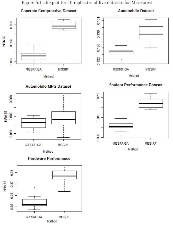
5.1 Boxplot for 10 replicates of five datasets for MissForest . . . 49

(8)

List of Tables

2.1 Regression Random Forest Algorithm . . . 14

4.1 Compute fitness function for MissForest . . . 39

4.2 Genetic Algorithm Process . . . 40

4.3 GA parameters for optimizing MissForest . . . 41

4.4 GA parameters for optimizing RF . . . 42

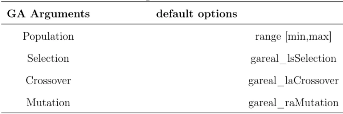
4.5 GA arguments for RF and MissRF . . . 43

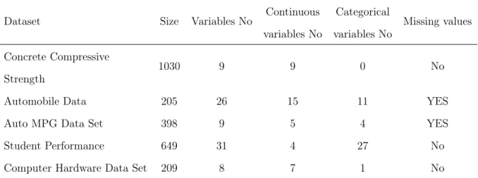
5.1 Description of the datasets used in the experiments . . . 45

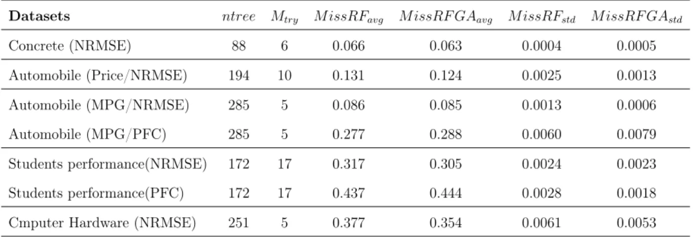
5.2 Comparing imputation error of optimized and classic MissForest . . . 47

5.3 Experimental Results of imputation error for MissForest . . . 47

5.4 Two sets of solutions for optimized MissForest . . . 48

5.5 Comparing Performance of Optimized and classic RF . . . 50

5.6 Experimental Results for Random Forest . . . 51

5.7 Different GA operators for selection, crossover, mutation . . . 53

5.8 Comparing different GA control parameters of RRFGA on Automobile dataset . . . 55

(9)

Chapter 1

Introduction

In the era where we have access to the large volume of data, researchers are looking for methods or algorithms that are flexible enough to handle this type of data for analysis and at the same time produce efficient statistics (Biau & Scornet, 2016). These methods are recently developed in statistics and computer science in parallel which are linked to an area of study called machine learning. This field of study enables computers to learn without being programmed explicitly (Samuel, 1959). Many methods such as classification and regression trees, bagging, and an improved version of them, Random Forests (RF), fall in this category (James et al., 2013).

RF which was introduced by Breiman et al. (2001) has shown a great success in recent decades to handle large datasets. RF has become very popular in recent years since it is applicable in many prediction problems, and much simpler than some other machine learning methods to run due to small number of parameters for tuning. It is also recognized as a method that can be executed in parallel (Biau & Scornet, 2016). RF is a combination of lots of trees that are grown from different pieces of datasets and provides an estimate by averaging over trees (Biau & Scornet, 2016).

Since most of the time it is very common to have datasets that include missing values, we have to decide how to deal with them. This is a very important issue when RF is applied for data analysis since it cannot perform and produce results when missing values are present. In this case, missing values are either discarded if applicable or a decision is made to impute them. There are many imputation methods, but a very few of them

(10)

can handle missing values for both categorical and continuous variables. In this regard, we used MissForest which was introduced by Stekhoven and Bühlmann (2011). Using this method, missing values were imputed and imputation errors were reported for both continuous and categorical variables.

There are two types of Random Forests: classification and regression for categorical and continuous responses, respectively. The regression type of RF produces a predicted value which is the average of the results of all the trees, and its performance is measured by mean square error (MSE) of that estimation.

There are lots of studies focusing on improving the performance of RF or studying the options for its parameter settings that help produce results in a reasonable time frame that are accurate enough. Oshiro et al. (2012) and Latinne et al. (2001) studied the number of trees required in a Random Forest and the first study suggested 64 trees, and the second one suggested limited numbers for different datasets. Their study showed that the number of trees larger than what they suggest will not improve RF performance. Bader-El-Den and Gaber (2012) and Elyan and Gaber (2017) also studied the impact of using Genetic Algorithms (GA) on the improvement of the performance of RF. These studies focused on classification type of RF, the response of which is categorical, and they suggest different approaches.

In this study the focus is on improving the performance of regression RF by applying Genetic Algorithms. In fact, GA is applied to minimize the mean square error of RF by searching over number of trees and number of features at each split. Moreover, it has been studied if GA has an impact on the performance of MissForest to minimize its imputation errors.

1

Random Forest

The RF was devised by Breiman et al. (2001) since he wanted to improve the perfor-mance of Bagging which is the combination of large number of trees that are produced from bootstrap samples of the original dataset. The improvement in comparison to Bag-ging occurred to produce a RF by adding another type of randomness in the model beside

(11)

bootstrap sampling. The other randomness is CART-split, which is choosing the best variable for splitting. The variable is selected from a number of variables in the subset Mtry of total number of variables pto divide the sample space to sub-samples.

The RF is an ensemble method too, which is a method that produces the prediction model (RF) from the strength of the collection of simpler ones (Decision Trees). In fact, ensemble learning includes two procedures. It develops a large number of individual mod-els and then it produces the final prediction by combining them (Friedman, Hastie, & Tibshirani, 2001).

The RF is very efficient when the number of variables is larger than the number of observations, and it is called "off the shelf" method which means it can give a very preliminary result about the dataset in a very short time (Cutler, Cutler, & Stevens, 2012). It does not need any formal assumption about the distribution of the data, and produces proximity matrices which can be used for missing values imputation and for the detection of outliers. It is robust to the outliers. The performance of a RF is measured internally during the implementation of its function, and it ranks the variables by their importance (Cutler et al., 2012). There are many softwares that can implement the RF analysis in their environment such as R. There is a package in R called Random Forest which can be installed to carry out its function and produce the results. In addition to these cases, there are some other softwares that have been developed just for machine learning methods such as Salford Systems Data Mining and Predictive Analytics Software (SPM) and Waikato Environment for Knowledge Analysis (WEKA).

2

Genetic Algorithms

There are many situations in our lives where we are looking for optimization of our performance. For instance, we would like to have maximum sleep but at the same time arrive at work on time. We could think of which route to take or how to be well prepared the night before for the next morning. In fact, we look for a way to minimize our cost and maximize our output or result. Optimization is a process in which the inputs of a mathematical function or experiment or characteristics of a device are adjusted to find

(12)

the maximum or minimum results, see Haupt and Haupt (2004).

Haupt and Haupt (2004) addressed some issues in optimization problems such as finding solutions in the case where the derivative of the objective function (the function that needs to be optimized) does not exist or difficult to derive. Also, the type of solution to the optimization problem is crucial too. It is important to know if the optimum value obtained by this process is local or global.

There are several approaches for optimization with different advantages and disadvan-tages. Haupt and Haupt (2004) discussed many algorithms that help to find the maximum or minimum of some functions that were not either linear nor having a derivatives (it is hard to find their derivative). However, they had one thing in common: they could not produce the global minimum or maximum. Therefore, later some other algorithms were introduced to overcome this problem, among which GA proposed. The GA does not need derivative of the functions and could produce the global optimized solutions to the prob-lems.

John Holland was the first person who tried to develop a theoretical basis for GA. He developed it between 1960s and 1970s and the work was summarized in his book "Adaptation in Natural and Artificial Systems (1975)". However, this method was made very popular through one of his students, David Goldberg (1989), whose dissertation solved a problem which was the control of gas pipline transmission (Haupt & Haupt, 2004).

In their book (Haupt & Haupt, 2004) defined GA as an optimization procedure that imitates the reproduction process in organisms and uses its natural selection method to find the optimum solution. In this process a large population is evolved through a specific selection method to a point that optimizes the fitness function. GA mostly has been used for optimizing hard and complex problems.

3

Missing values

Most of the time datasets are not complete and they contain missing values. There are three most important type of missing values: Completely Missing at Random, Missing at

(13)

Random, and Not missing at Random which are explained as follows:

• Missing Completely At Random (MCAR): If the probability for a variable to have some missing values is independent of other variables, that is called MCAR. In fact, all the observations for a random variable have the same chance of being missing. In this case, missing values can be removed from the dataset without imposing a bias to the estimation, but this type of missing is not very common (Tang, 2017).

• Missing At Random (MAR): If the probability of being missing for a random variable depends on the information of the other variables, it is called Missing At Random. For instance, the information for occupation is missing for some races or ethnic groups (Young, 2017).

• Missing Not At Random (MNAR): If the probability of being missing for a variable is because of that variable itself, it is called MNAR. In this case the respondent is not willing to answer the question because they are embarrassed or they do not want to share their information for that question. Most of the time it is difficult to identify this type of missing since it depends on some unobserved values (Young, 2017).

There are different strategies to deal with missing values. The first one is to remove all the missing values and work with the complete dataset. In this case some information will be lost and we will have larger standard errors. Also, it causes a problem when there is a large number of variables with lots of missing values. In this case discarding these observations will lead to dealing with many variables and few observations. The other approach is to keep missing values and impute them by some current methods, so those parts of the data will not be lost but adjusted (Young, 2017).

There are different methods for imputation, and some of them are RF based methods. The two methods which can be implemented through the RF package in R are rough imputation and RF imputation. The first model replaces missing values by the median or the mode and produces the imputed values. The second model uses proximity measures in a RF to impute the missing values, but this method cannot be applied when missing

(14)

values are present for the response variable.

The third RF based method is MissForest, some characteristics of which was high-lighted by Stekhoven and Bühlmann (2011). Firstly, this method can handle both cat-egorical and continuous variables simultaneously. Secondly, the imputation error can be computed internally during the imputation process. Finally, it performs really well when non-linear relations or complex interactions are present. A comparison among these three methods shows that the later can produce better results. Therefore, in this study, miss-ing values are imputed by MissForest, and it was also studied if GA can optimize its performance by minimizing imputation error (Stekhoven & Bühlmann, 2011).

4

Limitation

There are two types of RFs, a classification RF and the regression one, and most of the time the focus in studies was always on the classification type. Some of these studies focused on two parameters in RF that are considered as the most important factors which have an effect on the its performance: the number of trees and the number of features considered at each split (Elyan & Gaber, 2017). There are some studies that looked for reducing the number of trees to produce accurate results but at the same time reduce the processing time (Oshiro et al., 2012). Some other studies tried to find the best values for the number of features considered at each split that could produce better results than default values of a given RF implementation (Bernard et al., 2008). Also, two studies focused on finding the best values for both parameters mentioned above to minimize the model error by applying an optimization method, GA (Bader-El-Den & Gaber, 2012), Elyan and Gaber (2017).

In spite of the fact that regression RF follows the same routine as the classification type, according to my knowledge, there are not many studies available on evaluating the performance of a regression RF. Therefore, the objective of the current study is to evaluate if the mean square error of the regression RF could be minimized by searching over the optimal numbers of trees and number of features at each split. GA was applied as an optimization method to produce the minimum error and report its corresponding

(15)

solutions. This method was selected since it could optimize complex functions, it could produce the global optimal solution, and it could be run in parallel. Moreover, since MissForest is also an RF based model for the imputation, the other objective is to study if its performance could be improved (minimizing the imputation error) by finding the optimal solutions for the number of trees and the number of features at each split.

(16)

Chapter 2

Random Forest

The early definition of a Random Forest that is given by Breiman (2001) was for a classification RF and was expressed as follows:

A Random Forest is a classifier that is created by a group of trees {h(x,Θk) k =

1,2,· · · }where the{Θk}are identically independent random vectors, and each tree votes for the most popular class for an input x. The random vector Θk is not defined in this work, but implicitly it represent two types of randomness in an RF including the Bagging and splitting a node which will be explained later.

A regression Random Forest is similar to a classification one, except that for an input x, each tree produces an average as the estimation. The process of producing the esti-mation for a regression RF will be explained in details later. The most important factors in building a RF are CART-split of a Decision Tree and Bagging which creates predic-tors from bootstrap samples of the original dataset and produces the final estimation by averaging them (Biau & Scornet, 2016).

1

Decision Tree

The most popular Decision Tree is a Classification and Regression Tree (CART) that was introduced in 1984 by Leo Breiman, Jerome Friedman, Richard Olshen and Charles Stone. In this method the response could be continuous or discrete that leads to a regres-sion or classification tree respectively.

(17)

1.1

CART-Split

In tree-based methods, the sample space is divided into a set of sub-spaces which are called regions or nodes and each of them creates an estimate (Friedman et al., 2001). The process of dividing the whole sample space into regions is called CART-split which is a procedure that a variable and best value of that is selected from a whole set of variables to minimize the mean square error of a region (Biau & Scornet, 2016).

CART-split of a Decision Tree is a binary partitioning of a sample dataset of size n, _Dn, and in each step it splits each region into two regions on the left and right by minimizing the mean square error of those regions for a regression tree. For instance for a (subset) region A suppose the number of observation is Nn(A) and the pair of (j, z) as a cut point in which the splitting occurs. The component j of the pair refers to the co-ordinate variable Xj so that, this variable is selected from a whole set of independent variables (X1, X2,· · · , Xp) where p is the number of predictors. The second component z is a value from the domain of variable Xj where the splitting occures. This region will be divided into two more regions based on the best pair from whole predictors and their best splitting values. If _CA denotes a set of all pairs of cuts, the regression CART-split criterion that leads to growing a tree from top to down for each pair (j, z)_CA by consideringXi = (Xi1, Xi2,· · · , X

p

i)where i= 1,2,· · ·, n is in the from in Equation (1.1): (Biau & Scornet, 2016):

Lreg,n(j, z) = 1 Nn(A) n X i=1 (Yi−Y¯)2IXiA− 1 Nn(A) n X i=1 (Yi−Y¯ALIX_ij<z−Y¯ARIX_ij≥z) 2_I XiA (1.1)

The variable Yi is the response variable correspond to all the Xi in each region and

¯

Y is the average of all the Yi in that region, which is obtained by minimizing the mean square error of that region. The Equation (1.1) above has to be maximized to find the best variable and best value from its domain as the cut.

Region A is divided into two regions on the right AR = {XA :Xj ≥ z} and on the left AL={XA:Xj < z}. For region A, Y¯ is obtained from all the Yi corresponds toXi in region A and Y¯AL and Y¯AR respectively calculated from Yi corresponding to the Xi in

(18)

regions AL and AR. This process will be repeated for the next regions and each time a best cut at the pair of (j?, z?) will be selected by maximizing the Lreg,n(j, z) over set of all the pairs so that the best cut is defined as below:

(j?, z?)∈arg max

j∈{1,2,···,p}

(j,z)∈CA

Lreg,n(j, z) (1.2) As it can be observed, at each node the criterion (1.1) is evaluated and the best cut at each split is determined. The best cut in Equation (1.2) is not a unique pair and each time for each split it changes and produces different values. Equation (1.1) was first used by (Breiman et al, 1984) which measured the variance before and after splitting (Biau & Scornet, 2016).

1.2

Estimation

The general idea is to produce a non-parametric regression estimation. The goal is to predict the random response Y ∈ _R where E(Y2 _<_∞₎ _{by estimating this regression}

function m(x) = E[Y|X = x] for an input Random vector X ∈ χ where χ is an input space. Having this in mind, for a sample dataset_Dn = ((X1, Y1),(X2, Y2), . . .(Xn, Yn))the estimate mn : χ −→ R is constructed for the function m. The estimate for a regression random tree at a value x is defined as follows:

mn(x,Dn) = X i{1,2,···,n} I_XiAn(x,Dn)Yi Nn(x,Dn) (1.3)

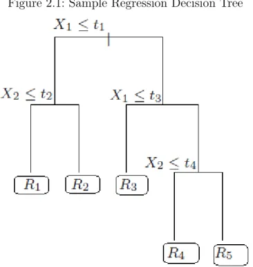
whereAn(x,_Dn)is the region that containsxandNn(x,Dn)is the number of observa-tions that belong to the region An(x,Dn). This estimation is the average of the responses in a region, An(x,Dn), where the new input x has fallen (Biau & Scornet, 2016). The process of CART-split (Friedman et al., 2001) for a sample dataset with two random variables X1 and X2 is depicted in Figure 2.1 (Friedman et al., 2001).

(19)

Figure 2.1: Sample Regression Decision Tree

As displayed in Figure 2.1, at first, the sample space was divided into two regions. Next, as depicted in Figure 2.1, the next region on the left also splitted to two more regions and stopped from splitting in regionsR1 and R2 which are called terminal nodes.

Then, the corresponding region on the right was divided into two more regions and it continued splitting until the number of observations in each node (node size) is less than 5 or the stopping criterion is met (Friedman et al., 2001).

Decision Trees produce estimations with high variance, such that a small change in the dataset will result in a different splitting, which leads to an unstable interpretation of the tree (Friedman et al., 2001), so Bagging was introduced to alleviate this problem.

2

Bagging

Bagging which is the abbreviation of a bootstrap aggregation is known to work well for low-bias and high-variance models like Decision Trees (Friedman et al., 2001). It was introduced by Breiman (1996) and is a procedure in which many trees are built by drawing several bootstrap samples from the dataset and by applying CART-split procedure from Decision Trees on each bootstrap sample. In this process, each tree produces an estimate,

(20)

and the final prediction is obtained by averaging over these estimates. Bootstrap sampling which introduced by Efron (1979) is a process of producing several samples of the original dataset with replacement.

In a Bagging procedure, trees are grown from bootstrap samples. In this process, a bootstrap sample of _Dj

n, j ∈ {1,2,· · · , M}from a sample datasetDn is drawn and a tree is grown for this bootstrap sample. Then, if prediction of a bagging tree is m?

n(x,Djn) as defined in Equation (1.3), then, the final prediction for Bagging from all trees,ntree=M, is: mM,n(x,Dn) = 1 M M X j=1 m?_n(x,_Dj_n)

The most important point in Bagging is to obtain a smaller variance by averaging over many noisy but approximately unbiased trees. Trees are a perfect option for Bagging because they can capture the complex interactions in the data with relatively low bias if they grow deep enough (Friedman et al., 2001). Trees that are grown in Bagging are identically distributed, and the expectation of the average of trees is the same as a Decision Tree, so the only hope is to reduce variance. Since trees are identically distributed but not necessarily independent, the variance of the average of their estimate for ntree =M trees is (Friedman et al., 2001):

V ar( 1 M M X j=1 m?_n(x,_Dj_n) = 1 M2V ar( M X j=1 m?_n(x,_Dj_n)) = 1 M2{M σ 2₊_M₍_M ₋₁₎_ρσ2_}₌_ρσ2₊ 1−ρ M σ 2 (2.1)

In Equation (2.1),ρis the correlation between the predictions for an inputxprovided by two trees from the bagging procedure. Also, in this equation,σ2represents the variance of the response prediction for an inputxfor each tree in the Bagging model. The variance of Bagging as it is depicted is a composite of two terms. Friedman et al. (2001) explains that when number of trees increases, the second term disappears, and the variance of the predictor just depends on the first term. However, even if second term disappears by increasing the number of trees, it will not be helpful when trees are highly correlated. In

(21)

this case RF was introduced to reduce the correlation between trees without increasing the variance from predictions of the various trees too much.

3

Regression RF and its characteristics

A regression RF is built by applying Bagging and CART-split procedures from last two sections. In the CART-split process the variable for splitting is selected from whole set of variables{X1_{, X}2_,_{· · ·} _{, X}p_}_{. However, in a RF the splitting variable is selected from}

{X1_{, X}2_,_{· · ·} _{, X}Mtry_} _where _M

try is the number of selected variables at each split.

3.1

CART-Split

The CART-split process for a RF is different from Bagging such that for all the pair of (j, z)_CA the dimension j? is selected from Mtry. Therefore, the best cut for a RF is depicted in Equation (3.1) (Biau & Scornet, 2016):

(j?, z?)∈arg max

j∈Mtry

(j,z)∈_CA

Lreg,n(j, z) (3.1) When the splitting process starts, each time the criterion (2.1) is evaluated at each node, and the best cut which changes at each split is determined (Biau & Scornet, 2016).

3.2

Estimation

The estimation for a regression RF is very similar to Bagging, but the only difference is that in a RF another type of randomness is injected to the model by choosing a random variable from a subset of variables {X1, X2,· · · , XMtry_}_{to start splitting at each node. If} the _Dj_n, j∈ {1,2,· · · , M} is the bootstrap sample for a sample dataset_Dn, the estimate for a regression random tree, j, in a RF is defined at a value x of random variable X as follows (Biau & Scornet, 2016):

mn(x; Θj,Djn) = X i{1,2,···,n} I XiAn(x;Θ_{j ,}Djn)Yi Nn(x;Θj,Djn) (3.2)

(22)

where An(x; Θj,Djn) is the region that contains x and Nn(x; Θj,Dגn) is the number of observations that belong to that region. Also, Θ1,Θ2, . . . ,ΘM are the parameters that inject the randomness by Bagging and by selecting a variable Xj, a random variable from a subset of variables, that maximizes Equation (1.1) (Cutler et al., 2012). The estimate for the RF is the average of ntree = M trees estimates and it is depicted in Equation (3.3): mM,n(x; Θ1, . . . ,ΘM,Dn) = 1 M M X j=1 mn(x; Θj,Djn) (3.3) The average is obtained over the whole number of trees. The algorithm of producing a Random Forest (Friedman et al., 2001) is displayed below (see Table 2.1):

Table 2.1: Regression Random Forest Algorithm 1) For j = 1 toM (number of trees)

Draw bootstrap sample _Dj

n of size n from sample datasetDn

Grow a random tree from the bootstrap sample by repeating the next steps recursively for each terminal node until the size of each node is nmin = 5

i) Select Mtry variables randomly from the p variables

ii) select the best variable with the best split value from Mtry that maximizes the Equation (1.1) iii) split the node into two sub-nodes according to the criterion in step ii

2) Output the estimation for all the trees

Prediction for an RF:

mM,n(x; Θ1, . . . ,ΘM,Dn) = _M1 PM_j₌₁mn(x; Θj,Djn)

SinceM could be any number, it could approach to infinity, so the Equation (3.3) for the RF will approach to the parameter in Equation (3.4):

lim

M→∞mM,n(x; Θ1,Θ2, . . . ,ΘN,Dn) = m∞(x;Dn) =EΘ[mn(x; Θ,Dn)] (3.4)

(23)

law of large number justifies the operator limN→∞ (Biau & Scornet, 2016).

A RF and a Decision Tree are varying in three different ways. Firstly, in an RF the best variable Xj and best value of its domain is selected from number of variables in the subset Mtry while in a Decision Tree it is selected from whole set of variables. Second, in an RF, trees are fully grown without pruning1_{, but a Decision Tree is pruned to have a}

better estimate. Finally in a RF, trees are built from a bootstrap sample of the dataset, but a Decision Tree is built from a sample dataste (Biau & Scornet, 2016). Friedman et al. (2001) explained that having the ability to change Mtry could have an effect on reducing the correlation between trees and reducing the variance. They pointed out Breiman et al. (2001)’s suggestion for Mtry which was √p for classification and p/3 for regression. However these numbers could change with respect to problem at hand, so sometimes it can be observed that some other numbers for Mtry produce better results.

In the R package the default value for number of trees is 500, and the default number for theMtry isp/3for a regression RF. Also, the maximal node size which is the stopping point for splitting for a regression RF is 5; at this point the node will not be split further and the node is regarded as a terminal node. Moreover, the repeating sample size for bootstrap sampling is the same as the size of the data set. Sometimes parameters like node size, size of a tree, and the size of the bootstrap considered as tuning parameters that have an effect on the performance of the RF (Biau & Scornet, 2016).

4

Measuring the performance of a regression model

In Statistical learning the goal is to estimate a responseY by discovering its relation-ship with some predictors {X1_{, X}2_,_{· · ·} _{, X}p_}_{. The relationship between these components} is displayed in Equation (4.1) James et al. (2013) :

Y =f(X) +ε (4.1)

As it was defined by James et al. (2013)f would be considered as an unknown function 1_{Pruning is a process in which some of the nodes are removed from the tree and the model error is} evaluated so that the new pruned tree with the least error is selected.

(24)

but fixed and ε was considered a random error with E(ε) = 0 and V ar(ε) =σ2. Also, f represents a mechanism in which {X1, X2,· · · , Xp} disclose some information about Y. The prediction ofY isYˆ = ˆf(X) wherefˆis an estimation of f. There are two quantities that have effect on the accuracy of Yˆ, which are called irreducible and reducible errors. Since fˆ is not always an ideal estimate of f, it introduces some error which is called reducible error. The error is reducible since by fitting a proper model, the error can be reduced. However, even the model is appropriate enough such thatYˆ =f(X), some error is present which is called irreducible error. The reason for this error to be present is that Y is also a function ofε and even if the model performs well, the error that is introduced byεcannot be reduced. This error could be present due to some reasons like not including some variables in the model or it is because of some variation in ε(James et al., 2013). If

ˆ

f is an estimate for f, the mean square error of that can be calculated as it is defined in Equation (4.2). It is also considered as a measure of performance:

E( ˆY −Y)2 =E(f(X) +ε−fˆ(X))2 =E((f(X)−fˆ(X))2) +V ar(ε). (4.2) As James et al. (2013) explained, the first part is the reducible error which can be minimized by applying a proper model and the last part is irreducible error which is out of control. Actually, the most common criterion to measure the regression performance is Mean Square Error (MSE) and when the model is fitted to the sample data it is computed as depicted in Equation (4.3): ˆ M SE = 1 n n X i=1 (yi−yˆi)2 = 1 n n X i=1 (yi−fˆ(xi))2. (4.3) James et al. (2013) named the MSE in Equation (4.3) as the MSE for training data or training MSE. The training data is the one that was used to develop or train the model and it shows how much fˆ(xi) is close to f(xi). If the difference between these two functions is very small it implies that the model performed well on the training data and the prediction is close to the observed value. However, the main interest is not really on the performance of a model on training data. The goal is to see if this model performs

(25)

well on a new data which is called a test data and is independent from the training data. James et al. (2013) pointed out to the fact that when a model fits well on a dataset, it is a positive point, but we are more interested to see if it has the same or close performance on a new similar dataset. For instance, if we have a number of patients with their clinical measurements and we want to predict the risk of diabetes, a model can be applied for this data and fits the data very well, but we want to use this model for future patients and predict the risk of diabetes based on their inputs.

James et al. (2013) described how the MSE for a new observation from a new dataset is computed. They explained when a model is developed by training data, the goal is to find iffˆ(x0)can produce an accurate estimate for f(x0)which is the prediction for a new

observation x0. To measure the performance of a model on a new observation, the MSE

of that is computed by Equation (4.4) which is called a generalization error:

E(y0−f(x0))2 =var( ˆf(x0)) + [bias( ˆf(x0)]2+var(ε). (4.4)

In Equation (4.4) the goal is to reduce the variance and bias as much as possible to have a better performance for the model. However, somtimes it has to be decided for a trade-off between these two factors. Generally, a test dataset is not available to measure the performance of a model, so when we have enough observations it is recommended to divide the dataset into two parts one for training and one for testing. If the performance of the model is assessed on the test set, most of the time its MSE is larger than the training MSE because some of the patterns that have been caught in the training set could not exist in a test set as they are purely due to noise, and this is called overfitting. Although it has to be noted that whether overfitting is present or not, the test MSE is larger than the training MSE because the model directly or indirectly tries to minimize the training MSE. In general, when the test MSE is much larger than the training MSE it is regarded as overfitting (James et al., 2013).

Friedman et al. (2001) also introduced another way of performing data partitioning. They suggested that we have two goals in modeling which are either model selection or model assessment. In model selection the performance of different models could be

(26)

compared to select the best model. In model assessment, the final model would be selected by estimating the generalization error on new data. If we want to address both needs, the best way is to divide the dataset into three parts which are training, validation, and test sets. The training set is used for developing the model, the validation set is used for model selection by estimating the prediction error, and the test set is used to evaluate the generalization error of the final model. There is no specific rule stating how to split the data into the three subsets, and it depends on the size of the dataset and some other factors, but one of the suggestions provided by Friedman et al. (2001) is to divide it to

50%, 25%, 25% of the data for training, validation, and test sets.

5

Out of Bag Error

As discussed in previous section, one of the ways to evaluate the performance of a model is to measure the MSE on a test set which most of the time is not available. In Random Forest this problem has been addressed by measuring the out of bag error which is the MSE of the test data that is available internally during the process of growing trees using bootstrap sampling.

When Bootstrap sampling procedure is applied to grow a tree, about one third of data is not included in the sample and they are regarded as out of bag observations. In fact, for each Bootstrap sample a tree is grown using two third of the sample and out of bag observations are the one third left out observations. These observations are used as a test set to measure the performance of the model (Cutler et al., 2012). The reason that one third of the data is dropped out of sampling as Louppe (2014) described is because after n draw with replacement the probability of not being selected can be calculated as expressed in Equation (5.1):

(1− 1

n) n_≈ 1

e ≈0.368. (5.1)

As Cutler et al. (2012) described these observations are used to assess the performance of the model by estimating the out of bag error. In fact, each of these observations are dropped from the tree, after ending up in a node, the prediction for them will be

(27)

cal-culated, so the mean square error can be computed. If _Dj_n is the bootstrap sample and

\

mn(xi; Θj,_Djn) is the prediction at xi for tree j and the set of out of bag observations is defined as : υi = {j : (xi, yi) 6∈ _Dj

n} and the number of the members of the set is ιi then out of bag estimation is defined as below:

ˆ foob(xi) = 1 ιi X j∈υi \ mn(xi; Θj,Djn) (5.2) Where out of bag mean squared error is calculated:

ˆ M SEoob(reg) = 1 n n X i=1 (yi−fˆoob(xi))2 (5.3)

6

Cross Validation

There is another way to measure the prediction error or performance of a model which is very simple and popular, and it is called cross validation. This method estimates the expected error of the extra sample, the average generalization error, when the developed model on the training set is applied on a test set. Most of the times, this method is applied since the size of the dataset is not large enough to divide the dataset to different parts. The general method is called K-fold cross validation, and K could be different numbers but mostly it is recommended to set it to 5 or 10 (Friedman et al., 2001).

In this method the data is divided into K equal parts and the model is fitted on the K −1 sets and the error of the Kth _{part is measured as the test set error and recorded} K times. Finally the average of these test set errors is computed as the prediction error of the model. Cross-validation works well on the expected error (Friedman et al., 2001).

7

Variable Importance

Despite the fact that a RF cannot be interpreted like a Decision Tree, it measures the variable importance, which is useful for interpretation and variable selection (Cutler et al., 2012). In this process, the variables which are more important are selected based on

(28)

two criteria: Mean Decrease Impurity (MDI) and Mean Decrease Accuracy (MDA). When the focus is on the effect of a variable in maximizing the CART-split criterion in Equation (1.1), averaging over all the trees, MDI would determine the important variables. On the other hand, MDA ranks the variables based on how much that variable minimizes the mean square error of a region. The MDI of a variable Xj _for _ntree ₌_M _{trees of an RF} is calculated by the criterion in Equation (7.1):

\ M DI(Xj) = 1 M M X k=1 X t∈τk jt,n? =j pt,nLreg,n(jt,n? , z ? t,n) (7.1)

In Equation (7.1) pt,n is the portion of the observations that fall in node t which includes intermediary and terminal nodes,{τk}1≤k≤M is the group of trees in the RF, ”n” represents the sample size, and (j_t,n? , z_t,n? ) is the best cut that maximizes Equation (1.1) in node t. Equation (7.1) is the average of total improvement in CART-split by variable Xj that produces the best cut among number of variables in Mtry for a node. In fact, variables that maximize Equation (1.1) are considered in this method and their weighted results would incorporate in producing the final resul (Biau & Scornet, 2016).

If prediction accuracy of a model (reducing the out of bag error) is considered, MDA would be selected (Biau & Scornet, 2016). If the goal is to measure the importance of vari-able Xj, the following steps will be taken. First, the out of bag observations are dropped from the tree and the predicted values for these observations are obtained. Second, the values of variable Xj in the out of bag observations are randomly permuted while other predictors are fixed. These reshaped out of bag observations are dropped from the tree and the predicted values for them is computed. This process will result in two sets of data: one from real values of variable Xj _{and other one from permuted values of this variable. The} measure of variable importance is computed by taking the difference between the MSE of the predictions from the real data and MSE of the predictions from permuted data. The final variable importance is obtained by taking the average over all the observations. (Cutler et al., 2012).

(29)

Dl,n and the data after permutation is Dגl,n for lth tree. Also, mn(x; Θl,Dl,n) as defined before in section 2.3 is the estimate forlth tree, the estimate of out of bag error M SEn is computed by Equation (7.2) M SEn[mn(x; Θl,D)] = 1 |_D| X i:(Xi,Yi)∈D (Yi−mn(Xi; Θl,D))2 (7.2) The estimate M SEn is computed by Equation (7.2) by considering D =Dl,n or D =

Dגl,n. MDA mathematically is obtained from Equation (7.3):

\ M DA(Xj) = 1 M M X l=1 [M SEn[(x; Θl,Dגl,n)]−M SEn[(x; Θl,Dl,n))]] (7.3) The first term produces the out of bag error for permuted observations of variable Xj _{and the second term produces the out of bag error for regular observations. The} difference is the average over whole number of trees ntree = M. This measure shows how much the error will increase or decrease after permutation of a random variable. If the value for difference is high, it is due to getting high value for the out of bag error after permutation, which means that the variable is important. On the other hand, small values for the difference is due to the fact that, the variable is not important (Cutler et al., 2012).

8

Proximities

Two features of a RF is missing values imputation and outlier detection which is possi-ble by using proximity measure between two observations. This measure is defined as the number of times two observations end up in the same terminal node. If two observations ended up in the same terminal node, their proximity is one; otherwise the proximity will be zero (Cutler et al., 2012). The proximity between two observations in a terminal node can be measured by Equation (8.1) (Louppe, 2014):

P roximity(x1, x2) = 1 M M X l=1 X t∈τ_l0 I(x1, x2 ∈χt) (8.1)

(30)

In Equation (8.1), τ_l0 is the set of terminal nodes for the lth tree and χt is the tth terminal node. Also,ntree =M is the total number of trees in a RF (Louppe, 2014). This equation computes the number of times a pair of observations would settle in the same node among all the trees and divided that to total number of them. If this proximity is close to one they would be similar, if it is close to zero they would be regarded different and would be in separate nodes (Cutler et al., 2012).

9

Missing value imputation

The RF can be considered as a method that handles missing values really well. Missing values could be imputed using proximity measures in a RF itself or through the MissForest method.

9.1

RF imputation

If missing values are present just for predictors, they can be imputed by proximity measures of an RF, the procedure of which is as follows. Firstly, an RF is built with missing values that are replaced with the sample median of all the observations for considered random variables. In the next steps the sample median is updated with new imputed value by using the proximity measures. In the first RF it is evaluated to which terminal nodes the missing values (which replaced by sample median) were ended up and their proximity weights with respect to other observations in that node were computed for missing values. Having the proximity weights the second RF is produced and the imputed values of these missings are obtained by weighted average of those observations in that node. The weights of the observations are obtained by proximity matrices using Equation (8.1). The updated imputed values is computed and it will be used to produce the next RF. In the next RF, the missing values are updated by proximity measures and this process repeats several times by producing several Forests. It continues until the imputed values converge to a number and cannot be updated anymore. At this stage these final values are regarded as the final imputed missing values (Cutler et al., 2012).

(31)

9.2

MissForest

The second method of imputation is MissForest which can handle missing values for both categorical, continuous variables and for response variable Stekhoven and Bühlmann (2011). The authors stated that this imputation method was very efficient computationally and had a great performance when the number of predictors is very large. MissForest imputes missing values directly from the observed values. It divides the dataset into four parts regarding the observed and missing values of a variableXs. Suppose the observed and missing values of Xs are denoted by Y

(s) obs and Y (s) miss respectively,Xs = [Y (s) obs,Y (s) miss]. The components of the other variables Xr, r ={1,2,· · · , p} , r 6=s, correspond to observed and missing values of variable Xs are denoted by Xsobs and X

(s) miss, Xr = [X (s) obs,X (s) miss] The imputation starts with replacing missing values by mean of the observations for variables Xs, s = {1, . . . , p}. Then the variables are sorted from smallest to the largest amount of missing values. The missing values imputation for each variable Xs continues by fitting Random forest on the predictorsX(_obss) and the response Y(_obss) and applying it to predictY_miss(s) fromX(_misss) . This procedure repeats until the stopping point criterion holds, which is when the difference between the new and old imputed values increases for the first time with respect to both types of variables if applicable. Stekhoven and Bühlmann (2011) defined the difference for continuous variables as expressed in Equation (9.1):

MN= P j∈N(Ximpnew−X imp old) P j∈N(X imp new)2 (9.1)

and their criterion for the difference between new and old imputed values for set of cate-gorical variables F is defined in Equation (9.2):

MF=

P

j∈F

Pn

i=1IXimpnew6=Ximp_old

#N A (9.2)

Stekhoven and Bühlmann (2011) also defined a criteria to measure the performance of the model after imputation. There are two measures: "Normalized Root Mean square error" (NRMSE) for continuous variables and "Proportion of Falsely Classified entries"

(32)

(PFC) for categorical variables. The NRMSE was defined in Equation (9.3):

N RM SE =

s

mean((Xtrue₋_Ximp₎2₎

V AR(Xtrue₎ (9.3)

WhereXtrueis the complete dataset andXimp is the imputed one. The notations VAR and mean are the sample mean and variance which are computed for missing continuous values only. The PFC is the percentage of entries that are miss-classified over the number of missing values for categorical variables and that is defined as above _MF. If values for these two items are close to zero, it will be an indication of good performance and if it is close to one it represents a bad performance for imputation. (Stekhoven & Bühlmann, 2011).

(33)

Chapter 3

Genetic Algorithm

Haupt and Haupt (2004) explained the process of natural selection and evolution with the purpose of getting an insight into the process of a Genetic Algorithm mechanism. It can be supposed that the new generation of organisms are produced through a process of optimization, in which the goal is to maximize their survival. The most fit cases are the ones that can last longer. In the process of reproduction and creating a new generation, genetics and evolution play an important role.

The basic unit of inheritance is a gene which is a component of a chromosome, and the process of reproduction occurs at this level. The group of chromosomes that can match and reproduce is called the population. The reproduction starts with the cell division such that chromosomes with the same size and shape are selected, and half genes from mother and half genes from father’s chromosomes join. The match is such that the left part of the chromosomes of the mother are joined with the right part of the chromosomes of the father. This process is called crossover and leads to observing some variety in the species. The other process that brings more diversity in the next generation is mutation which could be a random change of a gene due to an external force or could happen internally (Haupt & Haupt, 2004).

As Haupt and Haupt (2004)explained, each time a new generation is produced through the process of selection, crossover, and mutation and evolves. The evolution of these generation as Darwin explained includes four components:

(34)

• Many characteristics of the parents would pass to the offspring.

• Individuals have various characteristics that could be passed to the new generation.

• A small number of the offspring could survive.

• The survival of the offspring depends on their characteristics.

Therefore, as it can be observed the process of selection, crossover, mutation and their evolution leads to creating each new generation. The same approach holds for the GA which will be explained in next section (Haupt & Haupt, 2004).

1

Definitions

Since GA mechanism is similar to the biological process of reproduction, some of its related terminology is borrowed from biology. However, the terminology in GA is much simpler than the one in the biological process. Some of the definitions that are more common between these two process are explained as follows (Haupt & Haupt, 2004):

• Chromosome: A group of parameters or genes that are plugged into the fitness function.

• Fitness function: is a function that has to be optimized by providing a fitted value.

• Generation: An iteration in the process of implementing the Genetic Algorithm

• Population: A number of chromosomes (solutions) that mix together to produce the next generation of the solutions.

• Population size: The size of initial and evolved population during the process of optimization.

• Search Space: Possible values of the parameters (solutions) of the function

(35)

• Crossover: It is a process in which new offspring (solution) is reproduced by ex-changing part of information from parents.

• Mutation: It is a random change in the genes (parameter) of a parent (current solution).

• Probability of crossover: It is the percentage of population that are selected to do the crossover.

• Probability of mutation: The percentage of population that are selected for the mutation.

• Elitism: The percentage of best fitted solutions that survive to the next generation.

2

Types of GA

Carr (2014) explained that there are three types of Genetic Algorithms with regard to the solutions:

• Binary: A string of zero’s and one’s

• Permutation: combinations of the items

• Real-valued: continuous values

Carr (2014) illustrated that the fitness function in Binary GA could be optimized by converting the solutions to the binary strings. The initial population of solutions to the problem are encoded to an array of binary values like a set of genes in a chromosome of an organism. An example of the solutions (chromosomes) could be these two members of the population [11010111001000] and [01011101010010]. These solutions are plugged in the fitness function, and the fitness value is calculated.

The next step is the selection process in which the fittest solutions are selected to produce the new solutions or offspring. There are different ways of selecting the parents which will be explained later. In this step the function searches solution over a search space

(36)

and finds the fittest ones. When parents are selected they produce the new generation through crossover and mutation.

Carr (2014) defined crossover and mutation through an example. For instance if two bi-nary solutions from the initial population are[11010111001000]and[01011101010010], and they crossover after the fourth digit, their new offspring are [11011101010010] and

[01010111001000]. Mutation brings more diversity in the population and does not let the algorithm converge very fast. Mutation could happen before selection and crossover or after that. If mutation occurs after crossover, one of the bits in new solution or off-spring would be flipped from zero to one or vice versa. For instance in the first offoff-spring above, the mutation could occur on the 11th point and change the zero to one as follows

[11011101011010] and the final new solution is reported.

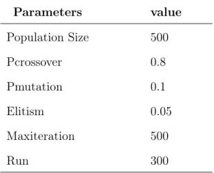
This process of selection, crossover, and mutation repeats for next generations and each time the best solution with the best fitness value is recorded. The process of evolution is continued until the convergence criteria is met. This could be for an algorithm to reach a maximum number of iterations. The process of all the iterations which leads to a value as a solution is called a Run. The second type of convergence occurs when a quite large number of generation passed with almost the same fitness value or without any improvement in it. The third type of convergence is when there is a predefined bound for the population statistic (scrucca2013ga). Performance of a GA depends on the fitness function and parameters like probability of crossover, probability of mutation, size of the population, and the number of iterations which can be adapted after some primary runs (Carr, 2014).

As Carr (2014) explained, Permutation type of Genetic Algorithm is an optimization problem for combinations which means the function is optimized by selecting the best permutation or order of the numbers or items. The very famous problem of permutation type of a GA is "The Traveling Salesman Problem" (TSP).

(37)

2.1

Real-valued GA

When we are interested in optimizing a function, the variables of which are continuous, we are required to apply Real-valued GA. This type of GA is less time consuming since the solutions do not need to be converted to binary values as in the Binary type of GA (Haupt & Haupt, 2004). If the fitness function is bi-variate, f(x, y), with continuous variables x and y, it will report two solutions to the problem. The domain of the variables has to be determined for the function to help GA to limit the search space to a reasonable size (Haupt & Haupt, 2004).

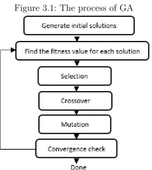
Firstly, the process of optimization of a real-valued GA starts with an initial population of continuous solutions. Secondly, the fitness values of these initial solutions are computed using the fitness function. Then, it will be investigated if they are optimal numbers and the algorithm converges or if they have to be evolved using GA operators through the process of selection, crossover, and mutation. If the initial solutions are not optimal, the second generation of solutions will be produced using the GA operators and the convergence will be checked. This process could continue for several generations until the optimal numbers will be obtained and the GA converges. The whole process of GA which will lead to producing the optimal solutions is depicted in Figure 3.1(see (Haupt & Haupt, 2004)).

Figure 3.1: The process of GA

(38)

used to produce the optimal solutions. Some of the GA operators will be explained in the following sections.

2.2

Selection

The selection process for reproduction is a very crucial step in the optimization of a GA. The selection mechanism determines the individuals that need to be selected to produce the new generation. Also, there is an important parameter in the selection pro-cess called selection pressure which aims for for the selection of the fittest solutions or individuals for producing the next generation. If selection pressure is too low then it slows down the process of convergence to find optimum solutions. If it is too high, the algorithm converges too fast to a local optimum since it does let less fitted solutions to be selected which leads to less diversity in the population. Therefore, it is important to know which selection method to choose that help the algorithm converges to the global optimum solution (Oladele & Sadiku, 2013).

• Roulette Wheel Selection (RWS): Razali, Geraghty, et al. (2011) explained that in this method each individual solution has a probability of being selected proportional to its fitness value. If a solution is denoted by fi, i = 1,2,· · · , n, the probability for a solution to be selected is pi = fi

Pn

i=1fi. In this approach the solution with the highest probability have higher chance of being selected. The process of selection in roulette wheel method can be summarized in these steps:

– S =Pn

i=1fi is the sum of all the fitness values

– α∈(0, S) is a random number generated

– go through the solutions and calculate the sum of fitness values S0 =Pj

i=1fi.

Ifα < S0 then solution j is selected.

– repeat the last two steps to produce enough pairs that could mate and produce new generation or solutions.

For instance, if the current solutions are fi = {1,5,6,7,11,20} and the sum is S = 50 and α is selected randomly from this range α ∈ (0,50) such as α = 23.

(39)

Also, the S0 = 1 + 5 + 6 + 7 + 11 = 30 is computed. since α < S0 then 11 is the one that is selected. This method gives chance to every individual to be selected but the opportunity is not the same for every individual. The ones with the largest probability have more chance to be selected since the selection pressure is too high. They dominate the population and do not let the other individuals to be involved which leads to less diversity in the next generation. Therefore, the algorithm could produce the local optimum rather than global.

• Rank Selection: This method was introduced to bring more diversity to the solutions that cannot be obtained in the previous method due to fittest solutions dominance. In fact this method gives every solution the same chance of being selected. In this method the individuals are ranked according to their fitness values. The individual with the lowest fitness value ranks 1 and the one with the highest fitness value ranks n (Kumar, 2012). Rank selection method prevents the algorithm to converge too fast and will not let the algorithm get stuck in the local optimum. The process of selection in Rank Selection method by considering the rank of a solution as ri can be summarized in these steps (Kumar, 2012):

– S =Pn

i=1ri is the sum of all the fitness values

– α∈(0, S) is a random number generated

– go through the solutions and calculate the sum of fitness values S0 =Pj

i=1ri. Ifα < S0 then the solution j is selected.

– repeat the last two steps to produce enough pairs that could mate and produce new generation or solutions.

For instance, if the current solutions are fi = {1,5,6,7,11,20} and the sum is S = 21and αis selected randomly from this rangeα ∈(0,21) such asα = 14. Also, the S0 = 1 + 2 + 3 + 4 + 5 = 15 is computed. sinceα < S0 then 11is the one that is selected. The problem with this method is that it converges very slowly because it is based on the ranks of the solutions, but it is more robust comparing to the other method of selections. Rank selection method includes two types of methods:

(40)

– Linear Rank Selection: This method was proposed by Blickle and Thiele (1995). In this method the probability of selection is linearly proportional to their rank

pi = 1 n(η − + (η+−η−)i−1 n−1), i∈ {1,2,· · · , n} η+= 2−η−, η−>0 (2.1) In Equation (2.1) the probability of the worst solution to be selected is η_n− and the probability of the best solution to be selected is η_n+. Also, the constraints η+ = 2−η−, η−>0must be achieved as the population size is held invariant. In this method even the individual solutions with the same fitness value get different probability of being selected . In this equation if the fitness value of the fittest individual is set to 2or larger than that, then the worst individual does not have the chance to be selected for the reproduction. By settingη+_>₂_the

worst solutions fitness values will be negative which means they cannot produce any new solutions (Blickle & Thiele, 1995). Another method that gives a chance to the worst members of a population to be selected is the Non-linear Rank selection.

– Non-linear Rank Selection: In this method the probability of selection is not proportional to the rank. it is proportional to a non-linear function of the rank. In this method the selective pressure is higher than linear rank selection, so the algorithm converges slowly to find the optimal solution (Kumar, 2012).

• Linear Scaling Selection(Goldberg & Holland, 1988): This process of selection is defined to overcome the problem of the fittest solutions domination in Roulette wheel selection method. In this method, a linear functionfscaled of the current fitness function fraw is defined as fscaled = afraw+b. The coefficients a and b are selected such that favg

raw = f avg

scaled. Also, fscaledmax =Cfrawavg in which C ∈ (1.1,2) is the number of expected desired copies of best solutions that can be selected to produce the next generation of solutions. In fact, C controls the number of fittest solutions to be selected for the reproduction. The choice of C pulls the fitness function out

(41)

remarkably when the algorithm reaches to the end of the run. This situation causes some problem in using linear scaling. There are some bad solutions with fitness values that are very far from the average and the maximum which are almost close in a mature run. When scaling is applied, since the maximum and average fitness values are so close, it affects the scaled bad fitness values and they become negative. In this case one of the solutions is to map these negative values to zero for the bad fitness values and keep the rest stay the same as they are.

• Sigma Truncation Selection: The previous method works well and prevents the domination of powerful solutions. However, some weak solutions produce negative amounts for the scaled fitness function fscaled due to scaling. In this case, it is sug-gested using the variance of fitness values of the population before scaling. In this process, before scaling a constant is deducted from the raw fitness value and the new fitness function f0 is computed. The new fitness function is f0 =fraw−( ¯f−c×σ) where f¯=Pn

i=1fi and σ is the standard deviation of the fitness values of the pop-ulation. Also, c ∈ (1,3) is selected as a multiple of σ. After sigma truncation is incorporated, and new fitness values f0 are computed, the linear scaling procedure which explained in the previous part can be applied. Sigma truncation prevents from having negative values for scaled fitness values (Goldberg & Holland, 1988).

• Tournament Selection (Jebari & Madiafi, 2013): In this process a subset of the population k < n is selected and from this subset the fittest individual will be the one to be chosen for reproduction. This process repeats n times and for the whole population. Since this method does not involve sorting, it works really well for large populations.

2.3

Crossover

When the parents are selected by one of the methods that described above, then we need to decide how they are going to mate and produce the next generation which leads us to the topic in this section, crossover. There are various methods for crossover which

(42)

was explained by Adewuya (1996):

• Single point crossover: In this method, parents that are selected from the initial population exchange some part of the information to produce the new generation. For instance consider there are k variables involved to the problem that have to be solved. The solution is a k-dimension vector, and the two parents as an example could be F1 = [f1, f2, f3, f4,· · · , fk] and F2 = [f10, f 0 2, f 0 3, f 0 4,· · · , f 0

k]. The new off-spring can be produced by choosing randomly a single point such as point three in the parents and exchange the items between them as follows to produce new solu-tions: F₁new = [f₁0, f₂0, f₃0, f4,· · · , fk] and F2new = [f1, f2, f3, f40,· · · , fk0]. This method is rarely used, and if it is the case, mutation rate has to be high to bring more diversity to the solutions by introducing new members.

• Uniform Crossover: In this method the crossover occurs on multiple points randomly. If two parents are F1 = [f1, f2, f3, f4,· · · , fk] and F2 = [f10, f

0 2, f 0 3, f 0 4,· · · , f 0 k], The new offspring could be produced by choosing randomly a single or multiple points in the parents chromosomes and exchange the items between them as follows F₁new = [f₁0, f2, f30, f4,· · ·, fk]and F2new = [f1, f20, f3, f40,· · · , fk0].

• Local Arithmetic crossover: If F1 and F2 are the parents, the offspring is produced

from these three linear combinations

F₁new = 0.5F1+ 0.5F2 F2new = 1.5F1−0.5F2 F3new =−0.5F1+ 1.5F2

The combinations occurs gene by gene in the parents, and the best two out of these three are selected as the new offspring. This method brings more diversity to the solutions.

• Whole Arithmetic crossover: IfF1andF2are the parents and the offspring is created

through this combination:

(43)

where a∈[0,1]is randomly selected, it is called whole arithmetic crossover.

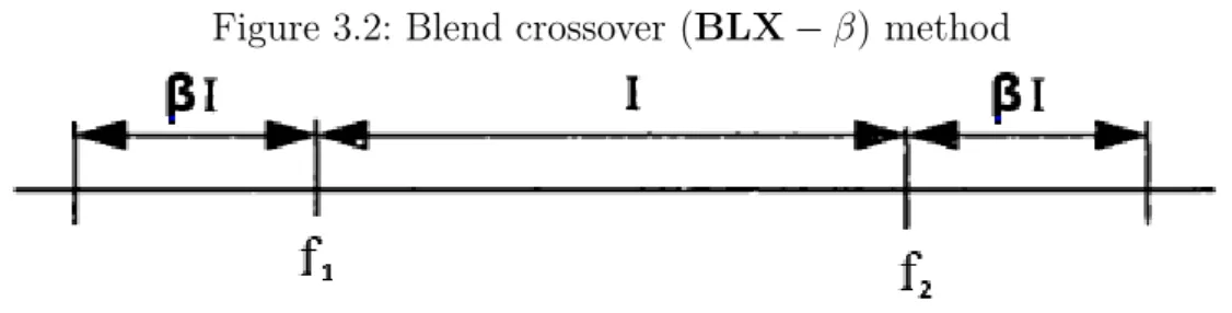
• Blend Crossover (BLX−β): In this method a parameterβis selected that identifies a bound outside the range of values between two parents to produce the new offspring. Figure 3.2 depicts how this type of crossover works:

Figure 3.2: Blend crossover (BLX−β) method

Ifβ = 0 then, it is called flat crossover, and the values are selected from the outside the range of parents values. Parameter β stretches the range of the new generation but not too far.

2.4

Mutation

When the methods for selection and crossover are selected, the next step is to introduce mutation to the algorithm. Mutation brings more diversity to the solutions and also prevents the algorithm from converging too quickly on a local optimum value. There are different methods for mutation as well (Adewuya, 1996):

• Uniform random mutation: If the solution vector for the fitness function and for generation t is Ft _{= (}_f

1, f2,· · · , fj,· · · , fk) and every item has the same chance to be selected, the new solution could beFt+1 _{= (}_f

1, f2,· · · , fj0,· · · , fk)wherefj0, 1≤ j ≤k could be any number between lower and upper bound of thefk. This method produce solutions close to the original solutions.

• Non-uniform random mutation: If the solution vector for the fitness function is Ft= (f1, f2,· · · , fj,· · · , fk)and every item has the same chance to be selected, the

(44)

new solution could be Ft+1 = (f1, f2,· · · , fj0,· · · , fk) where: f_j0 =fj +y×r 1− t T b

where tis the number of current generation, T is the maximum number for genera-tion,r is a random number that is generated and it is between 0 and 1,b determines a non-uniformity is the system parameter, and ytakes values between -1 and 1 with probability of 0.5.

• Random mutation around the solution: If the solution vector for the fitness function is Ft _{= (}_f

1, f2,· · · , fj,· · · , fk) and every item has the same chance to be selected, the new solution could be Ft+1 = (f1, f2,· · · , fj0,· · · , fk) where fj0 could be the lower bound Lj or the upper bound Uj of the fj, 1≤ j ≤k. This method creates solutions with less diversity since the new solution can take values either as the upper or lower bound.

All these methods are the ones that are defined for GA package in R. There are other parameters that have effect on the performance of GA such as probability of crossover, probability of mutation, and elitism. In next section it is discussed how these parameters could have impact on the performance of GA.

2.5

GA control parameters

All the methods that are described above are part of the GA operators: selection, crossover, and mutation. The choice of these methods has effect on the performance of GA. There are also some other parameters which are called control parameters in the GA function that have effect on its performance like population size, probability of crossover, and probability of mutation. Most of the time, the best values for these control parameters are determined by trial and error. There is no single optimal number for these parameters and it changes among various problems or even at different levels of the GA process. He presented some of the studies that investigated the optimal numbers for probability of crossover and probability of mutation (Patil & Pawar, 2015).

(45)

DeJong (1975) explained that high values for the mutation rate decrease the perfor-mance of GA regardless of what values to be assigned to the other parameters. One of their suggestions for these parameters is a population size of (50-100), a single point prob-ability of crossover (0.6) and a probprob-ability of mutation of (0.001) which have been used in many Genetic Algorithms.

Grefenstette (1986) illustr