2016
Topics in empirical Bayesian analysis
Robert Christian Foster
Iowa State University
Follow this and additional works at:
https://lib.dr.iastate.edu/etd
Part of the
Statistics and Probability Commons
This Dissertation is brought to you for free and open access by the Iowa State University Capstones, Theses and Dissertations at Iowa State University Digital Repository. It has been accepted for inclusion in Graduate Theses and Dissertations by an authorized administrator of Iowa State University Digital Repository. For more information, please [email protected].
Recommended Citation
Foster, Robert Christian, "Topics in empirical Bayesian analysis" (2016).Graduate Theses and Dissertations. 15910.
by
Robert Christian Foster
A dissertation submitted to the graduate faculty in partial fulfillment of the requirements for the degree of
DOCTOR OF PHILOSOPHY
Major: Statistics
Program of Study Committee: Mark Kaiser, Major Professor
Petrut¸a Caragea Daniel Nettleton
Jarad Niemi Daniel Nordman
Iowa State University Ames, Iowa
2016
DEDICATION
I would like to dedicate this dissertation to my mother, without whose constant love and support I would not have been able to complete it.
TABLE OF CONTENTS
LIST OF TABLES . . . vi
LIST OF FIGURES . . . ix
ACKNOWLEDGEMENTS . . . x
ABSTRACT . . . xi
CHAPTER 1. INTRODUCTION AND OUTLINE . . . 1
1.1 Bayesian and Empirical Bayesian Methods . . . 1
1.2 Dissertation Organization . . . 1
CHAPTER 2. EMPIRICAL BAYESIAN INTERVAL WIDTHS . . . 3
2.1 Introduction and Literature Review . . . 3
2.1.1 Modern Empirical Bayes . . . 3
2.1.2 Corrected Intervals . . . 5
2.1.3 Bias-Corrected Intervals . . . 5
2.1.4 Morris Intervals . . . 7
2.1.5 Bootstrap Approach . . . 8
2.1.6 Hyperprior Approach . . . 9
2.2 The Empirical Bayes Problem for the Beta-Binomial Model . . . 10
2.2.1 The Beta-Binomial Model . . . 10
2.2.2 Beta-Binomial Model Formulation and Estimation Form . . . 11
2.2.3 Framework for Comparison . . . 12
2.2.4 Additional Framework . . . 13
2.3 Analysis . . . 14
2.3.1 Interval Widths . . . 14
2.3.3 Practical Example . . . 15 2.3.4 Explanation . . . 17 2.3.5 KnownM . . . 19 2.3.6 Simulation Study . . . 20 2.3.7 Analysis of Phenomenon . . . 23 2.3.8 Non-Bayesian Methods . . . 27 2.3.9 Unknown M . . . 28 2.3.10 Further Simulations . . . 30 2.3.11 Recommendations . . . 31 2.4 Future Work . . . 32 2.5 Conclusion . . . 32
CHAPTER 3. COMPARISON FRAMEWORK FOR THE NATURAL EX-PONENTIAL FAMILY WITH QUADRATIC VARIANCE FUNCTIONS 34 3.1 NEFQVF Families . . . 34
3.1.1 NEFQVF Distributions . . . 34
3.1.2 NEFQVF Shrinkage . . . 35
3.1.3 Morris Hyperpriors . . . 37
3.2 Interval Comparison Framework . . . 40
3.2.1 The Gamma-Poisson Model . . . 41
3.2.2 Interval Width Comparison . . . 42
3.2.3 Simulated Data . . . 43
3.3 Corrected Intervals . . . 45
3.4 Conclusion . . . 48
CHAPTER 4. BAYESIAN AND EMPIRICAL BAYESIAN ESTIMATION OF A BASEBALL TEAM’S WINNING PERCENTAGE USING THE ZERO-INFLATED GEOMETRIC DISTRIBUTION . . . 50
4.1 Winning Percentage Estimators . . . 50
4.3 Winning Percentage Estimator . . . 52
4.4 Model Fit . . . 53
4.5 Comparisons . . . 55
4.6 Interval Estimation . . . 58
4.7 An Empirical Bayesian Approach to Estimation . . . 61
4.8 Conclusion and Further Work . . . 64
BIBLIOGRAPHY . . . 65
APPENDIX A. ESTIMATION PROCEDURES . . . 68
APPENDIX B. TERBINAFINE DATA AND ANALYSIS . . . 70
APPENDIX C. SIMULATIONS (KNOWN M) . . . 73
APPENDIX D. SIMULATIONS (UNKNOWN M) . . . 78
LIST OF TABLES
Table 2.1 Selected Empirical Bayesian and Hierarchical Bayesian Estimates for Terbinafine Trials . . . 16
Table 2.2 Selected Empirical Bayesian and Hierarchical Bayesian Interval Widths for Terbinafine Trials . . . 17
Table 2.3 Empirical and Hierarchical Bayesian Interval Widths and Coverage -µ= 0.10,Known M = 4, ni =k= 10 . . . 21
Table 2.4 Non-Bayesian Correction Methods Coverage and Interval Width —µ= 0.1,Known M = 4, k=ni= 10 . . . 28
Table 2.5 Empirical and Hierarchical Bayesian Interval Widths and Coverage -µ= 0.10, M = 4, ni=k= 10 . . . 30
Table 2.6 Non-Bayesian Correction Methods Coverage and Interval Width —µ= 0.1, M = 4, k=ni= 10 . . . 31
Table 3.1 Empirical and Hierarchical Bayesian Interval Widths and Coverage -µ= 0.10,Known M = 4, ni =k= 10 . . . 44
Table 3.2 Naive MLE EB (Left) and Morris Corrected EB (Right) Interval Widths and Coverages for the Gamma-Poisson Model . . . 46
Table 3.3 Naive MLE EB (Left) and Morris Corrected EB (Right) Interval Widths and Coverages for the Beta-Binomial Model . . . 48
Table 4.1 Empirical and Zero-Inflated Geometric Distributions of Runs Scored per Inning for the 2015 Atlanta Braves . . . 54
Table 4.2 Empirical and Zero-Inflated Geometric Distributions of Runs Allowed per Inning for the 2015 Atlanta Braves . . . 54
Table 4.3 Observed Wins, Pythagorean Expectation (P.rean), Pythagenpat Ex-pcectation (P.pat), and Zero-Inflated Win Probability (ZI) for the 2015 MLB Season . . . 55
Table 4.4 Mean squared errors for all baseball teams for the pythagorean, pytha-genpat, and zero-inflated geometric winning percentage estimation tech-niques from 2000 to 2015 . . . 57
Table 4.5 95% Maximum Likelihood and Central Bayesian Intervals for the Win-ning Total of MLB Teams in the 2015 Season . . . 60
Table B.1 Terbinafine Trials Data and Raw Adverse Reaction Proportion . . . . 70
Table B.2 Terbinafine Trials Empirical and Hierarchical Bayesian Estimates . . . 71
Table B.3 Terbinafine Trials Empirical and Hierarchical Bayesian Interval Widths 72
Table C.1 Empirical and Hierarchical Bayesian Interval Widths and Coverage -µ= 0.50,Known M = 4, ni =k= 10 . . . 73
Table C.2 Non-Bayesian Correction Methods Coverage and Interval Width —µ= 0.5,Known M = 4, k=ni= 10 . . . 74
Table C.3 Empirical and Hierarchical Bayesian Interval Widths and Coverage -µ= 0.10,Known M = 100, ni=k= 10 . . . 75
Table C.4 Non-Bayesian Correction Methods Coverage and Interval Width —µ= 0.1,Known M = 100, k=ni = 10 . . . 75
Table C.5 Empirical and Hierarchical Bayesian Interval Widths and Coverage -µ= 0.10,Known M = 4, ni =k= 30 . . . 76
Table C.6 Non-Bayesian Correction Methods Coverage and Interval Width -µ= 0.1,Known M = 4, k=ni= 30 . . . 77
Table D.1 Empirical and Hierarchical Bayesian Interval Widths and Coverage -µ= 0.50, M = 4, ni=k= 10 . . . 78
Table D.2 Non-Bayesian Correction Methods Coverage and Interval Width -µ= 0.5, M = 4, k=ni= 10 . . . 79
Table D.3 Empirical and Hierarchical Bayesian Interval Widths and Coverage -µ= 0.10, M = 100, ni =k= 10 . . . 79
Table D.4 Non-Bayesian Correction Methods Coverage and Interval Width -µ= 0.1, M = 100, k=ni= 10 . . . 80
Table D.5 Empirical and Hierarchical Bayesian Interval Widths and Coverage -µ= 0.10, M = 4, ni=k= 30 . . . 80
Table D.6 Non-Bayesian Correction Methods Coverage and Interval Width -µ= 0.1, M = 4, k=ni= 30 . . . 81
LIST OF FIGURES
Figure 2.1 Empirical Bayesian Posterior Distributions for Adverse Reaction Pro-portion of Arm 19 of Terbinafine Trials . . . 18
Figure 2.2 Ratio of Empirical Bayesian Interval Widths by Method of Moments to Hierarchical Bayesian Interval Widths by Haldane’s Prior . . . 22
Figure 2.3 Ratio of Empirical Bayesian Interval Width using Method of Moments over Average (Within Data Set) Hierarchical Bayesian Interval width using Haldane’s Prior versus Ratio of ˆµEstimates (Method of Moments Over Maximum Likelihood) foryi = 0 . . . 26
Figure 2.4 Ratio of Empirical Bayesian Interval Width using Method of Moments over Average (Within Data Set) Hierarchical Bayesian Interval width using Haldane’s Prior versus Ratio of ˆµEstimates (Method of Moments Over Maximum Likelihood) foryi = 1 . . . 27
Figure 3.1 Ratio of Method of Moments Empirical Bayesian Interval Width to Mor-ris Hyperprior Bayesian Interval Width by Ratio of ˆµM M over ˆµM LE,
ACKNOWLEDGEMENTS
I would like to thank all my friends that supported me throughout graduate school — Danielle and Jonathan, Dan F., Brian, Dan A. and Julie, Laura, Lisa, Marcela, Kristian and Chris, and Adam and Arielle. Without their support I likely would not have completed this dissertation.
I would also like to thank the department of statistics at Iowa State University for continuing to support me, though I was not always the ideal student.
I would like to thank my committee of Dr. Jarad Niemi, Dr. Daniel Nettleton, Dr. Daniel Nordman, and Dr. Petrut¸a Caragea for their patience in working with me.
Lastly, I would like to thank my Dr. Kaiser for all the illuminating talks that we have had in the process of creating this dissertation, and for the many helpful comments and suggestions he has given.
ABSTRACT
While very useful in the realm of decision theory, it is widely understood that when ap-plied to interval estimation, empirical Bayesian estimation techniques produce intervals with an incorrect width due to the failure to incorporate uncertainty in the estimates of the prior parameters. Traditionally, interval widths have been seen as too short. Various methods have been proposed to address this, with most focusing on the normal model as an application and many attempting to recreate, either naturally or artificially, a hierarchical Bayesian solution. An alternative framework for analysis in the non-normal scenario is proposed and, for the beta-binomial model, it is shown that under this framework the full hierarchical method may produce interval widths that are shorter than empirical Bayesian interval widths. Furthermore, this paper will compare interval widths and frequentist coverage for different Bayesian and non-Bayesian interval correction methods and offer recommendations. This framework may also be extended to the larger natural exponential family with quadratic variance functions, of which the beta-binomial model is a member, and general properties of NEFQVF distributions are given, with a specific application of the gamma-Poisson model. A class of prior is introduced as a limiting state of the framework that, in the hierarchical setting where the shrinkage co-efficient is known, extends the well-known conjugacy of NEFQVF families to the hierarchical setting in an approximate way, and intervals are constructed using a refined empirical Bayesian interval correction technique that produce an alternative comparison basis. Coverage and in-terval widths are shown for this technique for the beta-binomial and gamma-Poisson models. Both produce near-nominal coverage and compare favorably to the full hierarchical solution calculated using MCMC.
As a second topic, a new Bayesian and empirical Bayesian estimate of a baseball team’s “true” winning percentage is introduced. Common methods for estimating this “true” winning percentage, such as the pythagorean expectation or pythagenpat system, rely on the total
number of runs scored and allowed over a period of time. A new estimator is proposed that uses independent zero-inflated geometric distributions for runs scored and allowed per inning to determine a winning percentage. This estimator outperforms methods based on total runs scored and allowed in terms of mean-squared error using actual win totals. Interval estimation for this estimator is directly shown using frequentist or Bayesian techniques. Empirical Bayesian techniques are shown as an approximation to the full hierarchical solution. Selected interval widths are compared using all three methods, with slight differences in the shrinkage amount given a full season’s worth of data.
CHAPTER 1. INTRODUCTION AND OUTLINE
1.1 Bayesian and Empirical Bayesian Methods
Bayesian and empirical Bayesian methods have found a wide use within statistical prac-tice. Modern usage of empirical Bayesian methodologies has ranged from small-area estimation problems to large sample analysis of microarray data, while traditional Bayesian methods have expanded into a rich practice in hierarchical modeling. This dissertation presents new research within the field of empirical Bayesian estimation and its connection to Bayesian estimation and frequentist estimation. Three separate applications of Bayesian and empirical Bayesian methodologies are introduced, focusing on practice, theory, and application.
1.2 Dissertation Organization
In the first chapter, focusing on practice, a brief literature review discusses various methods of correcting the widths of empirical Bayesian intervals, with the implied reasoning of the correc-tion method as to the correct basis of comparison indicated. A new framework is introduced for the beta-binomial model that provides an intermediate stage between empirical Bayesian and hierarchical Bayesian methods which matches expectations of prior distributions to estimates of prior distributions, and some properties are shown that connect this framework to some of the given correction techniques. A specific application using medical data is shown in which empirical Bayesian interval widths exceed those of a “noninformative” hierarchical Bayesian analysis, and it is further shown that in this framework, it is entirely reasonable that an em-pirical Bayesian interval width may exceed a hierarchical Bayesian interval width. Simulations are conducted to determine what types of data sets are likely to have this phenomenon present itself, and to compare the properties of the intermediate priors and full hierarchical priors to
the non-hierarchical correction methods for both known and unknown shrinkage amounts, with generally positive results.
In the second chapter, focusing on theory, the ideas from the first chapter are extended to the natural exponential family with quadratic variance function (whose properties are briefly reviewed), and a general form of the framework from the first chapter is introduced in the case with known shrinkage amount. Taking the limiting case of this framework leads to a class of hyperpriors which, in the case of known shrinkage amount, produce a form of strong approximate conjugacy for hierarchical models, and which may be used as a basis for comparison of empirical Bayesian interval widths in some scenarios. A specific case of the gamma-Poisson model is shown, and simulated data shows empirical Bayesian interval widths that exceed hierarchical Bayesian interval widths. Finally, the strong approximate conjugacy property is used to refine a method for correction of empirical Bayesian intervals widths described in Morris (1988), and simulations show the refined method performs well in terms of coverage and interval length, with results close to those of the full hierarchical model.
Lastly, an application of Bayesian and empirical Bayesian methodologies is given. A class of winning percentage estimators for baseball teams is briefly reviewed, along with efforts of modeling run scoring distributions, and a new estimator is introduced that relies on parametric modeling of run scored and allowed distributions with a zero-inflated geometric distributions. This winning estimator compares well to the existing estimators when fit using maximum likelihood techniques in terms of root mean squared difference from the actual win totals, and interval estimation (generally not attempted for winning percentage estimators) is shown using maximum likelihood and Bayesian estimation. Empirical Bayesian estimation is shown as an alternative to the full hierarchical Bayesian model, and offers a computationally simpler analysis.
CHAPTER 2. EMPIRICAL BAYESIAN INTERVAL WIDTHS
2.1 Introduction and Literature Review
The idea of “empirical Bayes” is not a precisely defined concept within modern statistics. Some consider it a specific technique, others consider it a class of techniques, and yet others consider it to be a philosophical approach to data analysis. Generally the idea revolves around empirical bayes as a sort of “pseudo-Bayes” — a way to, as Carlin and Louis (2000) state, “compromise between the frequentist and Bayesian methods.”
Though more commonly viewed through a decision-theoretic framework, intervals may be based on empirical Bayesian estimates. Conventional wisdom states that these intervals are necessarily too narrow due to underestimation of the variance; however, these comparisons are often based upon idealized scenarios, and usually only the Gaussian-Gaussian model.
2.1.1 Modern Empirical Bayes
The dual work of Herbert Robbins and Carl Morris & Brad Efron has led to the development of two branches of empirical Bayes theory. The first, nonparametric empirical Bayess, follows in the Robbins tradition of assuming that a common prior G(.) exists, but the form is unknown, and so inference proceeds based off of the marginal density. The second branch, known as parametric empirical Bayes, builds off of Morris and Efron’s 1975 work connecting Stein’s estimator to Bayesian procedures. Parametric empirical Bayes will be the focus of this article. The parametric empirical Bayes model will be as follows: suppose there are observations y1, ..., yk (note that yi may be a vector or a sufficient statistic) from some parametric density
use Bayes’ rule to derive the posterior distributions and an estimates for the θi. In parametric
empirical Bayes, however, a prior distributionG(θi|η) indexed by some parameterηis used (and
note thatη may be a vector). An estimate ˆη is provided by the marginal densitymG(yi|η) =
R
f(yi|θi)G(θi|η)dθi, usually through a common estimation procedure such as the method of
moments or the method of maximum likelihood, and the posterior distributions for θi are
derived usingG(θi|ηˆ) as a common prior.
The problem is formulated as
y1, y2, ..., yk indep ∼ f(yi|θi) θi iid ∼G(θi|ηˆ) (2.1)
When working in an ideal empirical Bayesian setting (such as the Gaussian/Gaussian model), a 95% empirical Bayesian confidence interval might be given by
E[θi|yi,ηˆ]±1.96
p
V ar(θi|yi,ηˆ) (2.2)
It is commonly understood, however, that this is “naive” in the sense that it does not incorporate uncertainty in the estimated parameter or parameters ˆη of the prior distribution. Under the parametric empirical bayes model, a standard two-stage variance decomposition of V ar(θi|y) is given by
V ar(θi|yi) =Eη|yi[V ar(θi|yi, η)] +V arη|yi[E(θi|yi, η)] (2.3)
Carlin and Louis (2000) note that the quantity pV ar(θi|yi,ηˆ) in equation (2.2)
approxi-mates the first term — it does not, however, address the second term in equation (2.3), which Carlin and Louis (2000) identify as “the posterior uncertainty aboutη.”
In the non-Gaussian setting, where the posterior distribution is not symmetric, intervals for the parametersθi may be produced through quantiles of the posterior distribution forθi —
and though not taking the same form, share the same issue of not accounting for the posterior uncertainty regarding ˆη.
2.1.2 Corrected Intervals
In order to accurately assess the confidence level, a precise notion of “confidence” for em-pirical Bayes intervals must first be constructed. Carlin and Gelfand (1991) define tα(y) as a
(1−α)×100% confidence interval for θi if
Pη(θi∈tα(y))≈1−α (2.4)
Morris (1983a) has a similar definition, but with ≥1−α. Carlin and Louis (2000) refer to this type of interval as an unconditional confidence interval — that is, it requires confidence over the variation in both the θi and the datay.
Carlin and Gelfand (1991) note that some consider this statement weak, and suggest that “a probability statement which offers conditional calibration given an appropriate data summary” would likely be preferred. They define an alternative interval as tα(y) to be a (1−α)×100%
confidence interval forθi if
P(θi ∈tα(y)|b(y) =b)≈1−α (2.5)
where b(y) is an appropriate summary statistic of y (even up to taking b(y) = yi). This is
known as a conditional empirical bayes confidence interval, since it requires confidence strictly over the variation in the θi. Essentially, demanding conditional coverage requires that given
an appropriate summary statistic, any set of empirical Bayesian intervals calculated from that statistic has nominal coverage, while demanding unconditional coverage allows the conditional coverage given each summary statistic to vary so long as the coverage over all possible summary statistics is nominal. This paper will focus on estimating unconditional coverage. Multiple pro-cedures have been proposed to adjust the coverage so as to reach nominal coverage rates.
2.1.3 Bias-Corrected Intervals
One approach to producing “correct” intervals — and one of the few not mimicking a hyperprior solution — is found in Efron’s comments on Laird and Louis (1987) and further
explained in Carlin and Gelfand (1990), as a method to conditionally correct the bias from the empirical Bayes procedure.
Taking the general empirical Bayes setup as described in equations (2.1) but first supposing that there exists a true value of η which is known, empirical Bayes confidence intervals are calculated by first taking quantiles from the posterior density of theθi:
(qα/2(yi, η), q1−α/2(yi, η))
whereqα(yi, η) is defined by
P(θi≤qα(yi, η)|θi ∼p(θi|yi, η)) =α
That is, they are the posterior quantiles from the posterior distribution that uses the true value of η. Of course, in practice the true value of η is unknown and must be estimated with ˆ
η — it is then possible to define
r(ˆη, η, yi, α) =P(θi≤qα(yi,ηˆ)|θi∼p(θi|yi, η))
That is, the probability thatθi (on the true posterior usingη) is less than sample quantile
taken from the estimated posterior using ˆη. Since ˆη is random, the expected probability can be taken
R(η, yi, α) =Eηˆ|yi,η[r(ˆη, η, yi, α)] (2.6)
This is the average probability (over ˆη) thatθi is less than the sample quantile taken from
the estimated posterior using ˆη with lower probability α. The expectation in equation (2.6) does not actually have to be close to the nominalα. However, it is possible to solve
R(η, yi, α0) =α
forα0 — that is, there exists a nominal valueα0 that, when used to take sample quantiles, pro-duces expected lower probabilityαon the true posterior. Using α0 when taking quantiles from the empirical Bayesian posterior, then, could correct for the underestimation of the variance.
In practice, however, η is not know, so instead the estimate ˆη is treated as the true value, and the quantity
R(ˆη, yi, α0) =α
is solved forα0. Again, using α0 in place of α when taking quantiles from the posterior distri-bution for θi can be used to correct for the underestimation of the variance.
In the idealized normal-normal scenario, this correction can be calculated analytically. In other situations, it may have to be solved numerically, or a bootstrap method may be used to solve the unknown quantities. Theoretical details may be found in Carlin and Gelfand (1990) and practical implementation through a bootstrap approach may be found in Carlin and Gelfand (1991).
2.1.4 Morris Intervals
Most correction approaches attempt to place or mimic the results of a full hyperprior h(η) on η. In Morris (1983b), Carl Morris uses a model with yi ∼ N(θi, σ2) (σ2 known) and
θi ∼N(µ, A) with a flat improper prior on µand a U nif[0,∞) prior on A to derive intervals
based on the full hierarchical Bayesian procedure. These intervals are centered around the empirical Bayesian estimate
ˆ
θi = (1−Bˆ)yi+ ˆBy¯
Calculations for the posterior variance are complicated and do not extend well to the case with non-constant varianceσ2i, so Morris (1983c) proposes an approximation by
ˆ θi±zα/2 s σ2 1−k−1 k ˆ B + 2 k−3 ˆ B2(y i−y¯)2 where ˆ B= (k−3)σ 2 P (yi−y¯)2
Based on simulations in Carlin and Louis (2000), Morris’s method produces empirical Bayes intervals that achieve or exceed the nominal 95% level in the normal situation, with a width that is shorter than the hierarchical Bayesian method. However, this formula is based explicitly on the assumption of a normal-normal model. Similar intervals are discussed in Efron (2010). Morris extended the idea, if not the same equational form, of hierarchical Bayesian calcu-lations in Morris (1988) to apply to empirical Bayes estimators when working with the natural exponential family with quadratic variance function, using a naive, moment-based estimator for η and using edgeworth expansions to account for sources of uncertainty. In the case of the normal distribution, this method worked very well and holds the standard 95% confidence property. For non-normal data, or for confidence intervals derived instead from quantiles of the posterior distribution of empirical Bayes, it is uncertain if the properties also hold, and Morris suggested that such can only be checked by Monte-Carlo techniques. In addition, Morris’s technique assumes ni = n for all i, and this is admittedly uncommon in most applications.
This would complicate his analysis in the normal case, and moreso in the non-normal case.
2.1.5 Bootstrap Approach
More commonly, the prior is estimated by bootstrap methodology. Laird and Louis (1987) discuss three types of bootstrap samples, with classification depending on assumed knowledge of the forms off(yi|θi) andG(θ|ηˆ). For the third type of bootstrap — which fits the parametric
empirical Bayesian framework and will be used in this paper — a sample θ∗ is produced from G(θ|ηˆ), which is subsequently used to produce a sample from the distribution f(yi|θi∗). An
estimate η∗ is then calculated using the same techniques used on the marginal distribution mG(yi|η) as before. For any of the bootstrap sampling techniques, intervals can then be
cal-culated by mimicking the hyperprior distribution calculation — in particular, forN bootstrap samples, define fG∗(θi|yi,ηˆ) = 1 N N X j=1 fG(θi|yi, ηj∗)
whereη∗ is the estimated value ofη for each bootstrap sample andfG(θi|yi, η) is the posterior
distribution ofθi given datayi and prior parametersη. The distributionfG∗(θi|yi,ηˆ) represents
an artificially created posterior distribution forθi (centered around the same value as the
non-bootstrapped estimate) incorporating the uncertainty in ˆηestimated by the bootstrap method. Equal-tailed confidence intervals forθi can then be found by solving
α 2 = Z CL −∞ fG∗(θ|yi,ηˆ) = Z ∞ CU fG∗(θ|yi,ηˆ)
This often must be calculated numerically, although in the normal-normal case the third type of bootstrap interval is equivalent to a flat hyperprior on η when the prior variance is known. In the normal-normal case with unknown prior variance, the bootstrap posterior can not match a hyperprior Bayesian posterior. Simulation results show that the third type of bootstrap intervals compare very well to the naive bootstrap intervals.
2.1.6 Hyperprior Approach
Another approach is proposed by Deely and Lindley (1991). Known as “Bayes empirical Bayes”, a clever sequence of substitutions and applications of Bayes rule is used to determine that for a given hyperpriorh(η), the posterior distribution of θi independent of η may be
cal-culated as p(θi|y) = R p(θi|yi, η)Qki=1mG(yi|η)h(η)dη R Qk i=1mG(yi|η)h(η)dη
Though equation (2.1.6) is usually not numerically tractable, derivations of forms for the ex-ponential family are given by Deeley and Lindley, and an example is given using an exex-ponential- exponential-Poisson model with an improper hyperprior on η. Quantiles could be taken from this density to form an interval. Walter and Hamedani (1987) give a form of Bayes empirical Bayes estima-tion for a binomial probability using orthogonal polynomials and Walter and Hamedani (1991) extend this approach to the natural exponential family with quadratic variance functions.
One key difference in the theoretic formulation between the Morris and bootstrap methods and the Bayes empirical Bayes method is that the Morris and bootstrap methods essentially treat the empirical Bayesian estimates as correct and attempt to adjust the posterior distribu-tion around them to achieve nominal coverage. No claim is made, however, that the posterior means of the Bayes empirical Bayes densities matches the empirical Bayes posterior means. This subtle difference belies a fundamentally different approach to the connection between empirical and full Bayesian methodologies.
2.2 The Empirical Bayes Problem for the Beta-Binomial Model 2.2.1 The Beta-Binomial Model
Historically, the development of parametric empirical Bayesian methods, including correc-tion methods discussed in Seccorrec-tion2.1, has focused upon the normal-normal model, and results derived apply well to that scenario. This is particularly true in the area of interval estimation, where, apart from positive-part corrections, likelihood estimates are functions of basic mo-ments, and prior distributions that yield hierarchical Bayesian estimates which are equivalent to the empirical Bayesian estimates exist and can be determined.
Less effort has been expended on the application of the previous techniques to models other than the normal-normal; or, if they are mentioned, it is only as a theoretical application of the technique that is not studied — Carlin and Gelfand (1991) gives technical details for parametric bootstrap estimation of the bias correction method applied to the beta-binomial model without providing a specific example or study to illustrate the method.
Empirical Bayesian methodologies are applicable in this situation, and in fact, the original example showing the effectiveness of empirical Bayesian methods in Efron and Morris (1975) was predicting baseball batting averages after transformation so that the normal-normal model could be applied. For the normal-normal model, the idea that a simple widening of the empirical Bayesian corrects the empirical Bayesian problem of uncertainty in the hyperprior parameters is taken as a given. Whether this issue can also be taken for granted in a non-normal scenario, and whether correction methods are necessary, has generally not been investigated.
2.2.2 Beta-Binomial Model Formulation and Estimation Form
The beta-binomial model is now considered:
yi|θi indep
∼ Bin(θi, ni)
θiiid∼Beta(µ, M)
(2.7)
for i = 1,2, ..., k. In place of the traditional α, β parametrization, the transformation µ = α/(α+β) andM =α+β will be applied, representing the mean of the beta distribution and a parameter that controls (but is not equal to) the variance, respectively —M will be referred to as a “variance parameter.” All beta distributions will be defined in terms ofµand M unless otherwise noted. This parametrization of the beta distribution then has mean and variance
E[θi] =µ
V ar(θi) =
µ(1−µ) M+ 1
An alternative parametrization that will be used when M is unknown is
θi ∼Beta0(µ, φ) (2.8)
where µ is as before and φ = 1/(α+β + 1) = 1/(M + 1) is the dispersion parameter of the beta distribution. In this paper, the Beta0(µ, φ) distribution with φis used only for modeling purposes and no priors are defined using this parametrization.
A simple Bayesian analysis would choose values for µ and M (for example, µ = 0.5 and M = 1 yields the Jeffrey’s prior) and proceed using the well-known conjugacy of the beta prior for the binomial distribution. The form of the Bayesian estimator given by the expectation of the resulting posterior is then
ˆ θ=µ+ 1− M M+ni yi ni −µ (2.9) The empirical Bayesian method would be to estimate the parameters µ and M by some method, such as the method of moments or marginal maximum likelihood, and use equation (2.9) above with ˆµand ˆM in place of µand M. The empirical Bayesian estimator is then
ˆ θ= ˆµ+ 1− Mˆ ˆ M+ni ! yi ni −µˆ (2.10)
Intervals may be constructed by drawing quantiles from the posterior distribution for θi
(qα/2(yi,µ,ˆ Mˆ), q1−α/2(yi,µ,ˆ Mˆ))
Another option is to perform a full hierarchical Bayesian analysis by choosing hyperpriors for the parameters µ and M (or equivalently φ) and conducting the full analysis through Markov-Chain Monte Carlo techniques, though technical details of the MCMC procedure will not be covered here. The resulting ˆθ estimates can not, in general, be calculated as solutions of closed-form equations.
2.2.3 Framework for Comparison
The traditional folklore of empirical Bayesian analysis is that it underestimates the variance by using the data twice, and underestimation of the variance takes the form of the standard two-stage variance decomposition in equation (2.3). In addressing this, there generally has been only one methodology — that of Morris (1983b) which considers the appropriate correction to be that obtained through a fully Bayesian analysis with a prior distribution such that
E[θi|yi]≈θˆiEB
where ˆθiEB is given by standard empirical Bayesian estimators, as in equation (2.2.2). Here,
the posterior expectation of the fully Bayesian procedure yields the same expected value as the empirical Bayesian estimators — the exception being the “Bayes empirical Bayes” analysis of Deely and Lindley (1991), which gives an example of computing posterior expectations in exponential families with very specific priors and hyperpriors.
2.2.4 Additional Framework
The Morris-type framework is particularly appealing in that it does not require the com-parison of differences in posterior estimates caused by differences in priors; rather, it considers the empirical Bayes estimates as “correct” and defines the true interval width to be the inter-val width resulting from a full Bayesian analysis that produces those estimates. Furthermore, there is no need to compare different estimation techniques as there is, essentially, only one estimator.
This paper will propose and investigate additional frameworks more similar to the frame-work of Deeley and Lindely — first, rather than matching empirical Bayesian estimates of θi
to posterior Bayesian estimates of the θi, one may match estimates ˆµand/or ˆM to the means
of hyperprior distributions in a hierarchical Bayesian analysis. In this way, the full prior on the θi given by integrating out over the priors at each stage will have expected value matching the
expected value of the empirical Bayesian prior distributions — and so the interval widths may be compared to a full Bayesian analysis with a sufficiently diffused prior rather than posterior. This has the added benefit of using proper prior distributions, although this method, similarly to the Bayes empirical Bayes method of Deely and Lindley (1991), will not necessarily lead to posterior θi estimates that are equivalent to empirical Bayesian estimates.
In the general hierarchical Bayesian setting, this will be proposed as
yi indep ∼ f(yi|θi) θiiid∼G(θi|η) η∼h(η|ηˆ) (2.11)
where ˆηis the estimate used in the empirical Bayesian analysis. As an example, in the normal-normal scenario with known prior variance τ2, this would be proposed as
yi indep ∼ N(θi, σ2) θi iid ∼N(µ, τ2) µ∼N(ˆµ, τ02)
The empirical Bayesian estimator may then be constructed as the resulting posterior taking the hyperprior varianceτ2
0 to zero and creating a degenerate distribution at ˆµwith probability
one, and the flat hyperpriorh(µ)∝1 that Morris (1983b) uses to produce interval corrections can be created by taking the un-normalized density as τ02 approaches infinity.
Aside from producing an intermediate connection between empirical and hierarchical Bayesian estimates, the necessity of this is that in models other than the normal-normal, there may exist multiple methods to estimate the parameters of the prior distribution — and not all of these methods will have an extant prior that yields posterior expectations equal to empirical Bayes estimates without using a highly informative prior. One may be approximated using the boot-strap method of Laird and Louis (1987), but there’s no reason to suggest that this is necessarily the correct thing to do or that it is the only possible choice for comparison — there may exist a hierarchical Bayesian prior yielding nominal frequentist coverage with shorter intervals.
As data for comparison, two different sources will be used:
1. Existing data that has been analyzed with empirical Bayesian techniques 2. Data randomly generated from a beta-binomial model
Coverage assessments are possible for the second data source, and interval widths may be contrasted between empirical Bayesian and hierarchical Bayesian methodologies for both data sources.
2.3 Analysis 2.3.1 Interval Widths
A key question that illustrates the inadequacy of the current comparison framework is whether it is possible under reasonable circumstances to have an empirical Bayesian interval that is, in fact, wider than the hierarchical Bayesian width and if so, by how much. This is an issue generally not considered under the idealized normal-normal model, as the corrected posterior retains the traditional bell shape, but with an increased posterior variance. However, it is an issue that can occur for the beta-binomial model under the proposed framework, and
particularly occurs due to the presence of several consistent estimators for the parameters µ and M of the underlying beta distribution.
2.3.2 Estimation Procedures
The two procedures considered for estimation of the parameters in the beta-binomial model are the method of moments and the method of maximum likelihood. Both procedures were applied to the marginal density of the beta-binomial model, more commonly known as the beta-binomial distribution. For method of moments, both a “naive” method that only requires plugging in of values and a more sophisticated moments procedure that takes an iteratively weighted average were considered. Details of the estimation procedures may be found in Ap-pendix A.
When all binomial sample sizes are equal (the case that will typically be addressed in this paper), the naive moments estimator produces the same estimates as the iterated moments estimator, and will simply be referred to as the method of moments estimate. When sample sizes differ, the iterated moments estimator produces estimates that tend to be closer in value to the estimates produced by maximum likelihood.
2.3.3 Practical Example
The method used for prior estimation can and will affect resulting interval widths - an example comes from Young-Xu and Chan (2008). In trials of antifungal medicine terbinafine, N = 41 treatments arms were considered. The responseyi in arm iis the number of patients
(out ofnitotal) that withdrew from the trial due to adverse reactions to the medication. These
data are presented in TableB.1 in AppendixB.
Empirical Bayesian estimates and intervals were calculated using the naive method of mo-ments, an iteratively weighted method of momo-ments, the method of maximum likelihood, and a Bayesian procedure with priors
p(µ)∝ 1
µ(1−µ) φ∼Beta(0.5,1)
where φ is as in equation (2.8). The full set of Bayesian priors was chosen to represent a noninformative Bayesian solution.
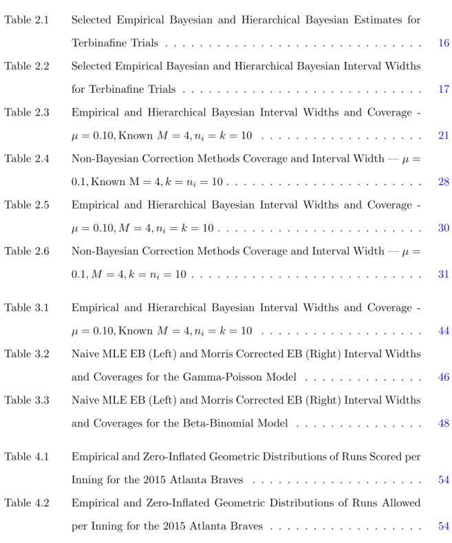
Selected empirical Bayesian estimates using a naive unweighted method of moments (NMM), iterated method of moments (IMM), maximum likelihood (MLE), and full hierarchical Bayesian (HB) estimates, rounded to three decimal places, are given below in Table 2.1. The full table is given in AppendixB.
Table 2.1 Selected Empirical Bayesian and Hierarchical Bayesian Estimates for Terbinafine Trials Arm θˆi N M M ˆ θi IM M ˆ θi M LE ˆ θi HB Arm θˆi N M M ˆ θi IM M ˆ θi M LE ˆ θi HB 1 0.038 0.037 0.037 0.038 21 0.023 0.019 0.018 0.018 5 0.029 0.023 0.021 0.020 25 0.024 0.017 0.014 0.014 10 0.060 0.068 0.073 0.074 30 0.030 0.026 0.024 0.024 15 0.031 0.026 0.024 0.023 35 0.019 0.012 0.010 0.010 19 0.012 0.007 0.006 0.005 39 0.040 0.040 0.041 0.041
Of interest is comparison of interval widths for different empirical Bayesian techniques and the full hierarchical Bayesian analysis. Interval widths are given by
Table 2.2 Selected Empirical Bayesian and Hierarchical Bayesian Interval Widths for Terbinafine Trials Arm θˆi N M M ˆ θi IM M ˆ θi M LE ˆ θi HB Arm θˆi N M M ˆ θi IM M ˆ θi M LE ˆ θi HB 1 0.045 0.048 0.050 0.050 21 0.038 0.038 0.038 0.039 5 0.060 0.066 0.068 0.069 25 0.049 0.049 0.047 0.048 10 0.078 0.099 0.108 0.116 30 0.054 0.059 0.061 0.062 15 0.065 0.075 0.078 0.081 35 0.040 0.036 0.034 0.035 19 0.025 0.020 0.018 0.019 39 0.060 0.070 0.074 0.076
For observations at or near zero, changing the estimation method can noticeably affect the resulting empirical Bayesian and Bayesian estimates. In arm 19 of the study, for example, the interval width for the empirical Bayesian procedure with the naive moments estimator is roughly 30% larger than the corresponding hierarchical Bayesian estimator, and using the iterated method of moments still produces an interval that is roughly 5% larger.
The methods for addressing underestimation of the variance in Section 3.1 do not signifi-cantly change these results — the bias correction method as described in Carlin and Gelfand (1991) using the naive method of moments estimator produces an interval width of 0.055 (over twice as large) for arm 19, while the bootstrap method described in Laird and Louis (1987) using the naive method of moments estimator produces an interval width of 0.038 (roughly 52% larger). Since it works by addition of extra variance, Morris’s method will only increase the width of the interval as well. It does not appear the idea that underestimation of variance is simply corrected by widening of the interval to approximate some vague Bayesian interval does not seem appropriate for this data set.
2.3.4 Explanation
So how did the empirical Bayesian estimator produce an interval width greater than the full hierarchical Bayesian procedure? Consider the posterior distributions for θ19 using empirical
maximum likelihood estimates
Figure 2.1 Empirical Bayesian Posterior Distributions for Adverse Reaction Proportion of Arm 19 of Terbinafine Trials
In the traditional normal model, a shift of location will not affect the width of a confidence interval. However, the doubly bounded nature of the of the beta distribution causes the shape of the posterior — and hence the width of the confidence interval — to vary dramatically as the mean of the posterior approaches zero or one. This can be seen on plot 2.1 above for the empirical Bayes posteriors for arm 19, with the dashed line representing the the expected value of the posterior, which is the empirical Bayesian estimate.
It would be possible to consider this issue as the result of differing estimation of the under-lying variance parameter of the beta distribution M — the three estimates were ˆM = 88.37,
ˆ
M = 46.84, and ˆM = 36.01 for the naive method of moments, iterated method of moments, and maximum likelihood respectively. Seeing such a large difference, it is no surprise that the empirical Bayesian estimates with the largest ˆM estimate (and hence, smallest posterior variance) will have the smallest interval width. What is surprising is that, as shown with the method of moments empirical Bayesian interval for arm 19, the empirical Bayesian width may still be larger than even a full Bayesian analysis with weakly informative or noninformative
hyperpriors. This phenomenon is not simply an issue of variances, however. Since the vari-ance is also a function of the mean, it may occur even when the varivari-ance parameter M (and equivalently, the shrinkage coefficientB) is known, as will be shown directly.
2.3.5 Known M
For the sake of simplicity, first suppose that the the true data model is beta-binomial and the variance parameterM (or equivalently, the dispersion parameterφ) of the underlying beta distribution is known. For the Bayesian analysis, a hyperprior must be chosen for µ. Since µ must fall in the interval between zero and one, an obvious choice is the beta distribution
µ∼Beta(λ, M0) (2.12)
with λand M0 again representing the mean and variance parameter of the beta distribution.
In following with the previously described framework of equations (2.11), a diffuse prior on µ is used
µ∼Beta(ˆµ,2) (2.13)
Where ˆµis the estimated mean, either by the method of maximum likelihood or the method of moments (equal sample sizes are assumed so that the naive and iterated method of moments produce equal estimates, though results are not dependent on this assumption). In this way, full hierarchical Bayes prior expectation is matched to moments of the the empirical Bayes prior distribution.
The prior in equation (2.13) uses M0 = 2. Taking M0 to ∞ will create prior that is
degenerate, taking on ˆµ with probability 1 and producing the empirical Bayesian prior (and posterior), while taking M0 to zero produces, as a limiting distribution, an alternative which
will be referred to nominally as Haldane’s prior.
p(µ)∝ 1
Haldane’s prior is an improper prior (in fact, it is an unnormalized Beta(0,0) density); however, the posterior will be proper so long asyi6= 0 for all iand yi6=ni for all i.
When used as a straight prior for the θi in the binomial setting, Haldane’s prior produces
a posterior distribution with E[θi] = yi/ni, the maximum likelihood estimate for θi. When
used as a prior onµin the hierarchical Bayesian setting with fixedM, it will produce intervals that match in what will be called the “Morris” sense — the hierarchical Bayesian posterior for θi will have the same expectation as (or very closely approximate the expectation of) the
empirical Bayesian posterior with maximum likelihood estimator for the prior parameters
ˆ
θHBi ≈θˆM LEi (2.15)
In this way, hierarchical Bayesian intervals for an estimate ˆθHBi may be used to quantify underestimation of variance with respect to maximum likelihood empirical Bayesian intervals around an estimate ˆθM LEi . In the beta-binomial case with known M, this will be true so long as the number of trialsni and the number of observationskare both are not small (simulations
suggest roughly three trials of three observations each). This approximation is discussed in Chapter 3.
A natural question arises: why not also attempt to construct a prior which gives posterior estimates equal to the empirical Bayesian estimates using the method of moments estimator? The answer is that since the Bayesian estimate depends strongly on the likelihood it will tend towards a maximum likelihood estimate, and as such it may not be possible to construct such a prior without making it at least moderately informative — and informative priors are not of great use in investigation of this problem. Note, however, that under the framework used in formula (2.12), Haldane’s prior still exists as a limiting distribution no matter the estimator forµ.
2.3.6 Simulation Study
A simple simulation study was performed to assess the effect, simulating from the following model:
yi indep
∼ Binomial(θi,10)
θi iid∼ Beta(0.10,4)
for i = 1,2, ...,10 total observations. One hundred thousand Monte Carlo samples were taken for each of one thousand simulated data sets. Data sets such that yi = 0 for all i or
yi =ni for all iwere discarded. The variance parameter M (and correspondingly, the
shrink-age coefficientB) was known and used in all estimation procedures. For each θi, the empirical
Bayesian interval width was calculated using the method of moments estimator (since sample sizes are equal, the iterated and naive estimators will be equivalent) and marginal maximum likelihood. Full Bayesian analyses were also conducted using the beta priors given in Section
2.3.5— the intermediate vague beta hierarchical distribution that matched the empirical Bayes prior expectation for both moment and maximum likelihood estimators (the prior in equation (2.13)), and Haldane’s prior that matched to empirical Bayes posterior estimates using the maximum likelihood estimator (the prior in equation (2.14)).
Table 2.3 Empirical and Hierarchical Bayesian Interval Widths and Coverage -µ= 0.10,Known M = 4, ni =k= 10
EB MM EB MLE Intermediate Prior Intermediate Prior Haldane’s Prior Matching ˆµM M Matching ˆµM LE
Coverage 0.93 0.935 0.949 0.949 0.95
Width 0.233 0.236 0.241 0.241 0.241
The coverages here would be unconditional, using the definition in equation (2.4). Unsur-prisingly, when the data simulated is directly from a beta-binomial model with known variance parameter M, both the empirical Bayesian and hierarchical Bayesian methods perform very well. The interval widths follow similarly — the average empirical Bayesian interval width is shorter than the average hierarchical Bayesian width, but not by much. The choice of prior
does not appear to have a large influence on the posterior distribution in this particular ex-ample, as all three choices have nearly identical coverage and average widths, which should be unsurprising as Haldane’s prior is simply the prior in equation (2.13), but fully diffused by takingM0 = 0.
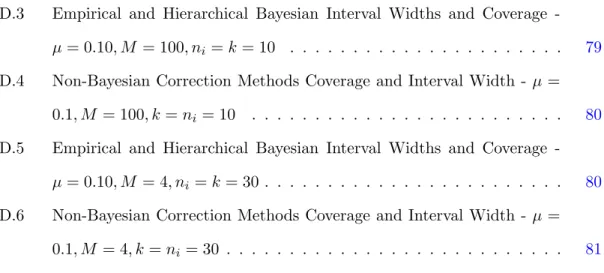
Of interest are the cases where the empirical Bayesian interval width is larger than the full hierarchical Bayesian interval width. Consider the distribution of the ratio of the empirical Bayesian interval widths using the method of moments estimator to full hierarchical Bayesian interval width using Haldane’s prior, seen below in Figure 3.1.
Figure 2.2 Ratio of Empirical Bayesian Interval Widths by Method of Moments to Hierarchical Bayesian Interval Widths by Haldane’s Prior
In the simulated data set, 23.35% of empirical Bayesian intervals using the method of mo-ments estimator are longer than the hierarchical Bayesian intervals. Conversely, the empirical Bayesian interval width using the maximum likelihood estimator is larger than the full hierar-chical interval width in all but approximately 1% of cases for all three Bayesian priors. This may be attributed to simulation error from the MCMC procedure — that is, if the empirical
Bayesian and analytical Bayesian interval widths are very, very close, then there is a probability that the MCMC approximation to the Bayesian interval width will be larger than the empiri-cal Bayesian interval width due simply to natural variation in the samples from the posterior distribution.
2.3.7 Analysis of Phenomenon
An interesting question exists as to when empirical Bayesian methods may, depending on the choice of estimation method and prior distribution, produce an interval that is longer than an interval produced by a full hierarchical Bayesian analysis (this will henceforth be referred to simply as “the phenomenon”). It should be stated beforehand that since the Bayesian analysis is driven by the likelihood, an empirical Bayesian analysis using a maximum likelihood estimator generally can not be larger than a full hierarchical Bayesian analysis except in an informative prior setting. For other estimators, the chances are dependent on the shape of the posterior distribution.
Suppose that yi successes are observed in ni trials for some observation i, still with known
variance parameterM. In the traditionalα, βform, the parameters of empirical Bayes posterior distribution are given as
˜
αi =yi+ ˆµM
˜
βi =ni−yi+ (1−µˆ)M
These may be converted back to to µ, M notation as
˜ µi= yi+ ˆµM yi+ ˆµM +ni−yi+ (1−µˆ)M = yi+ ˆµM ni+M (2.16) ˜ Mi =yi+ ˆµM+ni−yi+ (1−µˆ)M =ni+M (2.17)
Taking the expected value, the empirical Bayesian estimator is ˆθi = ˜µi. The empirical
Bayesian interval, however, depends on more than just the estimator - an important feature is the shape of the two posterior distributions. Unlike the normal, the beta distribution is
flexible in shape and bounded on either side - for example, if one of α orβ (in the traditional parametrization) is larger than 1 and the other smaller than 1, then as Casella and Berger (2002) notes the resulting distribution will be J-shaped, not unimodal. Even if the distribution is unimodal, it need not be symmetric, as seen in Figure 2.1.
The form of the empirical Bayesian posteriors is a beta distribution. Empirical evidence suggests that the full Bayesian posterior using Haldane’s prior (equation (2.14)) is very well approximated by a beta distribution with mean and variance
E[θi] = ˜µ= ˜µi= yi+ ˆµM LEM ni+M (2.18) V ar(θi) = ˆ µM LE(1−µˆM LE) (M+ni+ 1)c (2.19) and borrowing an approximation from Morris (1988), the constantcin equation (2.19) is given by
c= µ˜i(1−µ˜i)
˜
µi(1−µ˜i) +B2(ni+M)ˆµM LE(1−µˆM LE)/[k(niB+ (1−B)) + 1]
(2.20) whereB =M/(ni+M). This approximation works extremely well for the simulated data set
with M = 4 and k = ni = 10. For different values of M, k, and ni, simulations show the
approximation appears to hold well, even when ni is not constant for alli.
The approximation is further explored and justified in Chapter 3; however, a “conjugate-type relation” in the hierarchical beta-binomial model was noticed by Lee and Sabavala (1987) for a beta prior on the mean (and note that Haldane’s prior is a beta distribution with pa-rameters α =β = 0), and Morris (1988) pretends the marginal distribution of the yi given µ
and M is a member of the natural exponential family in order to derive an exact conjugacy for the approximate distribution. In simulations, the relationship appears to be close to exact. Empirically, the root mean squared difference (over all θi estimates in all data sets) between
the MLE and hierarchial Bayesian estimators for each of the θi is 0.000285, as compared to
a 0.005944 (over 20 times larger) root mean squared difference between the MM and hierar-chical Bayesian estimators for the θi. The idea of matching posterior estimates to frequentist
mode rather than the posterior mean. A brief discussion of the history of matching posterior moments to frequentist estimates is provided in Ghosh and Liu (2011), along with examples of priors that, up to a high order of approximation, have posterior expectation matching the maximum likelihood estimate in the univariate and multivariate (but not hierarchical) case.
Unlike the normal density, the variance of the beta distribution is a function of the mean µ — for a fixedM, the variance is maximized atµ= 0.5 and decreases as µmoves towards 0 or 1, and the distribution will become more compact. As this occurs, central intervals taken from that distribution will necessarily have a smaller width. Furthermore, the distribution is flexible and shape and the skew increases as the mean moves away from µ= 0.5.
The phenomenon occurs when the empirical Bayesian posterior distribution based on an estimator ˆµ gains enough additional interval width from the increased posterior variance of ˆµ being larger than ˆµM LE and from the shape of the posterior becoming more symmetric as ˆµ
moves away from the boundary of the parameter space towards 0.5 to overcome the additional variance gained from the full hierarchical model (for Haldane’s prior the proportion increase is given by 1c from equation (2.20), though the changing shape of the posteriors means that the required increase in ˆµ is different than the simple ratio of variances). The result is that there exists a value r such that if ˆµ/µˆM LE > r, then the empirical Bayesian interval width will be
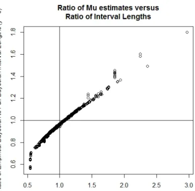
larger than the full hierarchical Bayesian width. This can be seen in the pattern of Figure 2.3
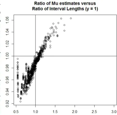
Figure 2.3 Ratio of Empirical Bayesian Interval Width using Method of Moments over Aver-age (Within Data Set) Hierarchical Bayesian Interval width using Haldane’s Prior versus Ratio of ˆµ Estimates (Method of Moments Over Maximum Likelihood) for yi = 0
The phenomenon occurs when ˆµM M is about r = 7.4% larger than ˆµM LE, though the exact
value of r may vary slightly depending on the specific estimates. It can also be seen when yi 6= 0. Supposingyi= 1 shows a similar pattern in Figure 2.4below.
Figure 2.4 Ratio of Empirical Bayesian Interval Width using Method of Moments over Aver-age (Within Data Set) Hierarchical Bayesian Interval width using Haldane’s Prior versus Ratio of ˆµ Estimates (Method of Moments Over Maximum Likelihood) for yi = 1
The phenomenon occurs when ˆµM M is about r= 8.8% larger than ˆµM LE.
Similar results may be shown for any arbitraryyi, though asyi/nimoves further away from
0 or 1, the effect (and the underestimation of the variance) decreases as posterior mean move closer to 0.5. Furthermore, though these simulations have assumed ˆµM LE <0.5, results will
apply with inverted equalities when ˆµM LE >0.5.
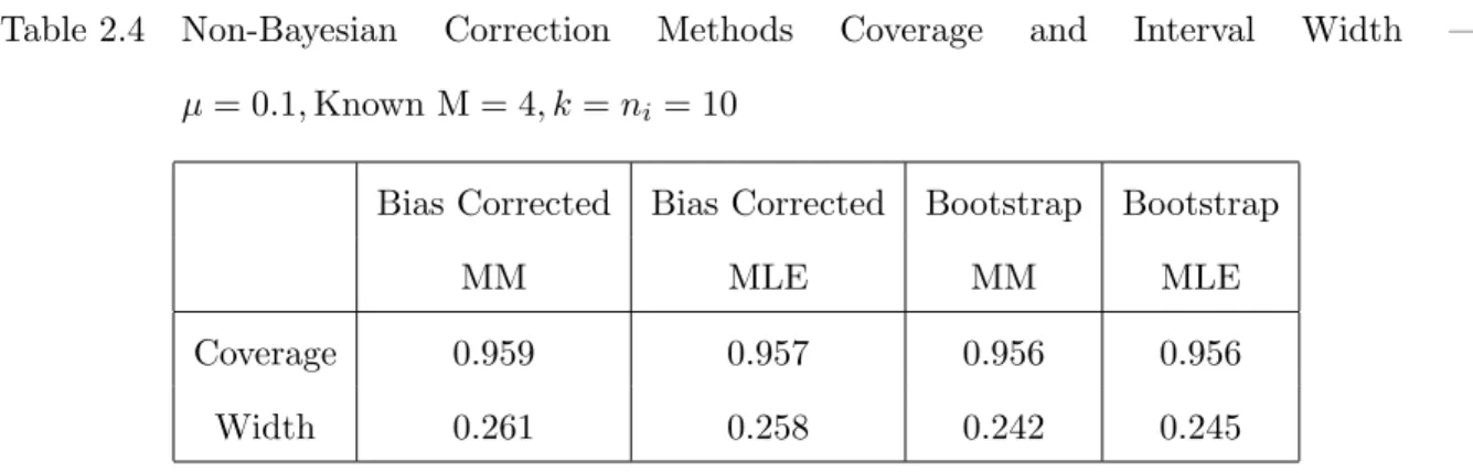
2.3.8 Non-Bayesian Methods
It is useful to compare the coverage and average interval width for the simulated data of Section 2.3.6 to the non-Bayesian methods described in Section 2.1. The bias correction and parametric bootstrap methods were considered for both the method of moments (MM) and
maximum likelihood estimators (MLE). Unconditional coverage and average interval width are given by
Table 2.4 Non-Bayesian Correction Methods Coverage and Interval Width — µ= 0.1,Known M = 4, k=ni = 10
Bias Corrected Bias Corrected Bootstrap Bootstrap
MM MLE MM MLE
Coverage 0.959 0.957 0.956 0.956
Width 0.261 0.258 0.242 0.245
Despite bias correction method being intended to “correct” the interval width as opposed to simply widen it, the bias correction method actually performs the worst — the coverage is slightly above 95%, but at the cost of the interval width being, on average, even longer than the full Bayesian solution. The bootstrap method performs similarly to the full Bayesian analysis shown in Table3.1, which is no surprise given that the bootstrap approximates a full Bayesian solution.
Further simulation studies were conducted in order to determine under what conditions the phenomenon is likely to occur and, in general, to compare interval width correction methods based on the beta-binomial model, with the result being that the phenomenon is most likely to appear when ˆµis near 0 or 1 and M is small, corresponding to data sets with lots of group proportions near 0 or 1, as in the terbinafine data given in Appendix B. These results are described in AppendixC.
2.3.9 Unknown M
In most situations, the variance parameter M (or, equivalently, the dispersion parameter φ) must also be estimated. It is easiest to use the parametrization in equation (2.8) in order to specify priors onφ. Since bothµandφare bounded by 0 and 1, beta distributions are obvious choices. In fitting with the previously discussed framework, priors that match the moments of the hyperpriors to the empirical Bayesian estimates are used.
µ∼Beta(ˆµ,2) φ∼Beta( ˆφ,2)
(2.21)
In this way, each prior has expectation equal to the empirical Bayesian estimates, but suffi-ciently diffused. This may be used as an alternative to the Morris-style method of comparison, as the empirical Bayesian estimates using each method can be constructed as the result of a full hierarchical Bayesian analysis with the above priors placed on each parameter, but with the hyperprior variance parameterM0(equal to 2 in the cases above) going to infinity to create
degenerate distributions that take the empirical Bayesian prior estimate with probability 1. The above prior will yield a proper posterior so long as ˆµ and ˆφ are not either zero or one, corresponding to extreme scenarios under which the beta-binomial model would not typically be considered.
In order to approximate the Morris-style comparisons, the following priors will be used
µ∝ 1
µ(1−µ) φ∼Beta(0.5,1)
(2.22)
The posterior expectation of the full beta-binomial model will very loosely approximate the empirical Bayesian estimate using the method of maximum likelihood, though the approx-imation is not nearly as close to exact as the Haldane’s prior for the known M case. It will become very close as the sample sizesni and kincrease, as shown in the results of the
Terab-ifine analysis in Table 2.1. Simply taking µ∼Beta(0,0) and φ∼Beta(0,0) as in the case of known M generally does not approximate posterior means well for smallerM values, possibly due to unaccounted for covariance between ˆµ and ˆM when ˆM is small. Efforts to determine a weakly informative or or noninformative set of priors that produced posterior estimates of θi strongly approximating empirical Bayesian estimates using any estimator were unsuccessful,
and it is unclear whether such priors exist. The set of priors in (2.22) produces Morris-style approximations for many different (but not all) data sets. As the prior on φ is proper, the posterior distribution is guaranteed to be proper so long asyi 6= 0 for alliandyi 6=ni for alli.
2.3.10 Further Simulations
A simulation study was performed, simulating data from a beta-binomial distribution with µ= 10, M = 4, and k= 10 binomial observations of ni = 10 trials each. Intervals compared
were the method of moments and method of maximum likelihood empirical Bayesian methods and full Bayesian hierarchical analyses using the priors described in equations (2.21) (matching both methods of empirical Bayesian estimation) and the priors described in equations (2.22). Coverage and average interval widths are shown below in Table2.5.
Table 2.5 Empirical and Hierarchical Bayesian Interval Widths and Coverage -µ= 0.10, M = 4, ni =k= 10
EB MM EB MLE Intermediate Prior Intermediate Prior Approx. Morris
Matching Matching Matching
ˆ
µM M,φˆM M µˆM LE,φˆM LE Prior
Coverage 0.842 0.838 0.894 0.894 0.941
Width 0.221 0.220 0.229 0.229 0.245
The underlying problem with the use of empirical Bayesian analysis is much more apparent — using either estimation method, the empirical Bayesian intervals do not achieve nominal 95% coverage. Matching empirical Bayesian estimates to hierarchical prior means does not necessarily provide nominal coverage in this scenario; however, the noninformative prior that approximates Morris-style matching performs better, achieving almost nominal coverage.
The set of priors used in equation (2.22) does not match the empirical Bayesian results nearly as well as in the case with known M. The root mean squared difference between the MLE empirical Bayesian estimates for θi and approximate Morris matching Bayesian hierarchical
estimates was 0.0467, as compared to 0.0471 using the MM empirical Bayesian estimates. Though they produced undercoverage, the intermediate priors of equation (2.21), however, had a root mean squared difference of 0.0231 for the MLE empirical Bayesian estimator and 0.0240 for the MM empirical Bayesian estimator.
Table 2.6 Non-Bayesian Correction Methods Coverage and Interval Width — µ= 0.1, M = 4, k=ni= 10
Bootstrap Bootstrap Bias Correction Bias Correction
MM MLE MM MLE
Coverage 0.939 0.917 0.944 1
Width 0.245 0.241 0.461 0.89
Non-Bayesian methods in this scenario provided mixed results. The bootstrap approach performs decently, with average coverage and width similar to the full hierarchical Bayesian analysis in the method of moments case, though there tends to be undercorrection in the case of the maximum likelihood estimator. The bias correction approach breaks down, though this is partly due to occasional poor estimates of the variance parameter M in the bootstrap procedure.
Further simulations were again conducted in order to determine the appearance of the phenomenon and to determine appropriate priors for comparison to the empirical Bayesian intervals — in general, the bias correction technique fails when the posterior distribution is not sufficiently normal, while the bootstrap performs well. For a large M value, the intermediate priors of equation (2.21) show near nominal coverage. These results are described in Appendix
D.
2.3.11 Recommendations
For the case of known variance parameter M, the empirical Bayesian interval may be compared to a Bayesian interval produced by using a diffuse prior with mean ˆµ— the particular choice of estimator does not appear to matter. By fully diffusing to Haldane’s prior, however, empirical Bayesian interval widths produced from the method of maximum likelihood can be directly compared in the Morris style. Even without using Haldane’s prior, however, a general noninformative prior on µ should produce excellent results. For the method of moments, the Bayesian width using Haldane’s prior may still be useful for comparison if one is not concerned
about matching posterior expectations, and may indicate intervals that are inappropriately centered and, hence, too long. If one is concerned about matching posterior expectations, the bootstrap correction method appears to offer the best coverage.
For the case of unknown variance parameter M, the situation is not as clear, as there is no known prior that necessarily matches posterior Bayesian estimates to empirical Bayesian estimates for any method of estimation. Depending on the data set, using Haldane’s prior on µ and a Beta(0.5,1) prior on φ or beta priors that match means of µ and θ to empirical Bayesian estimates may tend to provide nominal coverage, and can be used for comparison. In all cases, the parametric bootstrap of Laird and Louis (1987) will produce useful intervals that match the posterior expectation, though coverage may be slightly more or less than the nominal amount, and interval widths may be longer than a corresponding Bayesian solution that produces nominal coverage.
2.4 Future Work
Further work on this project is possible. Several theoretical results have been stated with little justification, though the works of Carl Morris (particularly Morris (1988)) provide some evidence for the approximations used in this paper, and are further explored in Chapter3. Prior selection for the case of unknown variance parameter M remains undeveloped. Simulations suggest that simply taking diffuse beta priors on µ and φ with expectation equal to ˆµ and ˆφ does not produce nominal coverage for small M values, corresponding to a large spread of θi
values, though as the data-generatingM increases and the spread ofθi decreases (approaching
a simple binomial model with fixed probability of success θ) these intermediate priors perform increasingly well.
2.5 Conclusion
In general, the idea of underestimation of the variance is well-defined in the normal-normal case. Stepping outside of that particular model, however, ideas do not apply as neatly, as for a given set of empirical Bayesian estimates ˆθi, there may not exist a hierarchical Bayesian prior
which produces posterior estimates for the θi equivalent to the empirical Bayesian estimates.
Even if there exists a prior which offers a close approximation, the existence of multiple es-timation techniques makes it entirely possible to have an empirical Bayesian interval based upon some consistent estimator which produces an interval width larger than the hierarchical Bayesian interval. The types of data sets where these phenomenon may occur — small sample data sets, with observations tending near zero or one — are often the types where Bayesian and empirical Bayesian techniques are the most useful, and the difference in interval width may be non-trivial.
Non-Bayesian correction methods have issues as well. The bias correction method intended to “correct,” rather than simply widen, appears to perform poorly in the small sample beta-binomial case, and while the parametric bootstrap correction method is superior at producing interval estimates which achieve nominal unconditional coverage, in its basic form it is arti-ficially creating a prior around an estimate rather than matching a known hierarchical prior. There is no clear reason why this should be considered ”correct,” especially if there exists a hierarchical prior that produces near-nominal coverage and a shorter interval width.
An alternative method of comparison is given by an intermediate vague prior with mean given by estimates of prior parameters. This method focuses less on the idea of correcting empirical Bayesian intervals by matching empirical Bayesian estimates exactly to expectations of hierarchical Bayesian models, but does provide a framework under which the hierarchical prior used in Morris-style corrections for the normal-normal model can be shown as a limit of the intermediate prior density, and a similarly limiting density under the beta-binomial model matches and can be used to quantify the underestimation in variance in when using the maximum likelihood estimator and provide an appropriate width correction with other estimators. In the case of known shrinkage parameter B, this provides excellent nominal coverage. In the case of unknown shrinkage parameter, the method generally produces good (though not necessarily nominal) coverage in many cases and often outperforms non-Bayesian correction methods, though further analysis is needed.
CHAPTER 3. COMPARISON FRAMEWORK FOR THE NATURAL EXPONENTIAL FAMILY WITH QUADRATIC VARIANCE
FUNCTIONS
3.1 NEFQVF Families
The results of Chapter 2 may be extended to a larger class of models, of which the beta-binomial is a member - the natural exponential family with quadratic variance function (NE-FQVF). In this chapter, properties of the NEFQFV family will be identified as relating to empirical Bayesian analysis, and some approximations for posterior distributions will be given and discussed, along with a framework for comparisons of widths of empirical Bayesian in-tervals, with a specific further application of the results to the gamma-Poisson model. These approximations can be used to refine a method from Morris (1988) for correcting empirical Bayesian interval widths with known shrinkage amount, and simulations for this method using the beta-binomial and gamma-Poisson models show near-nominal coverage.
3.1.1 NEFQVF Distributions
Properties of NEF and NEFQVF distributions have been studied and enumerated in Morris (1982), Morris (1983a), and Morris and Lock (2009), which define and give basic properties of NEFQVF distributions, combine and present statistical theory for NEFQVF distributions, and show connections among NEF and NEFQVF distributions, respectively. Sections3.1.1and
3.1.2will draw and intermix results from these papers freely. Members of the NEFQVF family are, as the name implies, members of the natural exponential family, and hence have densities that may be written proportional to