An Alternative Approach to Estimation of Population Mean in Two-Stage Sampling

(1)

72

An Alternative Approach to Estimation of Population

Mean in Two-Stage Sampling

Ravendra Singh1*, P.C. Gupta1, Sarla Pareek1, Gajendra K. Vishwakarma2

1.Department of Mathematics & Statistics,Banasthali University, Jaipur- 304022, Rajasthan, India [email protected]

2.Department of Applied Mathematics, Indian School of Mines, Dhanbad - 826004, Jharkhand, India [email protected]

Abstract

This paper considers the problem of estimating the population mean in two-stage sampling with unequal first stage unit (fsu) for ratio, product and regression estimators when the population mean of the auxiliary variable is not known in advance. The ratio, product and regression estimators are suggested and studied their properties. It is shown that under certain conditions the suggested estimators are more efficient than than Sukhatme et al (1984) estimators. Numerical illustration is given in support of present study.

Keywords: Auxiliary variate, study variate, mean squared error, two-stage sampling, ratio estimator, product estimator, regression estimator.

Mathematics Subject Classification: 62D05. 1. Introduction

In survey sampling, the use of auxiliary information can increase the precision of an estimator when study variable y is highly correlated with the auxiliary variable x. but in several practical situations, instead of existence of auxiliary variables there exists some auxiliary attributes, which are highly correlated with study variable y, such as (i) Amount of milk produced and a particular breed of cow. (ii) Yield of wheat crop and a particular variety of wheat etc. In such situations, taking the advantage of point bi-serial correlation between the study variable and the auxiliary attribute, the estimators of parameters of interest can be constructed by using prior knowledge of the parameters of auxiliary attribute.

The problem of the estimation of population parameters like mean, variance, and ratio of two population means are common in agriculture, economics, medicine, and population studies. The use of auxiliary information has been applied for improving the efficiencies of the estimators of population parameter(s) irrespective of sampling design. Ratio, product and regression methods of estimation are good examples in this context. Cochran (1940) used auxiliary information at the estimation stage and proposed a ratio estimator for the population mean. A ratio estimator is preferred when the correlation coefficient between the study variate and the auxiliary variate is positive. Robson (1957) defined a product estimator that was revisited by Murthy (1964). The product estimator is used when the correlation between the study variate and the auxiliary is negative.

The use of auxiliary information has to a fairly large extent proved to be effective approach in increasing the precision of estimates in survey sampling. Many estimators of the finite population parameter have been constructed using auxiliary information. Information on variables correlated with the main variable under study is popularly known as auxiliary information which may be fruitfully utilized either at planning stage or design stage or at the estimation stage to arrive at an improved estimate compared to those not utilizing it. The use of auxiliary information dates back to 1820 with a comprehensive theory provided by Cochran (1977). Recently, several authors like Samiuddin and Hanif (2007), Kadilar and Cingi (2004, 2005), Pradhan (2005), Sahoo and Panda (1997, 1999) and Upadhyaya and Singh (1999) have worked on the use off auxiliary information in survey sampling.

In some cases information on auxiliary variables may be readily available on all units in the population; however, this is not always the case in certain practical situations. Hence, we rely on taking a fairly large sample from the

N

unit in the population in order to estimate the population mean of the auxiliary variable(s).

Since it is assumed that the population mean

X

, of the auxiliary variable, is unknown, we first select a preliminary large sample of size

n′

from

N

units in the population by simple random sampling without replacement in order to provide an estimate of

X

. Let

U

be a finite population partitioned into

n′

First Stage Units (FSU) denoted by

U

₁

,

U

₂

,...,

U

_I

,...

U

_n_′ such that the number of Second Stage Units (SSU) in

U

_i is

i

M

. Let

y

and

x

be the variable under study and auxiliary variable taking the values

y

_ij and

x

_ij

respectively, for the

j

th_{SSU on the unit}

U

_i

(

i

=

1

,

2

,...,

n

′

;

j

=

1

,

2

,...,

M

_i

)

.

∑

=

Mi j ij i i

P

M

P

1

;

∑

′ =

′

=

n i i

P

n

P

1

;

P

=

X

,

Y

.

(2)

73

Assume that a sample

s

of

n

FSU’s is drawn from

U

and then a sample

s

_i of

m

_i SSU’s from the

i

th

selected FSU from

U

_i using simple random sampling without replacement.

∑

=

i m j ij i i

p

m

p

1

;

∑

=

n i i

p

n

p

1

;

p

=

x

,

y

.

When

X

is known, the classical two-stage ratio, product and regression estimators of

Y

with unequal FSU and their corresponding approximate Mean Square Error (MSE) has been given by Sukhatme et al (1984) and are as presented below: Ratio estimator:

x

X

y

1

=

(1) 2 2 1 2 2 1 1 Ri N i i R

S

)

y

(

MSE

∑

=

+

=

λ

Product estimator

X

x

y

2

=

(2)

( )

∑

=

+

=

N i Pi i P

S

y

MSE

1 2 2 2 2 1 2

λ

Regression estimator

y

₃

=

y

+

β

(

X

−

x

)

(3)

( )

∑

=

+

=

N i Bi i B

S

y

MSE

1 2 2 2 2 1 2

λ

where

n

f

−

=

1

λ

;

N

n

f

=

;

(

)

i i i i

nNm

f

M

2 ₂ 2

1

−

=

λ

; i i i

M

m

f

2

=

; xy x y R

S

R

S

RS

S

1 2 1 2 2 1 2 1

=

+

−

2

;

S

P

S

y

R

S

x

RS

1xy 2 1 2 2 1 2 1

=

+

2

;

S

B

S

y

B

S

x

BS

1xy 2 1 2 2 1 2 1

=

+

−

2

; xyi xi yi Ri

S

R

S

RS

S

₂2

=

₂2

+

2 ₂2

−

2

₂ ;

S

₂2_Pi

=

S

₂2_yi

+

R

2

S

₂2_xi

+

2

RS

₂_xyi; xyi xi yi Bi

S

B

S

BS

S

₂2

=

₂2

+

2 ₂2

−

2

₂ ;

∑

(

)

′ =

−

′

=

n i i p

P

n

S

1 2 2 1

1

;

∑

(

)

′ =

−

′

=

n i i ij Pi

P

n

S

1 2 2 2

1

;

(

)(

)

∑

′ =

−

′

=

n i i i PQ

P

Q

n

S

1 1

1

;

(

)(

)

∑

′ =

−

′

=

n i i ij i ij PQi

P

Q

n

S

1 2

1

;

P

=

x

,

y

;

Q

=

x

,

y

and

P

≠

Q

. 2 1P

S

and

S

22Pi are the variance among FSU means and variance among subunits for the th

i

FSU while

S

1PQ

and

S

₂_PQi are their corresponding co-variances.

Sahoo and Panda (1997, 1999) described class of estimators in two stage sampling with varying probabilities and later examined family of estimators using auxiliary information in two-stage sampling. Scott and Smith (1967) and Chaudhuri and Stenger (1992) described the prediction criterion for two-stage sampling while Hossain and Ahmed (2001) examined the class of predictive estimators in two-stage sampling using auxiliary information. 2. Suggested Estimators

RATIO ESTIMATOR

Under the assumptions above, the estimator

y

₁ will take the form

x

y

=

′

* * * 1 (4)

(3)

74 If we express (4) in terms of

d

’s 2 1 1 * 1

(

1

)(

1

)(

1

)

−

+

=

Y

d

y

o (5)

Expanding the right hand side of (5) neglecting terms involving power of this greater than two, we have

(

)

2 1 2 1 1 0 2 0 2 1 0 1

Y

1

d

y

∗

=

+

−

+

−

+

y

₁*

−

Y

=

Y

(

d

₀

−

d

₁

+

d

₂

+

d

₀

d

₂

−

d

₀

d

₁

−

d

₁

d

₂

+

d

₁2

)

(6) Squaring both sides of (6) and neglecting terms involving powers greater than two, we have

(

y

₁∗

−

Y

)

2

=

Y

2

(

d

₀2

+

d

₁2

+

d

₂2

+

2

d

₀

d

₂

−

2

d

₀

d

₁

−

2

d

₁

d

₂

)

(7) By taking expectations of both sides by (7) and simplifying we get the MSE of as

( )

∑

′ = ′ ′ = ∗

=

′

+

−

n i Ri i R n i Ri i R

S

y

MSE

1 2 2 3 2 1 3 1 2 2 2 2 1 1

λ

(8) where

S

R

S

x

RS

1xy 2 1 2 2 1 ′

=

−

2

;

S

Ri

R

S

xi

RS

2xyi 2 2 2 2 2 ′

=

−

2

PRODUCT ESTIMATOR is defined as

x

y

′

=

∗ ∗ 2

Following the procedure of section 2 it is easy to verify that the MSE of

y

∗₂ is

( )

∑

′ = ′ ′ = ∗

=

′

+

−

n i Pi i P n i Pi i P

S

y

MSE

1 2 2 3 2 1 3 1 2 2 2 2 1 2

λ

(9) where,

S

_P

R

S

2_x

RS

₁_xy 1 2 2 1 ′

=

+

2

;

S

Pi

R

S

xi

RS

2xyi 2 2 2 2 2 ′

=

+

2

REGRESSION ESTIMATOR is defined by

y

3*

=

y

*

+

β

ˆ

*

(

x

'

−

x

*

)

where _*₂ * *

ˆ

x xy

s

=

β

is an estimator of 2 x xy

S

=

β

. It is easy to verify that

s

*_xy and

s

*_x2are unbiased for

S

_xyand

2 x

S

respectively. Let

y

=

Y

(

1

+

d

0

)

∗ ,

x

∗

=

X

(

1

+

d

₁

)

,

x

′

=

X

(

1

+

d

₂

)

such that

E

( )

d

_P∗

=

0

;

( ) ( )

₂ 2 ∗ ∗

=

∗

P

V

d

E

_P ;

(

)

(

_∗ _∗

)

∗ ∗

=

∗ ∗

Q

P

Q

P

Cov

d

E

_P

,

_Q

,

;

( )

₂2

( )

₂

X

x

V

d

E

=

′

;

(

)

(

)

X

P

x

P

Cov

d

E

_P _∗ ∗

′

=

∗

,

2

Under TSS with unequal FSU

( )

∑

′ = ∗ ∗ ∗

+

′

=

n i i P i P

S

P

V

1 2 2 2 2 1

λ

;

(

)

∑

′ = ∗ ∗ ∗ ∗ ∗ ∗

+

′

=

n i i Q P i Q P

S

Q

P

Cov

1 2 2 1

,

λ

;

n

f

₁

1

−

=

′

λ

;

n

f

′

=

1 ;

( )

2 2 1 3 2 1 3 xi N i i x

S

x

V

∑

=

+

=

′

λ

;

(

)

∑

= ∗

′

=

+

N i xyi i xy

S

x

P

Cov

1 2 2 3 1 3

,

λ

; where

n

f

′

−

=

1

3

λ

;

N

n

f

′

=

′

;

(

)

i i i i

Nm

n

f

M

′

−

=

2 2 3

1

λ

;

P

∗

=

x

∗,

y

∗,

x′

;

Q

∗

=

x

∗,

y

∗ and ∗ ∗

≠

Q

P

.

The large sample approximation to the MSE of

y

₃* is given by

( ) ( )

∗

=

∗

+

(

′

−

∗

)

+

(

∗

′

−

∗

)

x

,

y

BCov

x

V

B

y

V

y

MSE

₃ 2

2

(4)

75

If the values of the variance and covariance terms defined in section 2 are correspondingly substituted into (11), the MSE of

y

₃* after simplification becomes

( )

∑

′ = ′ ′ ′ = ∗

=

′

+

−

n i i B i B n i Bi i B

S

y

MSE

1 2 2 3 2 1 3 1 2 2 2 2 1 3

λ

(12) where

S

₁2_B

=

B

2

S

₁2_x

−

2

BS

₁_xy

,

S

₂2_Bi

=

B

2

S

₂2_xi

−

2

BS

₂_xyi

Remark 1: it will be observed that the MSEs of the estimators

y

₁∗

,

y

₂∗ and

y

₃* each consist of four components. The first two components on the right hand sides of (8), (9) and (12) represents the additional contribution to the variance arising due to the fact that the values determined from the large sample of size n’ are subject to error while the last two components represent the variance of the estimates if n’ where equal to N. The estimators under consideration require the advance knowledge of some population parameters which are usually unknown. However in practice, the results from previous experience (survey) or the sample estimators of their population parameters may be substituted for this purpose. Although, the estimation may turn out to be biased the bias would be negligible in large samples and the approximate MSEs to order one will be the equivalent to those derived and for large samples, the difference would be minimal.

3. Efficiency Comparison

In this section, we considered the theoretical comparison of the performances of the suggested estimators with respect to Sukhatme et al (1984) estimators. It is easily seen that when we subtract (1), (2) and (3) from (8), (9) and (12) respectively we get:

Ratio estimation: 2 2 1 3 2 1 3 1 Ri n i i R

S

∑

=

+

≤

λ

Product estimation: 2 2 1 3 2 1 3 1 pi n i i P

S

∑

=

+

≤

λ

Regression estimation: 2 2 1 3 2 1 3 1 Bi n i i B

S

∑

=

+

≤

λ

where ₁ 1

S

₁2_R

n













−

=

θ

λ

; ₂ 1

S

₁2_B

n













−

=

θ

λ

Thus, we see that the estimators

y

₁∗

,

y

₂∗ and

y

3* will be more efficient than

y

1

,

y

2 and

y

3 respectively, since 1

λ

and

λ

₂ will always be negative.

4. Numerical Illustration

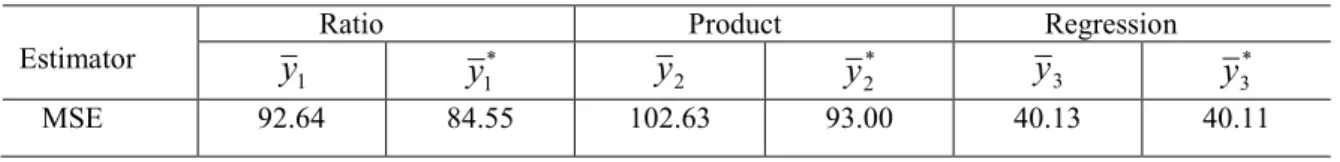
The preceding theoretical results shall now be illustrated with reference to the data given by Okafor (2002) pp 223-224. Taking N=92, n’=26 and replacing the population values of (1), (2), (3), (8), (9) and (12) by their estimate obtained from the sample, the MSE for the different estimators are presented in table 1.

Table 1: MSE for the different estimators

Estimator

Ratio Product Regression

1

y

* 1

y

2 * 2

y

3 * 3

y

MSE 92.64 84.55 102.63 93.00 40.13 40.11 5. Conclusion

Table 1 clearly indicates that

MSE

(

y

₁*

)

is smaller than

MSE

(

y

₁

)

,

MSE

(

y

₂*

)

is smaller than

MSE

(

y

₂

)

. Hence,

y

₁* and

y

₂* is certainly to be preferred in practice. Also we see that the

MSE

(

y

3*

)

is smaller than

(5)

76

)

(

y

₃

MSE

although the difference is not appreciable. This is an expected result since the conditions given in section 3 is satisfied. Note that

R

ˆ

=

1

.

21

is substantially different from

β

ˆ

=

0

.

1

the regression coefficient, this means that the regression line does not pass through the origin; and this goes further to explain why the regression estimators are better than the ratio and product estimators. It is therefore concluded that, for this data set the suggested estimators are more efficient than Sukhatme et al (1984) estimators.

References

Chaudhuri, A. and Stenger, H. (1992): Survey sampling theory and methods. Mracel Decker, Inc. New York. Cochran W.G. (1940): The estimation of the yields of the cereal experiments by sampling for the ratio of gain to total produce. Journal of Agricultural Science, 30, 262-275.

Cochran, W.G. (1977): Sampling techniques. 3rd edition. John Wiley, New York.

Hossain, M.I., and Ahmed, M. S. (2001): A class of predictive estimators in two-stage sampling using auxiliary information. Information and Management Sciences, 12, 1, 49-55.

Kadilar, C. and Cingi, H. (2004): Estimator of a population mean using two auxiliary variables in simple random sampling, International Mathematical Journal, 5, 357–367.

Kadilar, C. and Cingi, H. (2005): A new estimator using two auxiliary variables, Applied Mathematics and Computation, 162, 901–908.

Murthy, M.N. (1964): Product method of estimation, Sankhya, A, 26, 69-74.

Okafor, C.F. (2002): Sample survey theory with applications. Afro-Orbis Publications Ltd Nsukka.

Pradhan, B.K. (2005): A chain regression estimator in TPS using multi-auxiliary information. Bulletin Malaysian Mathematical Sciences, 28, 1, 81-86.

Robson, D.S. (1957): Application of multivariate polykays to the theory of unbiased ratio-type estimation.

Journal of American Statistical Association, 52, 511-522.

Sahoo, L.N. and Panda, P. (1997): A class of estimators in two-stage samplings with varying probabilities. South African Statistical Journal, 31, 151–160.

Sahoo, L.N. and Panda, P. (1999): A class of estimators using auxiliary information in two-stage sampling.

Australian and New Zealand Journal of Statistics, 41, 4, 405–410.

Samiuddin, M. and Hanif, M. (2007): Estimation of population mean in single phase and two phase sampling with or with out additional information. Pakistan Journal of Statistics, 23, 2, 99-118.

Scott, A. and Smith, T.M.P. (1969): Estimation in multistage sampling. Journal of American Statistical Association, 64, 830-840.

Sukhatme, P.V., Sukhatme, B.V., Sukhatme, S. and Ashok, C. (1984): Sampling theory of surveys with applications. Iowa State University Press, USA.

Upadhyaya, L. N., and Singh, H. P. (1999): Use of transformed auxiliary variable in estimating the finite population mean. Biometrical Journal, 41, 627-636.