Accelerating Large-scale Multi-objective Optimization via Problem Reformulation

(1)

Accelerating Large-Scale Multi-Objective

Optimization via Decision Space Reconstruction

Cheng He, Lianghao Li, Ye Tian, Xingyi Zhang

IEEE Member, Ran Cheng

IEEE Member,

Yaochu Jin

IEEE Fellow

and Xin Yao

IEEE Fellow

Abstract—In this work, we propose a framework to accelerate the computational efficiency of evolutionary algorithms on large-scale multi-objective optimization. The main idea is to track the Pareto optimal set directly via decision space reconstruction. To begin with, the algorithm obtains a set of reference directions in the decision space and associates them with a set of weight variables for locating the Pareto optimal set. Afterwards, the decision space is reconstructed by taking the weight variables and their corresponding solutions as the input and output of the reconstructed optimization problem, respectively. Thanks to the low dimensionality of the weight variables, a set of quasi-optimal solutions can be obtained efficiently. Finally, a multi-objective evolutionary algorithm is used to spread the quasi-optimal solutions over the approximate Pareto optimal front uniformly. Experiments have been conducted on a variety of large-scale problems with 2 or 3 objectives and up to 1000 decision variables. Four different types of well-known algorithms are embedded into the proposed framework and compared with their original versions, respectively. Furthermore, the proposed framework has been compared with two state-of-the-art algorithms for large-scale multi-objective optimization. Experimental results have demonstrated the significant improvement benefited from the framework in terms of its performance and computational efficiency in large-scale multi-objective optimization.

Index Terms—Large-scale optimization, multi-objective opti-mization, evolutionary algorithms, decision space reconstruction

I. INTRODUCTION

Many real-world optimization problems involve multiple conflicting objectives [1], [2], known as multi-objective op-timization problems (MOPs), which can be mathematically formulated as follows:

Minimize F(x) = (f1(x), f2(x), . . . , fM(x)) (1)

subject to x∈X,

C. He, R. Cheng, and X. Yao are with the Department of Computer Science and Engineering, South University of Science and Technology, Shenzhen 518055, China. X. Yao is also with Center of Excellence for Research in Computational Intelligence and Applications (CERCIA), School of Computer Science, University of Birmingham, Birmingham B15 2TT, United Kingdom. E-mail: [email protected], [email protected], [email protected]. (Corresponding author: Ran Cheng)

L. Li is with the Key Laboratory of Image Information Processing and Intelligent Control of Education Ministry of China, School of Automation, Huazhong University of Science and Technology, Wuhan 430074, China. E-mail: [email protected].

Y. Tian and X. Zhang is with the Key Lab of Intelligent Comput-ing and Signal ProcessComput-ing of Ministry of Education, School of Computer Science and Technology, Anhui University, Hefei 230039, China. E-mail: [email protected].

Y. Jin is with the Department of Computer Science, Universi-ty of Surrey, Guildford, Surrey, GU2 7XH, United Kingdom. Email: [email protected].

where X is the search space of decision variables with

x=(x1, . . . , xD)denoting the decision vector [3]. Due to the

conflicting nature of the objectives, there does not typically exist a single solution that can minimize all the objectives simultaneously. Instead, a set of non-dominated solutions can be obtained as the trade-offs between different objectives [4], [5]. SupposexA,xBare two solutions of an MOP illustrated

by (1), solution xA is known to Pareto dominate solution xB (denoted as xA≺xB), if and only if fi(xA)≤fi(xB)

(∀i∈{1,2, . . . , M}) and there exists at least one objective fj (j∈{1,2, . . . , M}) satisfyingfj(xA)<fj(xB). The collection

of all the Pareto optimal solutions in the decision space is called the Pareto optimal set (PS), and the projection of PS in the objective space is called the Pareto optimal front (PF).

To solve MOPs, a variety of multi-objective evolutionary algorithms (MOEAs) have been proposed during the past two decades [6], including the Pareto-based MOEAs [7], [8], [9], the decomposition based MOEAs [10], [11], and the indicator-based MOEAs [12], [13], etc. Despite that most existing MOEAs have been well assessed on the MOPs with a small number of decision variables, their performance degenerates dramatically on MOPs with hundreds or even thousands of decision variables, i.e., the large-scale multi-objective opti-mization problems (LSMOPs) [14]. As the number of decision variables increases linearly, the volume (as well as complexity) of the search space will increase exponentially, and thus leading to the curse of dimensionality [15], [16]. Nevertheless, due to the high demands in efficient large-scale multi-objective optimization [17], [18], there has been a increasing interest in large-scale multi-objective optimization in recent years. Exist-ing approaches for large-scale multi-objective optimization can be roughly classified into three different categories as follows. The first category is known as the decision variable analysis based approaches. To be specific, in the MOEA based on de-cision variable analysis (MOEA/DVA), the dede-cision variables are divided into three types, i.e., position variables, distance variables and mixed variables. Then, the different types of decision variables are optimized using two different strategies, where the mixed variables are considered as distance variables in the optimization. Similarly, the decision variable clustering based large-scale MOEA (LMEA) [19] also divides the deci-sion variables into convergence-related and diversity-related variables using a clustering method, and the two types of decision variables are optimized using two different strategies by focusing on convergence and diversity respectively.

The second category applies the cooperative coevolution (CC) framework [20]. For example, the third-generation co-operative coevolutionary differential evolution algorithm

(2)

(C-CGDE3) [21] maintains several independent subpopulations, each of which is a subset of the equal-length decision variables obtained by variable grouping (e.g., random grouping [22], linear grouping [23], order grouping [24], or differential group-ing (DG) [25]). All the subpopulations work cooperatively to optimize the LSMOPs in a divide-and-conquer manner.

The third category is based on the problem transformation, where the original LSMOP is transformed to a simpler MOP with a relatively small number of decision variables. The weighted optimization framework (WOF) is representative in this category [26]. In WOF, the decision variables are divided into a number of groups, each of which is assigned with a weight variable. As a consequence, the optimization of the weight variables in the same group can be regarded as the optimization of a subproblem in a subspace of the original decision space.

There are also some other approaches that do not fall into the above three categories, e.g., the recently proposed competition mechanism based multi-objective particle swarm algorithm (CMOPSO) [27]. Instead of adopting explicit deci-sion variable analysis or grouping, the algorithm is motivated to implicitly enhance the swarm diversity of PSO for solving LSMOPs using a pairwise competition strategy [28]. Despite these existing approaches as introduced above can improve the performance of MOEAs on LSMOPs to some extent, the development of large-scale multi-objective optimization is still at the infancy. Particularly, most of the existing algorithms suffer from a low computational efficiency, in terms of both computation time and function evaluations. To accelerate the computational efficiency of existing MOEAs on large-scale multi-objective optimization, we propose a generic framework, termed LSMOF, where the main new contributions are sum-marized as follows:

1) A novel decision space reconstruction approach is pro-posed to reduce the dimensionality of the decision space. To be specific, the proposed LSMOF reconstructs the decision space with some direction vectors and weight variables, aimed at guiding the population towards the PS. Since the reconstructed decision space characterized by the weight variables has a lower dimensionality than the original decision space, the computational efficiency can be significantly improved.

2) A bi-directional weight variable association strategy is proposed to track the PS in the decision space. This strategy not only increases the population diversity to avoid local optima, but also eliminates the nonuniform search caused by the divergence of the unidirectional vectors.

3) The original LSMOP is transferred into a single-objective optimization problem by taking the weight variables in the reconstructed decision space as the decision variables. Instead of optimizing the weight variables independently, a fitness assignment method is proposed to evaluate the quality of a weight vector constructed by all the weight variables.

4) To well manage the convergence and diversity of the population obtained by the proposed LSMOF, a two-stage strategy is adopted. At the first two-stage, the decision

space reconstruction based single-objective optimization is used to converge towards the PS efficiency. Then, the second stage spreads the candidate solutions over the approximate PS uniformly.

The rest of this paper is organized as follows. In Section II, we briefly recall some related works on large-scale multi-objective optimization, and the motivation of this work is also elaborated. The details of the proposed LSMOF for large-scale multi-objective optimization are presented in Section III. Experimental settings and comparisons of LSMOF with the state-of-the-art heuristic algorithms on the benchmark problems are presented in Section IV. Finally, conclusions are drawn in Section V.

II. RELATEDWORK ANDMOTIVATION

In this section, we first recall some concepts and definitions in large-scale multi-objective optimization. Then some related works about the decision variable analysis, decision variable grouping, and problem transformation are illustrated. Finally, the motivation of this work is elaborated.

Definition 1. f(x) is called a partially separable with k componentsiff [25], [29]: arg x minf(x) = (arg x1 minf(x1, ...), ...,arg xk minf(...,xk)),

where x = (x1, ..., xD) is a decision vector and x1, ...,xk

(k∈[2, D]) are disjoint sub-vectors ofx.

Definition 2.Two decision variablesxi andxj are interact-ing if there exitx,a1,a2,b1,b2 meeting

f(x)|xi=a2,xj=b1 < f(x)|xi=a1,xj=b1∧ (2)

f(x)|xi=a2,xj=b2 > f(x)|xi=a1,xj=b2,

where

f(x)|xi=a2,xj=b1 ,f(x1, ..., xi−1, a2, ..., xj−1, b1, ..., xD).

Definition 1 indicates that a partially separable problem can be solved by optimizing the variable components in sequential, while Definition 2 provides a useful technique to detect the interaction among the variables for separating them into different components. In the following sections, several decision variable analysis based approaches, different grouping techniques in CC, and the problem transformation based approach are discussed.

A. Decision Variable Analysis

The main idea of decision variable analysis is intuitive. First, the interdependence between the pairwise decision variables is detected based on Definition 2 by different techniques, e.g., perturbation [30], interaction adaption [31], model build-ing [32], or random methods [33]. Then, the relationship between a specific decision variable and the optimization problem is analyzed. To be specific, a decision variable can be related to convergence, diversity, or related both of them. Correspondingly, a decision variable can be classified as a position variable, a distance variable, or a mixed variable. Finally, the decision variables in different groups can be optimized using independent strategies.

(3)

In MOEA/DVA [34], the decision variables are classified into three types according to their control property in terms of their relationship with the fitness landscape. The three types of decision variables are defined as follows.

• Position Variable: Decision variablexj inxis called a position variableiff changingxj inxwill generate a new solution x′ which is non-dominated byx.

• Distance Variable: Decision variable xj in x is called a distance variable iff changing xj inx will generate a new solution x′ satisfying thatx′ ≺x orx≺x′.

• Mixed Variable: Decision variables do not fall into any of above two types.

Similarly, the decision variables in LMEA are also clustered into convergence-related variables and diversity-related vari-ables [19]. By dividing the decision varivari-ables in to different types, the algorithms are able to adopt different optimization strategies to focus convergence and diversity respectively. Nevertheless, a crucial disadvantage of the decision variable analysis is the very high computational cost, especially when there is a large number of decision variables. For example, it takes up to 7577615 function evaluations for LMEA to perform decision variable analysis on a LSMOP with 1000 decision variables, which is unaffordably expensive in practice.

B. Grouping Techniques in CC

In CC based algorithms, the decision variables are divided into a number of groups and optimized in a cooperative-ly coevolutionary manner. Given a number of D decision variables and k groups, representative grouping strategies are summarized as follows.

• Random Grouping [22]: The decision variables are randomly divided into k even groups.

• Linear Grouping [23]: The decision variables are as-signed to k groups in order, i.e., x1, . . . , xD/k are as-signed to the first group,xD/k+1, . . . , x2D/kare assigned to the second group, and so forth.

• Ordered Grouping [24]: For a selected solution, the decision variables are sorted by their absolute values in ascending order. The D/k decision variables with the smallest absolute decision variables are assigned to the first group, and the rest may be deduced by analogy.

• Differential Grouping [35]: In contrast to the above three grouping techniques which are based on some heuristic strategies, differential grouping techniques take the variable interactions into consideration when perform-ing groupperform-ing [35], [25], where the interactperform-ing decision variables are divided into the same group.

Without prior knowledge about the interdependence of the pairwise decision variables or the number of groups, the performance of CC based algorithms can be substantially influenced by the selection of different grouping techniques. Therefore, the stability of those algorithms still remains to be enhanced.

C. Problem Transformation

Inspired by the grouping mechanism in CC framework, the problem transformation strategy is proposed to improve the

ef-ficiency of CC based algorithms on large-scale multi-objective optimization [26]. Instead of optimizing different subpopula-tions with fixed decision variables, the problem transformation strategy assigns a weight variable to the decision variables in each group, and the optimization of the decision variables is transformed to the optimization of the weight variables, which has significantly improved the efficiency of the algorithm.

Given a candidate solution x=x1, . . . ,xk (refer to Def-inition 1), the original optimization problem f(x) can be reformulated as a new optimization problem f(ψ(ω,x)) by a linear functionψ(ω,x): ψ(ω,x) = (w1x1, . . . , w1xD/k | {z } w1 , . . . , wkxD₋k+1, . . . , w1xD | {z } wk ), (3) wherewi (i∈[1, k]) is a weight variable, andkis the number of groups. In this way, the optimization of the D decision variables is transformed to the optimization of a problem with kdecision variables [26].

Despite that the transformation strategy is able to reduce the dimensionality of the decision space to a ceratin extent, it suffers from two main drawbacks. First, since the transformed subproblems are optimized independently, the correlations between different weight variables are not taken into consid-eration. Second, since the performance of the transformation strategy highly depends on the grouping technique adopted therein, its computational efficiency and stability can be further improved.

D. Motivations

While most existing approaches in the literature were main-ly focused on the optimization performance, little work has been dedicated to improving the computational efficiency. As a result, the computational budgets for solving LSMOPs could be expensive in terms of runtime as well as the number of function evaluations (FEs).

Taking the variable analysis based approaches as an exam-ple, an experimental comparison is conducted on bi-objective LSMOP8 with 200 decision using LMEA, MOEA/DVA, and NSGA-II, where the decision variables of the test problem are mixed. The plot of the convergence profiles of the mean IGD values achieved by NSGA-II, MOEA/DVA, and LMEA on the problem is displayed in Fig. 1. It can be seen that NSGA-II has obtained similar results as MOEA/DVA and LMEA, which implies that the decision variable analysis adopted by MOEA/DVA and LMEA do not work effectively. However, in order to perform the variable analysis, it will cost much more additional function evaluations and computational time [19]. Moreover, since the grouping based approaches is highly dependent on the grouping results, an unsuitable grouping may lead to complete failure of an algorithm [20].

To address the above issues, this paper proposes a decision space reconstruction based framework, termed LSMOF, for large-scale multi-objective optimization. Without using any grouping technique or decision variable analysis, the LSMOF shows competitive optimization performance and computa-tional efficiency compared to the existing approaches in the literature.

(4)

1 2 3 4 5 6 Number of Function Evaluations

105 2 4 6 8 10 12 14 16 18 IGD

LSMOP8 with 200 decision variables

NSGA-II MOEA/DVA LMEA

Fig. 1: Convergence profiles of the mean IGD values achieved by NSGA-II, MOEA/DVA, and LMEA on bi-objective LSMOP8 with 200 decision variables.

III. THEPROPOSEDFRAMEWORK

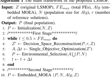
The main framework of the proposed large-scale multi-objective optimization framework (LSMOF) is presented in Algorithm 1. To begin with, the population of the embedded MOEA is initialized. Then a two-stage strategy is applied, where the first stage aims to find several quasi-optimal so-lutions near the PS and the second stage spreads them over the approximate PS uniformly. At the first stage, the decision space is reconstructed with the assistance of population P, and a single-objective optimization problem (SOP) Z′ is formulated; then, a single-objective optimizer (e.g. the differ-ential evolution (DE) algorithm [36]) is used to optimize Z′. The above decision space reconstruction and single-objective optimization repeat until the maximum number of function FEs is reached. For simplicity, we allocate 50% of the whole FEs to each stage. At the second stage, the original LSMOP is optimized by the embedded MOEA with the populationP obtained at the first stage. Note that the LSMOF framework shares the same environmental selection operator with the embedded MOEA, and thus we will not enter the details of it. In the following subsections, we will introduce the other two main components in Algorithm 1, i.e., decision space reconstruction and single-objective optimization.

A. Decision Space Reconstruction

Decision space reconstruction is a crucial component of the proposed LSMOF (Step 4 in Algorithm 1), which transforms an LSMOP into a series of MOPs with relatively small-scale weight variables to improve the efficiency of the algorithm, where the decision space of each constructed MOP is a subspace of the original LSMOP. To be specific, the proposed decision space reconstruction consists of two steps: the bi-direction weight variable association and the weight variable based subproblem construction.

1) Weight Variable Association: To guide the search of the algorithm towards the PS, a set of well converged and

Algorithm 1 The main framework of the proposed LSMOF.

Input: Z (original LSMOP),F Emax (total FEs), Alg (em-bedded MOEA), N (population size forAlg),r(number of reference solutions).

Output: P (final population). 1: P ←Initialization(N, Z)

2: /***********First Stage***********/ 3: while t≤0.5×F Emax do

4: Z′←Decision Space Reconstruction(P, r, Z) 5: A,∆t←Single Objective Optimization(Z′) 6: P ←Environmental Selection(A∪P, N)

7: t←t+ ∆t 8: end

9: /*********Second Stage*********/ 10: P ←Embedded MOEA (P, N, Alg, Z)

uniformly distributed candidate solutions is used during the decision space reconstruction. For simplicity, we directly use the environmental selection in the embedded MOEA to select r solutions from the current population P as the reference solution set.

After the selection of reference solutions, each reference solution is associated with two direction vectors and two weight variables, which aims to specify the search directions in the decision space to guide the population towards the PS.

3DUHWRRSWLPDOVHW [ [

V

R

W

S S __ __ X X λ Y Y _{__ __}O O λ Y Y O Y X Y

Fig. 2: An example of the bi-directional weight variable association. In this example,s1 is a selected solution, oand t are the lower and upper boundary points, and p1 and p2 are intersections between the direction vectors and the

PS. Besides, two weight variablesλ11, λ12 and two direction

vectorsvl,vu are associated with this solution.

To illustrate the relationship among the reference solutions, the direction vectors, and the weight variables, an example is displayed in Fig. 2, where a reference solution s1 = (x1, . . . , xd) is located in a two-dimensional decision space. oand tare the lower and upper boundary points of X, and

(5)

s1, where

vl = s1−o (4)

vu = t−s1,

with lmax=||t−o|| denoting the maximum diagram length inX. Assume pointsp1,p2 are intersections between vectors

vl,vu and the PS, and the distances from oto p1 and from

ttop2areλ11 andλ12respectively, the values ofp1andp2

can be calculated as p1 = o+λ11 vl ||vl|| lmax (5) p2 = t−λ12 vu ||vu|| lmax,

where the weight variables are ranged in [0,0.5] instead of

[0,1]to avoid overlapping.

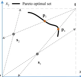
To be specific, each reference solution is associated with two bi-directional vectors instead of a uni-directional vector, which is out of two main considerations. First, the bi-directional vectors can enhance the population diversity, thus reducing the possibility of the disjoint situation where there is no intersection between the direction vector and the PS. For instance, if the reference solution locates around the boundary of the PS or the PS locates around a corner of the decision space, the direction vector may disjoint with the PS, but the bi-directional vectors are more likely to have more than one intersections with the PS. Second, the bi-directional vectors can eliminate the nonuniform search caused by the divergence of the unidirectional vectors. To further illustrate the motiva-tion of the motivamotiva-tion of the proposed bi-direcmotiva-tional weight variable association strategy, an example is given in Fig. 3. Generally, it has better chance to locate the Pareto optimal solutions on the PS by applying the bi-directional vectors than the unidirectional vectors.

2) Subproblem Construction: Given a reference solution set with sizer, once each reference solution is associated with two direction vectors and two weight variables, a total number of

2rsubproblems can be constructed in the reconstructed deci-sion space. Taking the first reference solution xfor example, two subproblems can be constructed as follows:

z11(λ11) = F(o+λ11 vl ||vl|| lmax) (6) z12(λ12) = F(t−λ12 vu ||vu|| lmax),

whereλ11,λ12 are two one-dimensional weight variables,vl, vu are the reference directions calculated by (4), and o, t, lmax are elements explained in (5). The constructed subprob-lems areZ′(Λ)={z11(λ11), z12(λ12),. . . ,zr1(λr1),zr2(λr2)},

where the weight vectorΛ={λ11, λ12, . . . , λr1, λr2} is in the

reconstructed decision space.

It is worth noting that there are two main differences between our proposed decision space reconstruction and the problem transformation in WOF. First, while the decision variables in WOF are divided using grouping techniques, the decision variables in the proposed LSMOF are controlled by the weight variables and optimized as a whole. On one hand, it can explicitly save the computational cost of variable analysis;

[

V V R W S S 3DUHWRRSWLPDOVHW

(a) Illustration of the proposed bi-directional weight variable association strategy in a 2D decision space.

[

R W 3DUHWRRSWLPDOVHW

V

(b) Illustration of the uni-directional weight variable association strategy in a 2D decision space.

Fig. 3: An example illustrating the motivation of the proposed bi-directional weight variable association strategy in a 2D decision space. s2,s3 are the reference solutions, p3, p4 are the intersections, and o,t are the lower and upper boundary points respectively.

on the other hand, it can implicitly take the interdependence between the pairwise decision variables into consideration during the evolution. Second, while the direction vectors in WOF are unidirectional, those in the proposed LSMOF are bidirectional. In general, the coverage of the bi-directional search in LSMOF is larger than that of WOF, which enhances the exploration ability of the algorithm and maintains better population diversity.

B. Single-Objective Optimization

Once the decision space is reconstructed, the optimization of the decision vector x in the original decision space is transformed to the optimization of the weight vector Λ in the reconstructed decision space Correspondingly, the new

(6)

optimization problem can be formulated as:

Maximize G(Λ) =H(Z′(Λ)) (7) subject to Λ∈ ℜ2r_,

where H is a function to assess the quality of 2r multi-objective solutions, andH can be any performance indicator, e.g., the hypervolume (HV) indicator [37] as adopted in this work. In the following, we will first demonstrate the proposed fitness assignment strategy for the evaluation of (7), and then elaborate the details of the DE based single-objective optimization in our proposed LSMOF.

1) Fitness Assignment: As given by the pseudo code of the fitness assignment procedure in Algorithm 2, the fitness of a weight vector in the reconstructed decision space can be calculated by two main stages. At the first stage, the objective vector in accordance with the weight vector Λ are calculated (Step 1 to Step 6). Then, at the second stage, the fitness value of the objective vector is calculated using the hpyervolume indicator. In this way, the algorithm is able to return a scalar value as the fitness of the reconstructed decision vector Λ.

Algorithm 2 The fitness assignment strategy in LSMOF.

Input: Λ (weight vector), R (reference solution set), P (current population).

Output: f it(Λ)(fitness value ofΛ).

1: N ad←Calculate the nadir point ofP in objective space 2: fori←1 :rdo

3: vl,vu←Calculate direction vectors using (4)

4: p1,p2 ← Calculate the weight variable associated solutions using (5)

5: zi1(λi1), zi2(λi2) ← Calculate the objective vectors

using (6) 6: end

7: Z′(Λ)← {z11(λ11), z12(λ12), . . . , zr1(λr1), zr2(λr2)}

8: f it(Λ)←Hypervolume(Z′(Λ), N ad)

2) Differential Evolution: Given the the decision space re-construction and the fitness assignment, the proposed LSMOF is expected to perform single-objective optimization of the weight variables in the reconstructed decision space. For simplicity, we adopt the widely used differential evolution (DE) [38] as the single-objective optimizers in this work.

The details of the DE based single-objective optimization are presented in Algorithm 3. In this algorithm, a set of weight vectors PΛ are first initialized in range [0,0.5]as defined in

(5), and their fitness values are calculated using Algorithm 2. For each weight vector Λi in PΛ, three different weight

vectors are randomly selected fromPΛ to form a trail vector a for crossover, wherea is associated with the weight vector to generate an offspring b according to a probability rate CR. If the fitness of offspring a is better than that of Λi, the weight vector Λi is replaced by b. The reproduction and replacement procedures repeat for a number ofgiterations, and all the candidate solutions generated during the evolution of the weight vectors are merged into the archive A, which will be used as the initial population of the embedded MOEA at Step 10 in Algorithm 1.

Algorithm 3 The DE based single-objective optimization in LSMOF

Input: N I (population size of DE),g (maximum number of iterations), CR(cross constant), Fm(scaling factor).

Output: A (population),∆t (number of FEs). 1: ∆t←0

2: PΛ← {Λ1, . . . ,ΛN I} /*Initialization*/

3: f it(Λ1),. . . ,f it(ΛN I) ← Calculate the fitnesses of ele-ments inPΛ using Algorithm 2

4: A← Collet the generated candidate solutions during the fitness assignment

5: ∆t←∆t+|A|/*|A| denotes the element size ofA*/ 6: forr←1 :g do

7: fori←1 :N I do

8: c1, c2, c3←Randomly select three indices in[1, N I]

9: a←Λc1+Fm(Λc2−Λc3)

10: forj←1 :|Λ1| do

11: if randj[0,1)≤CR orj=jrand then

12: bi←Choose the jth element ofΛi

13: else

14: bi←Choose the jth element ofa

15: end

16: end

17: f it(b)←Calculate b’s fitness using Algorithm 2 18: A′ ←Collet the generated candidate solutions during

the fitness assignment 19: ∆t←∆t+|A′| 20: if f it(b)≥f it(Λi) then 21: Λi←b 22: end 23: A←A∪A′ 24: end 25: end

IV. EMPIRICALSTUDIES

To empirically investigate the performance of the pro-posed LSMOF framework, four representative MOEAs, name-ly, NSGA-II [7], MOEA/D-DE [11], SMS-EMOA [13], and CMOPSO [27], are embedded into LSMOF and compared with their original versions on nine test problems from the LSMOP test suite [14]. Here we adopt these four algorithms as they represent different types of MOEAs as discussed in Section I, and the embedding of these algorithms could reveal the potential advantages of our proposed LSMOF. Then, two state-of-the-art large-scale MOEAs, namely, WOF [26]1 and MOEA/DVA [34], are also compared with our proposed LSMOF2_.

In the remainder of this section, we first present a brief introduction to the adopted performance indicator, then we give the parameter settings of the compared algorithms and our proposed LSMOF. Afterwards, each algorithm is run for 20 times on each test problem independently, and the Wilcoxon rank sum test [41] is adopted to compare the results obtained

1_{The implementation of WOF is adapted from the codes available at http:}

//www.is.ovgu.de/Team/Heiner+Zille.html.

2_{More experimental results on test problems selected from DTLZ [39] and}

(7)

by the proposed LSMOF and the compared algorithms at a significance level of 0.05. Symbols ‘+’, ‘−’, and ‘≈’ indicate the compared algorithm is significantly outperformed, significantly underperformed, and statistically tied by LSMOF.

A. Performance Indicator

In the experiments, a widely used performance indicator, the inverted generational distance (IGD) [42], is adopted for evaluating the performance of the compared algorithms.

Suppose that P∗ is a set of evenly distributed reference points on the PF and Ωis the set of obtained non-dominated solutions, IGD is defined as follows:

IGD(P∗,Ω) = ∑

x∈P∗dis(x,Ω)

|P∗| , (8)

where dis(x,Ω)is the minimum Euclidean distance between

xand points inΩand|P∗|the number of elements inP∗. A smaller value of IGD will indicate a better performance of the algorithm. In this work, the size of P∗ is set to 10000 (or a close number) for the IGD calculations.

B. Experimental Settings

For fair comparisons, we adopt the recommended parameter settings for the compared algorithms that have achieved the best performance as reported in the literature. All the com-pared algorithms are implemented in PlatEMO [43].3

1) Reproduction Operators. In this work, simulated binary crossover (SBX) [44] and polynomial mutation (PM) [45] are adopted in the compared algorithms for offspring genera-tion in NSGA-II and SMS-EMOA. The distribugenera-tion index of crossover is set to nc=20 and the distribution index of muta-tion is set to nm=20, as recommended in [4]. The crossover probability pc is set to 1.0 and the mutation probability pm is set to 1/D, where D is the number of decision variables. In MOEA/D-DE and MOEA/DVA, differential evolution (DE) operator [36] and PM are used for offspring generation, where the control parameters are set toCR=1,F=0.5,pm=1/d, and η=20 as recommended in [11]. As for CMOPSO, the particle swarm operator [46] and PM are used, where parameters R1

andR2 are randomly selected from[0,1]withγ set to 10 as

recommended in [27].

2) Population Size.The population size is set to 100 for test instances with two objectives and 105 for test instances with three objectives.

(3) Specific Parameter Settings in Each Algorithm. In MOEA/D-DE, the neighborhood size T is set to 20, the probability of choosing parents locally δ is set to 0.9, and the maximum number of solutions replaced by each offspring nr is set to 2. In WOF, the number of function evaluations for the optimization of each original problemt1is set to 500,

and for the transferred problem, t2 is set to 250, parameter

q is set to 3, the number of groups γ is set to 4, and the ordered grouping is adopted as the grouping method [26]. In MOEA/DVA, the number of sampling solutions to recognize

3_The _source _code _of _PlatEMO _can _be _downloaded _from:

http://bimk.ahu.edu.cn/index.php?s=/Index/Software/index.html.

the control property of decision variableN CAis set to 20, and the maximum number of tries required to judge the interaction between two variablesN IAis set to 6 [34].

In the proposed LSMOF, the number of reference solutions r is set to 10, the population size for single-objective opti-mization problem N I is set to 30, and the mutation factor Fmin DE is set to 0.8.

(4) Termination Condition. A total number of 50000 func-tion evaluafunc-tions is adopted as the terminafunc-tion condifunc-tion for all the test instances.

C. General Performance

To investigate the effect of LSMOF on different MOEAs, four representative algorithms, i.e., NSGA-II, MOEA/D-DE, SMS-EMOA, and CMOPSO, are embedded into the proposed framework. Pairwise comparisons are conducted between the heuristic algorithm and its LSMOF version in terms of both solution quality and algorithm runtime. The experimental results obtained by these compared algorithms are displayed in Table I, where LS-Algdenotes the LSMOF with algorithm Alg embedded.

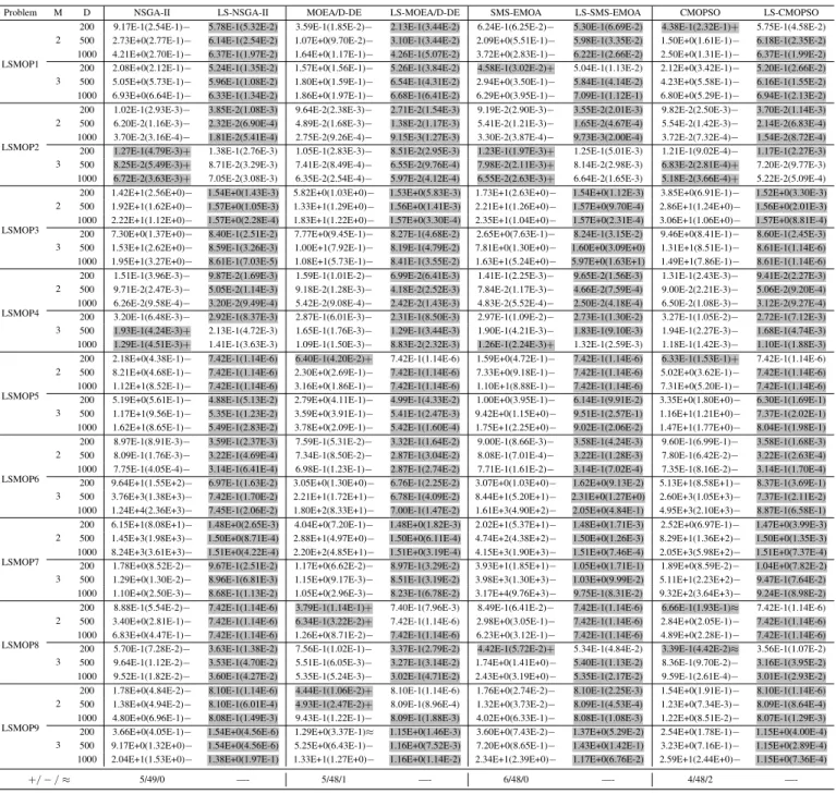
In Table I, the four original algorithms are outperformed by the LSMOF-based versions on 48 out of 56 test instances. On one hand, NSGA-II outperforms LS-NSGA-II on tri-objective LSMOP2 and LSMOP4, MOEA/D-DE mainly outperforms LS-MOEA/D-DE on 4 test instances with 200 and 500 de-cision variables, SMS-EMOA outperforms LS-SMS-EMOA on tri-objective LSMOP2 and two test instances with 200 decision variables, and CMOPSO has achieved two better results on LSMOP2 and other two test instances with 200 decision variables compared with LS-CMOPSO. Besides, most of the best results are achieved by LS-MOEA/D-DE, totaling 31 out of 56 test instances. It is mainly attributed to the fact that the LSMOP problems are designed with decision variables linked on the PSs, and the MOEA/D-DE is exactly tailored for solving problems with complicated PSs. All in all, the pairwise comparisons have demonstrated the optimization performance of our proposed LSMOF.

In addition to the pairwise comparison differences among the 56 test instances, a more significant performance improve-ment achieved by LSMOF can be observed on test instances with a larger number of decision variables ( e.g.LSMOP7, LSMOP8, and LSMOP9), which indicates the good scalability of LSMOF.

D. Computational Efficiency

Since one important motivation of our proposed LSMOF is to accelerate large-scale multi-objective optimization for enhancing the computational efficiency, we will further inves-tigate the convergence speed and computational speed of the compared algorithms by two experiments.

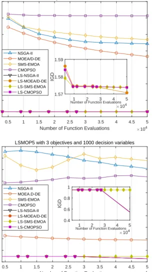
1) Convergence Speed: The convergence profiles of the eight compared algorithms on LSMOP3 and LSMOP5 with 1000 decision variables are displayed in Fig. 4.

As can be observed in Fig. 4, while the original algorithms converge slowly and thus have failed to converge to an acceptable accuracy level by the end of the evolution, by

(8)

TABLE I: The Statics of IGD Results Obtained by Eight Compared Algorithms on 54 Test Instances from LSMOP Test Suite. The Best Results in Each Two Columns are Highlighted.

Problem M D NSGA-II LS-NSGA-II MOEA/D-DE LS-MOEA/D-DE SMS-EMOA LS-SMS-EMOA CMOPSO LS-CMOPSO

LSMOP1 2

200 9.17E-1(2.54E-1)− 5.78E-1(5.32E-2) 3.59E-1(1.85E-2)− 2.13E-1(3.44E-2) 6.24E-1(6.25E-2)− 5.30E-1(6.69E-2) 4.38E-1(2.32E-1)+ 5.75E-1(4.58E-2) 500 2.73E+0(2.77E-1)− 6.14E-1(2.54E-2) 1.07E+0(9.70E-2)− 3.10E-1(3.44E-2) 2.09E+0(5.51E-1)− 5.98E-1(3.35E-2) 1.50E+0(1.61E-1)− 6.18E-1(2.35E-2) 1000 4.21E+0(2.70E-1)− 6.37E-1(1.97E-2) 1.64E+0(1.17E-1)− 4.26E-1(5.07E-2) 3.72E+0(2.83E-1)− 6.22E-1(2.66E-2) 2.50E+0(1.31E-1)− 6.37E-1(1.99E-2) 3

200 2.08E+0(2.12E-1)− 5.24E-1(1.35E-2) 1.57E+0(1.56E-1)− 5.26E-1(3.84E-2) 4.58E-1(3.02E-2)+ 5.04E-1(1.13E-2) 2.12E+0(3.42E-1)− 5.20E-1(2.66E-2) 500 5.05E+0(5.73E-1)− 5.96E-1(1.08E-2) 1.80E+0(1.59E-1)− 6.54E-1(4.31E-2) 2.94E+0(3.50E-1)− 5.84E-1(4.14E-2) 4.23E+0(5.58E-1)− 6.16E-1(1.55E-2) 1000 6.93E+0(6.64E-1)− 6.33E-1(1.34E-2) 1.86E+0(1.97E-1)− 6.68E-1(6.41E-2) 6.29E+0(3.95E-1)− 7.09E-1(1.12E-1) 6.80E+0(5.29E-1)− 6.94E-1(2.13E-2)

LSMOP2 2

200 1.02E-1(2.93E-3)− 3.85E-2(1.08E-3) 9.64E-2(2.38E-3)− 2.71E-2(1.54E-3) 9.19E-2(2.90E-3)− 3.55E-2(2.01E-3) 9.82E-2(2.50E-3)− 3.70E-2(1.14E-3) 500 6.20E-2(1.16E-3)− 2.32E-2(6.90E-4) 4.89E-2(1.68E-3)− 1.38E-2(1.17E-3) 5.41E-2(1.21E-3)− 1.65E-2(4.67E-4) 5.54E-2(1.42E-3)− 2.14E-2(6.83E-4) 1000 3.70E-2(3.16E-4)− 1.81E-2(5.41E-4) 2.75E-2(9.26E-4)− 9.15E-3(1.27E-3) 3.30E-2(3.87E-4)− 9.73E-3(2.00E-4) 3.72E-2(7.32E-4)− 1.54E-2(8.72E-4) 3

200 1.27E-1(4.79E-3)+ 1.38E-1(2.76E-3) 1.05E-1(2.83E-3)− 8.51E-2(2.95E-3) 1.23E-1(1.97E-3)+ 1.25E-1(5.01E-3) 1.21E-1(9.02E-4)− 1.17E-1(2.27E-3) 500 8.25E-2(5.49E-3)+ 8.71E-2(3.29E-3) 7.41E-2(8.49E-4)− 6.55E-2(9.76E-4) 7.98E-2(2.11E-3)+ 8.14E-2(2.98E-3) 6.83E-2(2.81E-4)+ 7.20E-2(9.77E-3) 1000 6.72E-2(3.63E-3)+ 7.05E-2(3.08E-3) 6.35E-2(2.54E-4)− 5.97E-2(4.12E-4) 6.55E-2(2.63E-3)+ 6.64E-2(1.65E-3) 5.18E-2(3.66E-4)+ 5.22E-2(5.09E-4)

LSMOP3 2

200 1.42E+1(2.56E+0)− 1.54E+0(1.43E-3) 5.82E+0(1.03E+0)− 1.53E+0(5.83E-3) 1.73E+1(2.63E+0)− 1.54E+0(1.12E-3) 3.85E+0(6.91E-1)− 1.52E+0(3.30E-3) 500 1.92E+1(1.62E+0)− 1.57E+0(1.05E-3) 1.33E+1(1.29E+0)− 1.56E+0(1.41E-3) 2.21E+1(1.26E+0)− 1.57E+0(9.70E-4) 2.86E+1(1.24E+0)− 1.56E+0(2.01E-3) 1000 2.22E+1(1.12E+0)− 1.57E+0(2.28E-4) 1.83E+1(1.22E+0)− 1.57E+0(3.30E-4) 2.35E+1(1.04E+0)− 1.57E+0(2.31E-4) 3.06E+1(1.06E+0)− 1.57E+0(8.81E-4) 3

200 7.30E+0(1.37E+0)− 8.40E-1(2.51E-2) 7.77E+0(9.45E-1)− 8.27E-1(4.68E-2) 2.65E+0(7.63E-1)− 8.24E-1(3.15E-2) 9.46E+0(8.41E-1)− 8.60E-1(2.45E-3) 500 1.53E+1(2.62E+0)− 8.59E-1(3.26E-3) 1.00E+1(7.92E-1)− 8.19E-1(4.79E-2) 7.81E+0(1.30E+0)− 1.60E+0(3.09E+0) 1.31E+1(8.51E-1)− 8.61E-1(1.14E-6) 1000 1.95E+1(3.27E+0)− 8.61E-1(7.03E-5) 1.08E+1(5.73E-1)− 8.41E-1(3.55E-2) 1.63E+1(5.24E+0)− 5.97E+0(1.63E+1) 1.49E+1(7.86E-1)− 8.61E-1(1.14E-6)

LSMOP4 2

200 3.20E-1(6.48E-3)− 2.92E-1(8.37E-3) 2.87E-1(6.01E-3)− 2.31E-1(8.50E-3) 2.97E-1(1.09E-2)− 2.73E-1(1.30E-2) 3.27E-1(1.05E-2)− 2.72E-1(7.12E-3) 500 1.93E-1(4.24E-3)+ 2.13E-1(4.72E-3) 1.65E-1(1.76E-3)− 1.29E-1(3.44E-3) 1.90E-1(4.21E-3)− 1.83E-1(9.10E-3) 1.94E-1(2.27E-3)− 1.68E-1(4.74E-3) 1000 1.29E-1(4.51E-3)+ 1.41E-1(3.63E-3) 1.09E-1(1.50E-3)− 8.83E-2(2.32E-3) 1.26E-1(2.24E-3)+ 1.32E-1(2.59E-3) 1.18E-1(1.42E-3)− 1.10E-1(1.88E-3)

LSMOP5 2

200 2.18E+0(4.38E-1)− 7.42E-1(1.14E-6) 6.40E-1(4.20E-2)+ 7.42E-1(1.14E-6) 1.59E+0(4.72E-1)− 7.42E-1(1.14E-6) 6.33E-1(1.53E-1)+ 7.42E-1(1.14E-6) 500 8.21E+0(4.68E-1)− 7.42E-1(1.14E-6) 2.30E+0(2.69E-1)− 7.42E-1(1.14E-6) 7.33E+0(9.18E-1)− 7.42E-1(1.14E-6) 5.02E+0(3.62E-1)− 7.42E-1(1.14E-6) 1000 1.12E+1(8.52E-1)− 7.42E-1(1.14E-6) 3.16E+0(1.86E-1)− 7.42E-1(1.14E-6) 1.10E+1(8.88E-1)− 7.42E-1(1.14E-6) 7.31E+0(5.20E-1)− 7.42E-1(1.14E-6) 3

200 5.19E+0(5.61E-1)− 4.88E-1(5.13E-2) 2.79E+0(4.11E-1)− 4.99E-1(4.33E-2) 1.00E+0(3.95E-1)− 6.14E-1(9.91E-2) 3.35E+0(1.80E+0)− 6.30E-1(1.69E-1) 500 1.17E+1(9.56E-1)− 5.35E-1(1.23E-2) 3.59E+0(3.91E-1)− 5.41E-1(2.47E-3) 9.42E+0(1.15E+0)− 9.51E-1(2.57E-1) 1.16E+1(1.21E+0)− 7.37E-1(2.02E-1) 1000 1.62E+1(8.65E-1)− 5.49E-1(2.83E-2) 3.78E+0(2.09E-1)− 5.42E-1(1.60E-4) 1.75E+1(2.25E+0)− 9.02E-1(2.06E-2) 1.47E+1(1.77E+0)− 8.04E-1(1.98E-1)

LSMOP6 2

200 9.64E+1(1.55E+2)− 6.97E-1(1.63E-2) 3.05E+0(1.30E+0)− 6.76E-1(2.25E-2) 3.07E+0(1.03E+0)− 1.62E+0(9.13E-2) 5.13E+1(8.58E+1)− 8.37E-1(3.69E-1) 500 3.76E+3(1.38E+3)− 7.42E-1(1.70E-2) 2.21E+1(1.72E+1)− 6.78E-1(4.09E-2) 8.44E+1(5.20E+1)− 2.31E+0(1.27E+0) 2.60E+3(1.05E+3)− 7.37E-1(2.11E-2) 1000 1.24E+4(2.36E+3)− 7.45E-1(2.06E-2) 1.80E+2(8.33E+1)− 7.00E-1(1.47E-2) 1.61E+3(4.90E+2)− 2.05E+0(4.84E-1) 4.95E+3(2.10E+3)− 8.87E-1(6.58E-1)

LSMOP7 2

200 6.15E+1(8.08E+1)− 1.48E+0(2.65E-3) 4.04E+0(7.20E-1)− 1.48E+0(1.82E-3) 2.02E+1(5.37E+1)− 1.48E+0(1.71E-3) 2.52E+0(6.97E-1)− 1.47E+0(3.99E-3) 500 1.45E+3(1.98E+3)− 1.50E+0(8.71E-4) 2.88E+1(4.97E+0)− 1.50E+0(6.11E-4) 4.74E+2(4.38E+2)− 1.50E+0(1.26E-3) 8.29E+1(1.36E+2)− 1.50E+0(1.35E-3) 1000 8.24E+3(3.61E+3)− 1.51E+0(4.22E-4) 2.20E+2(4.85E+1)− 1.51E+0(3.19E-4) 4.15E+3(1.90E+3)− 1.51E+0(7.46E-4) 2.05E+3(5.98E+2)− 1.51E+0(7.37E-4) 3

200 1.78E+0(8.52E-2)− 9.67E-1(2.51E-2) 1.17E+0(6.62E-2)− 8.97E-1(3.29E-2) 3.93E+1(1.85E+1)− 1.05E+0(1.71E-1) 1.89E+0(8.59E-2)− 1.04E+0(7.82E-2) 500 1.29E+0(1.30E-2)− 8.96E-1(6.81E-3) 1.15E+0(9.17E-3)− 8.51E-1(3.19E-2) 3.98E+3(1.30E+3)− 1.03E+0(9.99E-2) 5.11E+1(2.23E+2)− 9.47E-1(7.64E-2) 1000 1.10E+0(2.50E-3)− 8.68E-1(1.13E-2) 1.05E+0(2.96E-3)− 8.23E-1(6.78E-2) 3.17E+4(9.76E+3)− 9.75E-1(8.31E-2) 9.32E+2(3.64E+3)− 9.24E-1(8.98E-2)

LSMOP8 2

200 8.88E-1(5.54E-2)− 7.42E-1(1.14E-6) 3.79E-1(1.14E-1)+ 7.40E-1(7.96E-3) 8.49E-1(6.41E-2)− 7.42E-1(1.14E-6) 6.66E-1(1.93E-1)≈ 7.42E-1(1.14E-6) 500 3.40E+0(2.81E-1)− 7.42E-1(1.14E-6) 6.34E-1(3.22E-2)+ 7.42E-1(1.14E-6) 2.98E+0(3.05E-1)− 7.42E-1(1.14E-6) 2.84E+0(2.05E-1)− 7.42E-1(1.14E-6) 1000 6.83E+0(4.47E-1)− 7.42E-1(1.14E-6) 1.26E+0(8.71E-2)− 7.42E-1(1.14E-6) 6.23E+0(3.12E-1)− 7.42E-1(1.14E-6) 4.89E+0(2.28E-1)− 7.42E-1(1.14E-6) 3

200 5.70E-1(7.28E-2)− 3.63E-1(1.38E-2) 7.56E-1(1.02E-1)− 3.37E-1(2.79E-2) 4.42E-1(5.72E-2)+ 5.34E-1(4.84E-2) 3.39E-1(4.42E-2)≈ 3.56E-1(1.07E-2) 500 9.64E-1(1.12E-2)− 3.53E-1(4.70E-2) 5.51E-1(6.05E-3)− 3.27E-1(3.14E-2) 1.74E+0(1.41E+0)− 5.40E-1(1.13E-2) 8.36E-1(9.70E-2)− 3.16E-1(3.95E-2) 1000 9.52E-1(1.82E-2)− 3.60E-1(4.27E-2) 5.35E-1(5.24E-3)− 3.02E-1(4.71E-2) 2.43E+0(3.19E+0)− 5.35E-1(2.17E-2) 9.59E-1(2.61E-4)− 3.01E-1(2.93E-2)

LSMOP9 2

200 1.78E+0(4.84E-2)− 8.10E-1(1.14E-6) 4.44E-1(1.06E-2)+ 8.10E-1(1.14E-6) 1.76E+0(2.74E-2)− 8.10E-1(2.25E-3) 1.54E+0(1.91E-1)− 8.10E-1(1.14E-6) 500 1.38E+0(4.94E-2)− 8.10E-1(6.01E-4) 4.93E-1(2.47E-2)+ 8.09E-1(8.96E-4) 1.32E+0(3.73E-2)− 8.09E-1(4.53E-4) 1.23E+0(7.34E-3)− 8.09E-1(8.64E-4) 1000 4.80E+0(6.96E-1)− 8.08E-1(1.49E-3) 9.43E-1(1.22E-1)− 8.09E-1(1.88E-3) 4.02E+0(6.33E-1)− 8.08E-1(1.08E-3) 1.22E+0(8.51E-2)− 8.07E-1(1.29E-3) 3

200 3.66E+0(4.05E-1)− 1.54E+0(4.56E-6) 1.29E+0(3.37E-1)≈ 1.15E+0(1.46E-3) 3.60E+0(7.43E-2)− 1.37E+0(5.29E-2) 2.54E+0(1.78E-1)− 1.15E+0(4.00E-4) 500 9.17E+0(1.32E+0)− 1.54E+0(4.56E-6) 5.25E+0(6.43E-1)− 1.16E+0(7.52E-3) 7.20E+0(8.65E-1)− 1.43E+0(1.42E-1) 3.23E+0(7.16E-1)− 1.15E+0(2.89E-4) 1000 2.04E+1(1.53E+0)− 1.38E+0(1.97E-1) 1.33E+1(1.27E+0)− 1.16E+0(1.14E-2) 2.34E+1(2.39E+0)− 1.17E+0(6.76E-2) 2.59E+1(2.44E+0)− 1.15E+0(7.36E-4)

+/−/≈ 5/49/0 —- 5/48/1 —- 6/48/0 —- 4/48/2

—-contrast, the LSMOF-based algorithms have already converged to a promising accuracy level at a very early stage of the evolution (i.e., before 5000 function evaluations). This has indicated the high computational efficiency of the convergence speed.

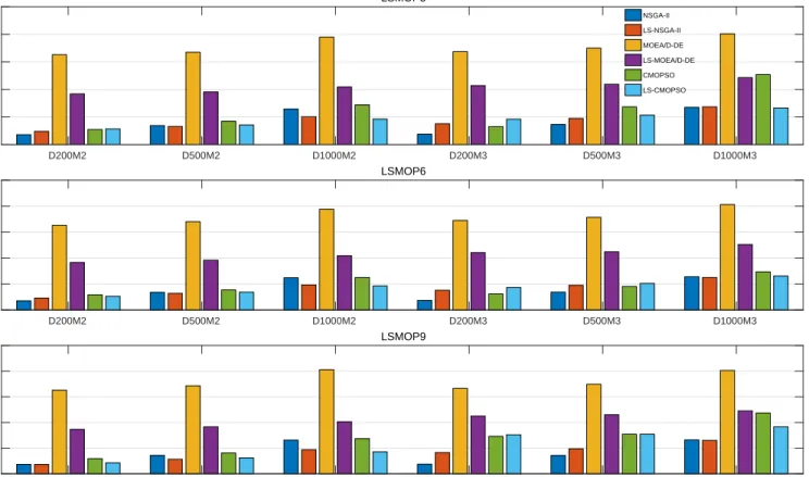
2) Computation Time: In order to investigate the compu-tation time of the proposed LSMOF, we display the aver-age computation time of the eight compared algorithms on LSMOP3, LSMOP6, and LSMOP9.

As shown in Fig. 5 and Fig. 6, our proposed LSMOF has accelerated the computation time of MOEA/D-DE and SMS-EMOA on all the test instances, especially for SMS-SMS-EMOA on tri-objective problems (with almost 50%computation time

reduced). As for NSGA-II and CMOPSO, LSMOF has saved little computational time on problems with 200 decision vari-ables but almost 1/3 computation time on problems with 500 and 1000 decision variables.

In conclusion, our proposed LSMOF is capable of reducing the computation time of MOEAs on large-scale multi-objective optimization, and the acceleration improvement is more signif-icant on LSMOPs with a larger number of decision variables, e.g, LSMOPs with more than 500 decision variables.

E. Comparisons with State-of-the-Arts

In this section, we compare our proposed LSMOF with another two state-of-the-art large-scale MOEAs, namely,

(9)

LSMOP3 D200M2 D500M2 D1000M2 D200M3 D500M3 D1000M3 0 10 20 30 40 50 Time(s) NSGA-II LS-NSGA-II MOEA/D-DE LS-MOEA/D-DE CMOPSO LS-CMOPSO LSMOP6 D200M2 D500M2 D1000M2 D200M3 D500M3 D1000M3 0 10 20 30 40 50 Time(s) LSMOP9 D200M2 D500M2 D1000M2 D200M3 D500M3 D1000M3 0 10 20 30 40 50 Time(s)

Fig. 5: The average computation time of NSGA-II, MOEA/D-DE, CMOPSO, and their LSMOF-based versions on LSMOP3, LSMOP6, and LSMOP9, where M denotes the number of objectives andD denotes the number of decision variables.

LSMOP3 D200M2 D500M2 D1000M2 D200M3 D500M3 D1000M3 0 500 1000 1500 Time(s) SMS-EMOA LS-SMS-EMOA LSMOP6 D200M2 D500M2 D1000M2 D200M3 D500M3 D1000M3 0 200 400 600 800 Time(s) LSMOP9 D200M2 D500M2 D1000M2 D200M3 D500M3 D1000M3 0 200 400 600 800 Time(s)

Fig. 6: The average computation time of SMS-EMOA and LS-SMS-EMOA on LSMOP3, LSMOP6, and LSMOP9, whereM denotes the number of objectives andD denotes the number of decision variables.

(10)

0.5 1 1.5 2 2.5 3 3.5 4 4.5 5

Number of Function Evaluations 104

0 5 10 15 20 25 30 35 IGD

LSMOP3 with 2 objectives and1000 decision variables

NSGA-II MOEA/D-DE SMS-EMOA CMOPSO LS-NSGA-II LS-MOEA/D-DE LS-SMS-EMOA LS-CMOPSO 1 2 3 4 5

Number of Function Evaluations 104 1.57 1.58 1.59 IGD 0.5 1 1.5 2 2.5 3 3.5 4 4.5 5

Number of Function Evaluations 104

0 2 4 6 8 10 12 14 16 18 20 IGD

LSMOP5 with 3 objectives and 1000 decision variables

NSGA-II MOEA.D-DE SMS-EMOA CMOPSO LS-NSGA-II LS-MOEA/D-DE LS-SMS-EMOA

LS-CMOPSO _{Number of Function Evaluations}1 2 3 4 5

104 0.4 0.6 0.8 1 IGD

Fig. 4: The convergence profiles of eight compared algorithms on bi-objective LSMOP3 and tri-objective LSMOP5 with 1000 decision variables.

MOEA/DVA and WOF, in terms of both optimization per-formance and computational efficiency. In both WOF and LSMOF, NSGA-II is embedded for a fair comparison. The statistics of IGD results achieved by MOEA/DVA, WOF-NSGA-II, and LS-NSGA-II are displayed in Table II.

As summarized in Table II, LS-NSGA-II has achieved 32 best results out of 54 test instances, WOF-NSGA-II has achieved 6 best results, and MOEA/DVA has achieved 5 best results. To be specific, LS-NSGA-II has achieved the best results mainly on LSMOP1, LSMOP3, LSMOP5, LSMOP6, LSMOP7, LSMOP8, and bi-objective LSMOP2 and LSMOP9; WOF-NSGA-II has achieved the best results mainly on LSMOP5 and tri-objective LSMOP9; meanwhile, MOEA/DVA has achieved the best results on tri-objective LSMOP2 and tri-objective LSMOP4.

It should be noted that MOEA/DVA has achieved some results far from the Pareto optimal fronts on LSMOP6 and bi-objective LSMOP7. This may be attributed to the failure of decision variables analysis, which has caused the significant performance degeneration.

TABLE II: The Statics of IGD Results Achieved by Three Compared Algorithms on 54 Test Instances from LSMOP Test Suite. The Best Result in Each Row is Highlighted.

Problem M D MOEA/DVA WOF-NSGA-II LS-NSGA-II

LSMOP1 2

200 8.66E+0(8.04E-1)− 6.30E-1(9.36E-2)− 5.78E-1(5.32E-2) 500 1.91E+1(1.00E+0)− 6.58E-1(6.11E-2)− 6.14E-1(2.54E-2) 1000 2.39E+1(7.84E-1)− 6.79E-1(4.22E-2)− 6.37E-1(1.97E-2) 3

200 6.26E+0(4.62E-1)− 6.95E-1(1.32E-1)− 5.24E-1(1.35E-2) 500 9.42E+0(2.89E-1)− 7.09E-1(8.36E-2)− 5.96E-1(1.08E-2) 1000 1.08E+1(3.22E-1)− 8.01E-1(7.05E-2)− 6.33E-1(1.34E-2) LSMOP2 2

200 1.51E-1(6.75E-4)− 7.46E-2(4.63E-4)− 3.85E-2(1.08E-3) 500 7.27E-2(2.30E-4)− 3.30E-2(3.91E-4)− 2.32E-2(6.90E-4) 1000 4.04E-2(3.87E-4)− 1.92E-2(3.40E-4)− 1.81E-2(5.41E-4) 3

200 1.23E-1(2.61E-3)+ 1.36E-1(3.84E-3)≈ 1.38E-1(2.76E-3) 500 7.89E-2(2.63E-3)+ 8.54E-2(3.82E-3)≈ 8.71E-2(3.29E-3) 1000 6.48E-2(2.46E-3)+ 7.00E-2(4.28E-3)≈ 7.05E-2(3.08E-3) LSMOP3 2

200 1.71E+1(1.30E+0)− 1.50E+0(6.88E-2)≈ 1.54E+0(1.43E-3) 500 2.87E+1(8.26E-1)− 1.57E+0(1.47E-3)− 1.57E+0(1.05E-3) 1000 3.36E+1(6.07E-1)− 1.58E+0(1.61E-3)− 1.57E+0(2.28E-4) 3

200 2.30E+1(3.53E+0)− 8.61E-1(3.38E-4)− 8.40E-1(2.51E-2) 500 3.60E+1(2.95E+0)− 8.61E-1(1.30E-4)− 8.59E-1(3.26E-3) 1000 4.02E+1(2.09E+0)− 8.61E-1(7.28E-4)≈ 8.61E-1(7.03E-5) LSMOP4 2

200 6.56E-1(9.76E-3)− 1.33E-1(1.51E-2)− 9.87E-2(1.69E-3) 500 5.44E-1(1.90E-3)− 8.74E-2(6.83E-3)− 5.05E-2(1.14E-3) 1000 4.61E-1(6.97E-4)− 5.99E-2(5.57E-3)− 3.20E-2(9.49E-4) 3

200 3.26E-1(2.31E-3)− 3.15E-1(9.10E-3)− 2.92E-1(8.37E-3) 500 1.94E-1(5.71E-4)+ 2.14E-1(6.87E-3)≈ 2.13E-1(4.72E-3) 1000 1.20E-1(1.96E-4)+ 1.39E-1(5.80E-3)≈ 1.41E-1(3.63E-3) LSMOP5 2

200 1.42E+1(6.21E-1)− 7.42E-1(1.14E-6)≈ 7.42E-1(1.14E-6) 500 2.09E+1(5.02E-1)− 7.42E-1(1.14E-6)≈ 7.42E-1(1.14E-6) 1000 2.41E+1(3.40E-1)− 7.42E-1(1.14E-6)≈ 7.42E-1(1.14E-6) 3

200 1.17E+1(9.27E-1)− 5.41E-1(1.02E-3)− 4.88E-1(5.13E-2) 500 1.70E+1(6.15E-1)− 5.41E-1(4.66E-5)− 5.35E-1(1.23E-2) 1000 1.91E+1(5.97E-1)− 5.41E-1(7.27E-5)≈ 5.49E-1(2.83E-2) LSMOP6 2

200 7.36E+2(6.12E+2)− 6.42E-1(7.36E-2)− 3.59E-1(2.37E-3) 500 2.24E+3(2.14E+3)− 7.33E-1(1.76E-1)− 3.22E-1(4.69E-4) 1000 2.99E+3(2.33E+3)− 6.82E-1(9.03E-4)− 3.14E-1(6.41E-4) 3

200 1.77E+4(3.58E+3)− 1.22E+0(3.15E-3)− 6.97E-1(1.63E-2) 500 3.05E+4(6.34E+3)− 1.29E+0(2.01E-3)− 7.42E-1(1.70E-2) 1000 3.68E+4(7.07E+3)− 1.31E+0(1.31E-3)− 7.45E-1(2.06E-2) LSMOP7 2

200 5.58E+4(6.03E+3)− 1.48E+0(2.34E-3)− 1.48E+0(2.65E-3) 500 1.06E+5(5.12E+3)− 1.51E+0(1.18E-3)− 1.50E+0(8.71E-4) 1000 1.33E+5(4.14E+3)− 1.51E+0(1.19E-3)− 1.51E+0(4.22E-4) 3

200 1.80E+0(3.92E-2)− 9.78E-1(4.70E-2)≈ 9.67E-1(2.51E-2) 500 1.27E+0(9.73E-3)− 9.48E-1(1.26E-1)− 8.96E-1(6.81E-3) 1000 1.10E+0(2.56E-3)− 9.23E-1(1.38E-1)− 8.68E-1(1.13E-2) LSMOP8 2

200 1.40E+1(8.86E-1)− 7.42E-1(1.14E-6)≈ 7.42E-1(1.14E-6) 500 2.11E+1(4.21E-1)− 7.42E-1(1.14E-6)≈ 7.42E-1(1.14E-6) 1000 2.39E+1(4.73E-1)− 7.42E-1(1.14E-6)≈ 7.42E-1(1.14E-6) 3

200 6.69E-1(1.07E-2)− 3.65E-1(4.56E-3)− 3.63E-1(1.38E-2) 500 6.51E-1(6.13E-3)− 3.55E-1(1.59E-2)− 3.53E-1(4.70E-2) 1000 6.49E-1(4.56E-3)− 3.56E-1(9.05E-3)+ 3.60E-1(4.27E-2) LSMOP9 2

200 2.26E+1(1.92E+0)− 8.10E-1(1.14E-6)≈ 8.10E-1(1.14E-6) 500 4.32E+1(1.36E+0)− 8.10E-1(3.21E-4)≈ 8.10E-1(6.01E-4) 1000 5.24E+1(1.03E+0)− 8.09E-1(4.10E-4)− 8.08E-1(1.49E-3) 3

200 6.70E+1(5.47E+0)− 7.74E-1(3.80E-1)+ 1.54E+0(4.56E-6) 500 1.15E+2(5.42E+0)− 8.21E-1(4.13E-1)+ 1.54E+0(4.56E-6) 1000 1.37E+2(3.51E+0)− 1.08E+0(4.00E-1)+ 1.38E+0(1.97E-1)

+/−/≈ 5/49/0 4/32/18

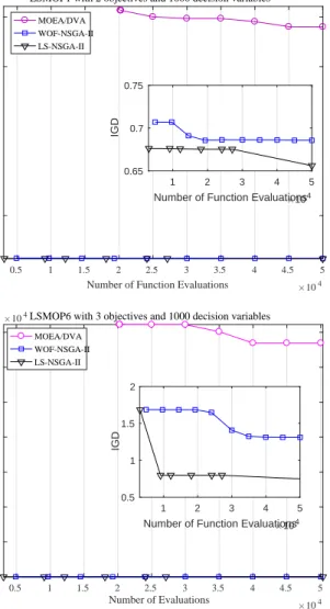
After comparing the performance of these three algorithms on LSMOPs, their convergence rates on bi-objective LSMOP1 and tri-objective LSMOP6 with 1000 decision variables are presented in Fig. 7, and the average computation time on LSMOP1 is displayed in Fig. 8. It can be observed from these two figures that LS-NSGA-II has the fastest convergence rate on those two test instances, while its computation time is similar to that of MOEA/DVA and WOF-NSGA-II.

In conclusion, the proposed LSMOF shows better optimiza-tion performance than that of MOEA/DVA and WOF on these LSMOPs with similar computational efficiencies, which has confirmed the competitiveness of LSMOF in comparison with the state-of-the-arts.

(11)

0.5 1 1.5 2 2.5 3 3.5 4 4.5 5 Number of Function Evaluations 104

5 20 25

IGD

LSMOP1 with 2 objectives and 1000 decision variables MOEA/DVA

WOF-NSGA-II LS-NSGA-II

1 2 3 4 5

Number of Function Evaluations104

0.65 0.7 0.75 IGD 0.5 1 1.5 2 2.5 3 3.5 4 4.5 5 Number of Evaluations ₁₀4 0.5 1 1.5 2 2.5 3 3.5 IGD

104LSMOP6 with 3 objectives and 1000 decision variables

MOEA/DVA WOF-NSGA-II LS-NSGA-II

1 2 3 4 5

Number of Function Evaluations104

0.5 1 1.5 2

IGD

Fig. 7: The convergence rates of three compared algorithms on bi-objective LSMOP1 and tri-objective LSMOP6 with 1000 decision variables. LSMOP1 D200M2 D500M2 D1000M2 D200M3 D500M3 D1000M3 0 2 4 6 8 10 12 14 Time(s) MOEA/DVA WOF-NSGA-II LS-NSGA-II

Fig. 8: The average computation time of MOEA/DVA, WOF-NSGA-II and LS-WOF-NSGA-II on LSMOP1, whereM denotes the number of objectives and D denotes the number of decision variables.

V. CONCLUSION

In this work, we have proposed a general framework for large-scale multi-objective optimization, termed LSMOF. The proposed LSMOF adopts a two-stage strategy, where the first stage conducts the decision space reconstruction for obtaining a set of quash-optimal solutions near the PS, and the second stage spreads these solutions over the approximate PS uni-formly by an embedded MOEA.

At the first stage of the proposed LSMOF, the decision space is first reconstructed by associating a set of reference solutions with a set of weight variables in the decision space. Then, a series of subproblems are constructed by taking the weight variables as the input, where each weight variable is aimed at tracking a specific point on the PS. The differential evolution algorithm is adopted to optimize the subproblems as a single-objective problem by using an indicator based fitness assignment strategy, and the candidate solutions obtained therein are used as the initial population of the embedded MOEA at the second stage.

To assess the performance of the proposed LSMOF, a variety of empirical comparisons have been conducted on a set of LSMOPs. The general performance of our proposed LSMOF is tested by embedding four MOEAs, namely, NSGA-II, MOEA/D-DE, SMS-EMOA, and CMOPSO into it. The statistical results indicate that LSMOF has accelerated the convergence speed and saved computation time of the em-bedded algorithms on most of the test instances, and more importantly, the performance of the MOEAs has been also been significantly improved. The second experiment assesses the performance of the proposed LSMOF in comparison with two state-of-the-art large-scale MOEAs, namely, MOEA/DVA and WOF. The superiority of the proposed LSMOF over the other two algorithms is verified by the experimental results.

The proposed LSMOF has shown good potential in large-scale multi-objective optimization. The decision space recon-struction reduces the dimensionality of the large-scale problem and guide the population towards the PS. Moreover, the update of the reference solutions and the dynamic decision space reconstruction enables the tracking of the PS adaptively. Future work on developing more efficient decision space reconstruction method is highly desirable. It is also of interest to extend our proposal to real-world LSMOPs with more decision variables by parallel (e.g. GPU-based) computing.

ACKNOWLEDGMENT

Part of the work was supported in part by National Nat-ural Science Foundation of China (61320106005, 61502004, 61502001, 61772214, and 61672033), in part by the Innova-tion Scientists and Technicians Troop ConstrucInnova-tion Projects of Henan Province (154200510012), and in part by an EPSRC grant (No. EP/M017869/1).

REFERENCES

[1] A. Ponsich, A. L. Jaimes, and C. A. C. Coello, “A survey on mul-tiobjective evolutionary algorithms for the solution of the portfolio optimization problem and other finance and economics applications,” IEEE Transactions on Evolutionary Computation, vol. 17, pp. 321–344, 2013.

(12)

[2] H. Ishibuchi and T. Murata, “Multiobjective genetic local search algo-rithm and its application to flowshop scheduling,”IEEE Transactions on Systems, Man, and Cybernetics-Part C, vol. 28, no. 3, pp. 392–403, 1998.

[3] Y. Tian, H. Wang, X. Zhang, and Y. Jin, “Effectiveness and efficiency of non-dominated sorting for evolutionary multi-and many-objective optimization,”Complex&Intelligent Systems, vol. 3, pp. 247–263, 2017. [4] K. Deb, Multi-objective optimization using evolutionary algorithms.

John Wiley & Sons, 2001, vol. 16.

[5] R. Cheng, Y. Jin, M. Olhofer, and B. Sendhoff, “A reference vector guided evolutionary algorithm for many-objective optimization,”IEEE Transactions on Evolutionary Computation, vol. 20, pp. 773–791, 2016. [6] A. Zhou, B.-Y. Qu, H. Li, S.-Z. Zhao, P. N. Suganthan, and Q. Zhang, “Multiobjective evolutionary algorithms: A survey of the state of the art,”Swarm and Evolutionary Computation, vol. 1, no. 1, pp. 32–49, 2011.

[7] K. Deb, A. Pratap, S. Agarwal, and T. Meyarivan, “A fast and elitist multi-objective genetic algorithm: NSGA-II,” IEEE Transactions on Evolutionary Computation, vol. 6, pp. 182–197, 2002.

[8] M. M. K. Deb and S. Mishra, “Evaluating theϵ-domination based multi-objective evolutionary algorithm for a quick computation of pareto-optimal solutions,”Evolutionary Computation, vol. 13, no. 4, pp. 501– 525, 2005.

[9] E. Zitzler, M. Laumanns, L. Thiele et al., “SPEA2: Improving the strength Pareto evolutionary algorithm for multiobjective optimization,” inEurogen, vol. 3242, no. 103, 2001, pp. 95–100.

[10] Q. Zhang and H. Li, “MOEA/D: A multiobjective evolutionary algorithm based on decomposition,”IEEE Transactions on Evolutionary Compu-tation, vol. 11, pp. 712–731, 2007.

[11] H. Li and Q. Zhang, “Multiobjective optimization problems with com-plicated Pareto sets, MOEA/D and NSGA-II,” IEEE Transactions on Evolutionary Computation, vol. 13, pp. 284–302, 2009.

[12] Y. Tian, X. Zhang, R. Cheng, and Y. Jin, “A multi-objective evolutionary algorithm based on an enhanced inverted generational distance metric,” in2016 IEEE Congress on Evolutionary Computation (CEC). IEEE, 2016, pp. 5222–5229.

[13] N. Beume, B. Naujoks, and M. Emmerich, “SMS-EMOA: Multiobjec-tive selection based on dominated hypervolume,”European Journal of Operational Research, vol. 181, no. 3, pp. 1653–1669, 2007. [14] R. Cheng, Y. Jin, M. Olhofer, and B. Sendhoff, “Test problems for

large-scale multiobjective and many-objective optimization,”IEEE Transac-tions on Cybernetics, vol. 47, pp. 4108 – 4121, 2017.

[15] L. Parsons, E. Haque, and H. Liu, “Subspace clustering for high dimensional data: a review,” ACM SIGKDD Explorations Newsletter, vol. 6, no. 1, pp. 90–105, 2004.

[16] H. Wang, L. Jiao, R. Shang, S. He, and F. Liu, “A memetic optimization strategy based on dimension reduction in decision space,”Evolutionary Computation, vol. 23, no. 1, pp. 69–100, 2015.

[17] M. N. Omidvar, X. Li, Y. Mei, and X. Yao, “Cooperative co-evolution with differential grouping for large scale optimization,”IEEE Transac-tions on Evolutionary Computation, vol. 18, pp. 378–393, 2014. [18] S. Mahdavi, M. E. Shiri, and S. Rahnamayan, “Metaheuristics in

large-scale global continues optimization: A survey,”Information Sciences, vol. 295, pp. 407–428, 2015.

[19] X. Zhang, Y. Tian, Y. Jin, and R. Cheng, “A decision variable clustering-based evolutionary algorithm for large-scale many-objective optimiza-tion,” IEEE Transactions on Evolutionary Computation, vol. 22, pp. 97–112, 2016.

[20] L. M. Antonio and C. A. C. Coello, “Coevolutionary multi-objective evolutionary algorithms: A survey of the state-of-the-art,”IEEE Trans-actions on Evolutionary Computation, vol. PP, 2017.

[21] L. M. Antonio and C. Coello Coello, “Use of cooperative coevolution for solving large scale multiobjective optimization problems,” in Pro-ceedings of 2013 IEEE Congress on Evolutionary Computation, 2013, pp. 2758–2765.

[22] M. N. Omidvar, X. Li, Z. Yang, and X. Yao, “Cooperative co-evolution for large scale optimization through more frequent random grouping,” in2010 IEEE Congress on Evolutionary Computation (CEC). IEEE, 2010, pp. 1–8.

[23] S. Van Aelst, X. S. Wang, R. H. Zamar, and R. Zhu, “Linear grouping using orthogonal regression,”Computational Statistics & Data Analysis, vol. 50, no. 5, pp. 1287–1312, 2006.

[24] W. Chen, T. Weise, Z. Yang, and K. Tang, “Large-scale global optimiza-tion using cooperative coevoluoptimiza-tion with variable interacoptimiza-tion learning,” inProceedings of 11th International Conference on Parallel Problem Solving from Nature, PPSN XI, 2010, pp. 300–309.

[25] M. N. Omidvar, M. Yang, Y. Mei, X. Li, and X. Yao, “DG2: A faster and more accurate differential grouping for large-scale black-box optimization,”IEEE Transactions on Evolutionary Computation, vol. 21, pp. 929–942, 2017.

[26] H. Zille, H. Ishibuchi, S. Mostaghim, and Y. Nojima, “A framework for large-scale multi-objective optimization based on problem transfor-mation,”IEEE Transactions on Evolutionary Computation, vol. 22, pp. 260–275, 2018.

[27] X. Zhang, X. Zheng, R. Cheng, J. Qiu, and Y. Jin, “A competitive mechanism based multi-objective particle swarm optimizer with fast convergence,”Information Sciences, vol. 427, pp. 63–76, 2018. [28] R. Cheng and Y. Jin, “A competitive swarm optimizer for large scale

optimization,” IEEE Transactions on Cybernetics, vol. 45, no. 2, pp. 191–204, 2015.

[29] T. Weise, R. Chiong, and K. Tang, “Evolutionary optimization: Pitfalls and booby traps,”Journal of Computer Science and Technology, vol. 27, no. 5, pp. 907–936, 2012.

[30] M. Munetomo and D. E. Goldberg, “Identifying linkage groups by nonlinearity/non-monotonicity detection,” inProceedings of the Genetic and Evolutionary Computation Conference, 1999.

[31] Y. P. Chen, Extending the Scalability of Linkage Learning Genetic Algorithms. Springer, 2004, vol. 190.

[32] Q. Zhang and H. Muhlenbein, “On the convergence of a class of esti-mation of distribution algorithms,”IEEE Transactions on Evolutionary Computation, vol. 8, pp. 127–136, 2004.

[33] Z. Yang, K. Tang, and X. Yao, “Large scale evolutionary optimization using cooperative coevolution,”Information Science, vol. 178, pp. 2985– 2999, 2008.

[34] X. Ma, F. Liu, Y. Qi, X. Wang, L. Li, L. Jiao, M. Yin, and M. Gong, “A multiobjective evolutionary algorithm based on decision variable analyses for multi-objective optimization problems with large scale variables,” IEEE Transactions on Evolutionary Computation, vol. 20, pp. 275–298, 2016.

[35] Y. Ling, H. Li, and B. Cao, “Cooperative co-evolution with graph-based differential grouping for large scale global optimization,” in2016 12th International Conference on Natural Computation, Fuzzy Systems and Knowledge Discovery (ICNC-FSKD). IEEE, 2016, pp. 95–102. [36] R. Storn and K. Price, “Differential evolution–a simple and efficient

heuristic for global optimization over continuous spaces,” Journal of Global Optimization, vol. 11, no. 4, pp. 341–359, 1997.

[37] L. While, P. Hingston, L. Barone, and S. Huband, “A faster algorithm for calculating hypervolume,”IEEE Transactions on Evolutionary Com-putation, vol. 10, pp. 29–38, 2006.

[38] J. Zhang and A. C. Sanderson, “JADE: Adaptive differential evolution with optional external archive,” IEEE Transactions on Evolutionary Computation, vol. 13, pp. 945–958, 2009.

[39] K. Deb, L. Thiele, M. Laumanns, and E. Zitzler,Scalable test problems for evolutionary multiobjective optimization, ser. Advanced Information and Knowledge Processing. Springer London, 2005.

[40] L. B. S. Huband, P. Hingston and L. While, “A review of multiobjective test problems and a scalable test problem toolkit,”IEEE Transactions on Evolutionary Computation, vol. 10, pp. 477–506, 2006.

[41] W. Haynes, “Wilcoxon rank sum test,” in Encyclopedia of Systems Biology. Springer, 2013, pp. 2354–2355.

[42] A. Zhou, Y. Jin, Q. Zhang, B. Sendhoff, and E. Tsang, “Combining model-based and genetics-based offspring generation for multi-objective optimization using a convergence criterion,” in2006 IEEE Congress on Evolutionary Computation, 2006, pp. 892–899.

[43] Y. Tian, R. Cheng, X. Zhang, and Y. Jin, “PlatEMO: A MATLAB platform for evolutionary multi-objective optimization,”IEEE Compu-tational Intelligence Magazine, vol. 12, pp. 73–87, 2017.

[44] K. Deb,Multi-Objective Optimization Using Evolutionary Algorithms. New York: Wiley, 2001.

[45] K. Deb and M. Goyal, “A combined genetic adaptive search (geneas) for engineering design,”Computer Science and Informatics, vol. 26, pp. 30–45, 1996.

[46] M. Lechuga and E. Coello, “MOPSO: A proposal for multiple objective particle swarm optimization,” inProceedings of the 2002 Congress on Evolutionary Computation, Part of the 2002 IEEE World Congress on Computational Intelligence, 2002, pp. 2051–11 056.