Research Article A Parallelized Variable Fixing Process for Solving Multistage Stochastic Programs with Progressive Hedging

Research Article

A Parallelized Variable Fixing Process for Solving Multistage

Stochastic Programs with Progressive Hedging

Martin B. Bagaram ,

S´andor F. T ´oth,

Weikko S. Jaross,

and Andr´es Weintraub

2_{School of Environmental and Forest Science, University of Washington, Box 352100, Seattle 98195, WA, USA} 3_{Informatics and Client Services, LandVest Inc., Olympia, WA 98506, USA}

4_{Departmento de Ingenieria Industrial, Universidad de Chile, Santiago, Chile} Correspondence should be addressed to Martin B. Bagaram; [email protected]

Received 5 July 2020; Accepted 18 November 2020; Published 12 December 2020

Academic Editor: Panagiotis P. Repoussis

Copyright © 2020 Martin B. Bagaram et al. This is an open access article distributed under the Creative Commons Attribution License, which permits unrestricted use, distribution, and reproduction in any medium, provided the original work is properly cited.

Long time horizons, typical of forest management, make planning more difficult due to added exposure to climate uncertainty. Current methods for stochastic programming limit the incorporation of climate uncertainty in forest management planning. To account for climate uncertainty in forest harvest scheduling, we discretize the potential distribution of forest growth under different climate scenarios and solve the resulting stochastic mixed integer program. Increasing the number of scenarios allows for a better approximation of the entire probability space of future forest growth but at a computational expense. To address this shortcoming, we propose a new heuristic algorithm designed to work well with multistage stochastic harvest-scheduling problems. Starting from the root-node of the scenario tree that represents the discretized probability space, our progressive hedging algorithm sequentially fixes the values of decision variables associated with scenarios that share the same path up to a given node. Once all variables from a node are fixed, the problem can be decomposed into subproblems that can be solved independently. We tested the algorithm performance on six forests considering different numbers of scenarios. The results showed that our algorithm performed well when the number of scenarios was large.

1. Introduction

Uncertainty is common in all disciplines that involve de-cision making. In forestry, planners need to prescribe, several decades in advance, actions that should be taken in a forest in order to achieve a given management objective. Those actions include the segments of roads that should be built in a given period to allow hauling, the forest units or stands that should be treated to reduce the risk of fire, the stands that should be logged in each time period to produce timber and secure employment to the local community, etc. The most common objective is the maximization of the net present value subject to environmental, budgetary, and lo-gistic restrictions [39]. The prescriptive models allowing to assign forest units to different actions in different time periods are known as harvest-scheduling models.

To build harvest-scheduling models, forest planners have traditionally used expected growth and yield coefficients to predict future merchantable timber volumes. However, uncertainties in long-term temperature and precipitation coupled with increasing wildfire, windstorms, or landslides due to climate change may affect forest development. The traditional approach fails to account for uncertainty in forest growth and leaves forest planners unprepared in case of occurrence of any of these uncertainties. The uncertainty in forest planning can be addressed by a particular class of mathematical programming known as stochastic pro-gramming. One can distinguish between two-stage sto-chastic programming and multistage stochastic programming. In two-stage stochastic programming, a decision is made, and then the uncertainty is revealed and a recourse action that depends on the revealed uncertainty is Volume 2020, Article ID 8965679, 17 pages

taken. However, in the case of multistage stochastic pro-gramming the sequence of decision and uncertainty re-vealing itself occurs more than once giving therefore more flexibility to the decision maker to take recourse actions as uncertainty unfolds progressively.

Multistage stochastic programs are mainly composed of scenarios and stages. Scenarios are the set of possible future outcomes of the uncertain parameter, and stages represent the level at which decisions can be made and/or recourse actions can be taken. We call “period,” the time that sep-arates two consecutive stages. Uncertainty unfolds pro-gressively in each period. Since at the beginning of the planning, we cannot anticipate which scenarios would un-fold, we require that the decision made at the first stage must be the same for all scenarios. This requirement is known as nonanticipativity constraints. Nonanticipativity constraints (NACs) impose that if two scenarios cannot be distinguished up to any given stage, then the decision made in the two scenarios up to that stage must be the same. Multistage stochastic programming has been commonly used to model uncertainty in forest harvest scheduling because of the long planning horizon that characterizes forest harvest sched-uling and the presence of interdependent relationships between periods such as the maximum contiguous area harvested from one period to another should not exceed a given limit. For instance, [41] solved a multistage stochastic harvest-scheduling model with uncertainty in wood price, wood demand, and productivity while Alonso-Ayuso et al. [1] focused on the uncertainty in the price and risk aversion. Finally, ´Alvarez-Miranda et al. [2] assessed how key eco-system services change in forest management if there is growth uncertainty stemming from climate change.

Although climate change might be one of the biggest challenges of forest management, it has received little at-tention in forest harvest planning in part because stochastic programs, especially multistage stochastic programs, are considered one of the most challenging classes of optimi-zation problems to solve [5, 23, 40, 45]. For instance, the number of scenarios in [2] was limited to 32 although cli-mate scientists forecast at least four clicli-mate pathways [31] which may translate into hundreds of possible forest growths.

Real-life applications of multistage stochastic problems lead to large models that are hard to solve directly [37]. The size of the models is directly related to the number of scenarios used to represent the uncertainty. Although un-certain parameters may be continuous, to make the problem suitable for stochastic programming, the discrete realization of the uncertainty is cast in a structure known as a scenario tree. In the scenario tree, each node represents a state de-cision and the branches of the tree represent the realization of the uncertainty. As more scenarios are included in the tree, the model will better approximate the entire probability space of the uncertain parameter [26]. However, increasing the number of scenarios makes the resulting stochastic programming models hard to solve. It is therefore necessary to develop some decomposition algorithms. The two most common decomposition methods are Benders decomposi-tion [7] also known as stagewise decomposidecomposi-tion or vertical

decomposition and progressive hedging [36] also called scenario-wise decomposition or horizontal decomposition. The study [38] provided an overview of the algorithms for stochastic programming decomposition. Additional sum-mary of different solution methods for stochastic pro-gramming is available in [16].

Benders decomposition (BD) is a delayed constraint generation approach for solving mixed integer programs. It has been mainly applied to two-stage stochastic program-ming problems with some assumptions on the nature of the first-stage and second-stage variables. The authors in [27] give a summary of conditions for application of BD to two-stage stochastic programs. According to [15], BD is well suitable when there is only a small set of constraints that prevent the decomposition of the problem into blocks. This is not the case in forest harvest scheduling characterized by long planning horizons and constraints such as even flow of wood and ending inventory linking variables from one decision stage to another of multistage stochastic programs. For instance, Egging [15] had limited success when extended their BD algorithm to multistage stochastic programs. We acknowledge, however, that there are multistage applications where BD had been used [17, 43, 44].

Progressive hedging (PH), on the other hand, was de-veloped by [36] for convex two-stage stochastic programs and is proven to produce a global optimal solution for continuous problems. For nonconvex problems such as stochastic mixed integer programs (SMIP), the algorithm is not proven to converge. It relaxes nonanticipativity con-straints and iteratively solves the stochastic program by independently solving its scenarios and penalizing the vi-olation of nonanticipativity constraints. PH is appealing because it is a method based on scenario-wise decomposi-tion and thus at each iteradecomposi-tion the stochastic program solved is equivalent to a risk neutral problem that is the same as the deterministic problem which ignores uncertainty. Conse-quently, the algorithm can deal with a large number of scenarios.

Despite its benefits, PH performs poorly for nonconvex multistage stochastic programs. Several researchers have proposed PH-heuristics for solving SMIP in different ap-plications. The most promising PH-based heuristic explored is fixing variables that participate in defining non-anticipativity constraints as they meet consensus (see Sec-tion 2.2 for definiSec-tion of nonanticipativity variables). For instance, Veliz et al. [41] fixed nonanticipativity variables during PH iterations as they meet consensus. After a given percentage of variables, 80%, for instance, consent on the value they should take, the reduced problem, which is the SMIP with some NAC variables fixed (named here and after reduced extensive form, REF), is then solved directly. The inconvenience of this approach is that the reduced extensive form may be infeasible because too many variables have been fixed (for proof, see Appendix). The infeasibility occurs when there is uncertainty in the yield of the forest such as in the case of climate change. In this case, the algorithm wasted considerable time iterating. On the other hand, solving the reduced extensive form problem can still be difficult if the number of variables fixed is too low. The third limitation

stems from the fact that the reduced form problem is not separable and thus solving it cannot be parallelized. Simi-larly, for a two-stage problem in resource management, the authors in [42] proposed a scheme for fixing variables. Their algorithm applicability was limited to a special class of re-source management where constraints are one sided. They proposed “slamming” technique which forces non-anticipativity variables to converge, although they have not met consensus yet. They showed that this technique accelerated PH convergence. Recently, the authors in [30] proposed fixing variables as well. In their case, they had both binary and continuous decision variables and proposed therefore to fix the binary NAC variables, and the resulting linear stochastic program, since convex, can easily be solved using progressive hedging.

Aside from fixing variables, researchers have investigated other strategies for improving PH application to nonconvex problems. Some of the strategies are only applicable to two-stage stochastic programs. For instance, Atakan and Sen [4] proposed a branch-and-bound algorithm for stochastic mixed integer programs and tested the algorithm on stochastic server location problem. Similarly, Barnett et al. [6] proposed a combination of branch-and-bound and PH using the for-mer as a wrapper. In the same context, Gade et al. [19] proposed an algorithm for computing the lower bound of PH for two-stage SMIP. Other researchers invested into reducing the duality gap that arises from relaxation of the non-anticipativity constraints [9, 19]. In the same spirit, Boland et al. [10] looked into the minimum number of non-anticipativity constraints that need to be reinforced to ensure the quality of SMIP. The authors in [8, 33] looked at reducing the number of scenarios by clustering them into bundles that can be solved independently. All these algorithms remain dependent on some assumptions of the nature of the first-stage variables or the second-first-stage variables, or both. In addition, their applicability is limited to two-stage SMIP and specific to certain disciplines. However, the main challenge that remains is that PH does not converge for nonconvex problems which are common in forest planning. In forest planning, there are some problems that possess only binary decision variables (there could be some accounting contin-uous variables which do not participate in decision making). Some of those problems are found in spatial explicit forest management planning where the decision variables are the forest units that should receive a specific treatment. This class of problems with pure binary decision variables is the focus of this research.

In this work, we aim at overcoming some limitations that are posed by using PH for multistage stochastic harvest-scheduling problems with uncertainty in the yield. The objective is to have a heuristic that efficiently solves mul-tistage stochastic harvest scheduling with little loss of op-timality. (i) We propose decomposing SMIP into scenarios and solving them by a special heuristic form of progressive hedging that is completely parallelizable. We capitalize on the idea of fixing variables as they meet consensus and extend it so that the reduced extensive form problem is parallelizable. Our form of PH heuristic exploits the structure of the scenario tree by fixing variables starting from

the root-node. (ii) We assess the impact of fixing variables on the value of the optimal solution. (iii) We investigate as well some acceleration strategies that allow to accelerate the algorithm by extending the slamming technique proposed for two-stage stochastic programs by [42] to multistage stochastic programming. (iv) We use climate change to show one source of uncertainty in the yield although there can be other sources of yield uncertainty such as the errors in measurement of forest growth or uncertainty of future yield due to prediction models. The algorithm is suitable as well to price uncertainty. Our aim is not to model perfectly the uncertainty in forest growth due to climate change but to provide an algorithm that can be used for real-life appli-cation in stochastic forest harvest scheduling.

The remainder of this paper is organized as follows. In Section 2, we provide a background on stochastic pro-gramming problem formulation and formally introduce the progressive hedging algorithm. In Section 3, the special form of PH for solving forest harvest planning is presented. We provide in Section 4 the computational experiment and the interpretation of the results. Finally, Section 5 concludes the paper and presents the limitations of the algorithm and future work.

2. Background

To illustrate variable fixation variant of the progressive hedging algorithm, it is necessary to represent the scenario tree that is the abstraction of the realization of uncertainty in growth and yield and formerly introduce progressive hedging (PH) algorithm.

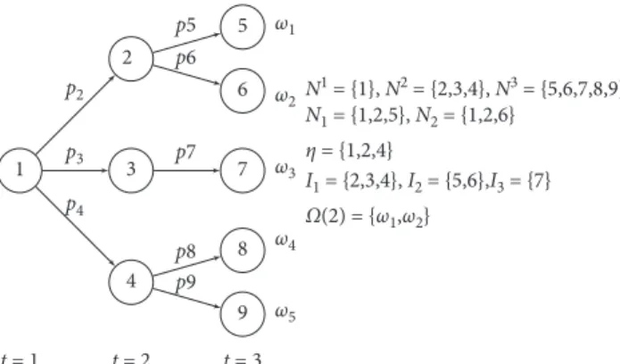
2.1. Scenario Representation. The stochastic program rep-resentation can be visualized as a tree, the so-called “scenario tree.” It can be represented as follows. LetTdenote the set of periods in the planning horizon with T� |T| being the number of periods. In the tree, a node represents the re-alization of the uncertain parameter and variable at a given time period. Let nandN describe the node and the lexi-cographically numbered set of nodes 1{ ,. . .,|N|}in the tree, respectively. From each node n, for t∈T∖{ }T, there is at least one branch leading to another node mwith a condi-tional probabilityp_mwithm∈In, that is, the set of nodes, immediate successors of the node n. 􏽐_m∈I

npm�1. We denote byNt

the subset of nodes belonging to periodtsuch thatN� ∪t∈TNtandNt∩Nt+1�Φfort∈T∖{ }T . LetΩ

represent the finite set of representative scenarios in the tree. A scenarioω∈ Ωis a particular realization of the uncertain parameter represented as a path from the root-node to a leaf-node. Each scenario ω has an associated probability or weight denoted bywω_{. Note that􏽐}

ω∈Ωwω�1. Similarly, let N_ω represent the set of nodes forming the scenario ω. In other words,N_ωis the set of nodes in a path from the root-node to a leaf-root-node. There is a number of scenarios that traverse each node. LetΩ(n)denote the set of scenarios that traverse the node n. We have Ω(1) �Ω, Ω(n)∩ Ω(n′) �

Φ ∀n≠n′ and n, n′∈Nt

. Finally, let S􏽥n denote the set of successor nodes to the noden, forn∈N. We haveN1_{is a}

singleton andS􏽥n�Φforn∈NT

(leaf-nodes). Furthermore, let αn _{denote the immediate ancestor node of node n for} n∈N∖{ }1, sincen�1 is the root-node of scenario tree. To introduce nonanticipativity, we need to defineηas the set of nodes having more than one leaf-node as successor

(|S􏽥n∩NT_|

>1⟹n∈ηA). For instance, in Figure 1, nodes 2 and 3 have as leaf-node successors the set of nodes {5, 6} and {7}, respectively. Therefore, node 2∈ηbut node 3 does not. Finally, LetXωrepresent the matrix of variables for all t∈Tfor the scenario ω∈ Ω. As the result, the stochastic program can be stated as follows:

max X 􏽘 ω∈Ω wωf_ω(X), ₍₁₎ s.t. Xω∈Cω∀ω∈ Ω, (2) Xω�Xω′, ∀ω,ω′∈ Ω(n), ω≠ω′, n∈η. (3)

Equation (1) maximizes the expectation from all sce-narios. Equation (2) says that all the solutions should be feasible with respect to the constraints of the scenario.Cω_is

the feasible set for scenarioω. Finally, equation (3) imposes the nonanticipativity constraints (NACs) which require that the solution up to a periodtfrom two scenarios should be the same if the two scenarios are indistinguishable up to period t. We call this model the extensive form (EF).

Notice that we could write constraint (3) in a different form. LetXω_n: �􏼈xω_1n, xω_2n,. . ., xω_sn􏼉be the vector of variables at noden∈ηunder scenarioω, andxω

snis the state variable of the forest unit or “stand” s. LetZn represent a vector of binary variables at node n. Imposing constraint (4) is equivalent to reinforcing NAC. Progressive hedging exploits the following formulation:

Xω_n − Zn�0, ∀ω∈ Ω(n), n∈η. (4)

2.2. Progressive Hedging. Progressive hedging (PH) is a scenario-based decomposition algorithm proposed by [36] for stochastic programming models. The idea of progressive hedging is to relax the nonanticipativity constraints (NACs, equations (4)) in an augmented Lagrangian manner [18, 22, 35, 36] so that each scenario (subproblem) can be

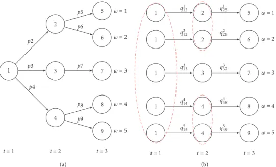
solved independently. This assumes that solving subprob-lems independently is much easier and faster. Non-anticipativity constraints require that values of variables that share the same ancestor nodes should be equal across sce-narios up to that node. In other words, if two scesce-nariosωand ω′are indistinguishable up to periodt, then the solutions of the two scenarios should be the same up to that period. For instance, in Figure 2, each variable at timet�1 should be the same across all the five scenarios and values of variables in period t�2 should be the same for scenarios 1 and 2. However, these constraints are not reinforced when sce-narios are solved independently. Through progressive pe-nalization of violations of NAC, the algorithm is proven to ultimately converge to the optimal solution for convex stochastic programs. In a nutshell, progressive hedging follows the following steps:

(1) Solve each scenario without penalization (2) Compute the average(z)for each variable (3) If solutions have sufficiently converged, then stop (4) Update penalization terms

λ�ρ(x− z) +λ

(5) Solve scenarios with penalization terms (6) Go to step 2

Algorithm 1 describes progressive hedging for multi-stage stochastic programming. The inputs of the algorithm are the penalty factorρ, the maximum number of iterations kmax, and the termination criterionϵ which indicates the level of consensus of nonanticipativity constraints that is acceptable. ε�0 means that the algorithm stops if all the nonanticipativity constraints are satisfied. In the algorithm, line 2 initializes a Lagrangian multiplier(λ)for each NAC constraint. A Lagrangian multiplier is associated with each equation (4). To compute the average, of each variable, we need to have the conditional probability associated to each branch of the scenario tree in the detached form (Figure 2). Equation (5) computes the conditional probability from node n to node mwhich is an immediate successor. That probability (qω

nm) is proportional to the number of leaf-nodes associated with nodembecause the number of leaf-nodes informs on the number of scenarios passing by node m. For instance, from Figure 2,q1

12�q212� (p2/2),q125�p5, andq3

13�p3. Lines 6 and 17 compute the average of each variable at noden∈η. Lines 7 and 18 update the Lagrangian multiplier associated with each nonanticipativity constraint. Line 14 computes the NAC convergence euclidean distance. This distance is zero if all the NACs are satisfied:

qω_nm� pm

|Ω(m)|, ∀m∈In, m∈Nω. (5)

3. Variable Fixation

Progressive hedging variable fixing (PHVF) algorithm is identical to the classic progressive hedging algorithm (Al-gorithm 1). However, instead of letting variables converge progressively, PHVF fixes variables as they converge. Line 10 1 2 3 4 5 6 7 8 9 ω1 ω2 ω3 ω4 ω5 t = 3 t = 2 t = 1 N1 _{= {1}, N}2 _{= {2,3,4}, N}3 _{= {5,6,7,8,9}} N1 = {1,2,5}, N2 = {1,2,6} η = {1,2,4} I1 = {2,3,4}, I2 = {5,6},I3 = {7} Ω(2) = {ω1,ω2} p2 p3 p4 p7 p8 p9 p6 p5

in the progressive hedging algorithm (Algorithm 1) is replaced by Algorithm 2. The algorithm starts by fixing variables in the root-node as they converge. For instance, for a given node n∈η, if a variable has a value of 1 across all scenariosω∈ Ω(n), that variable will be fixed to 1 across all those scenarios. This process is better described in Algo-rithm 2. However, unless a variable belongs to the root-node, it can only be fixed if all variables in the immediate ancestor αn _{have been entirely fixed. The first thing to notice is that}

once the scenario tree is decomposed, there are more sce-narios traversing the root-node (Figure 2). In addition, as we move away from the root-node toward the leaf-nodes, there is a fewer number of scenarios passing by any given node. Hence, if for instance, there are three branches originating from the root-node (as displayed in Figure 2),|I₁| �3, then after fixing the root-node, we get three distinct subextensive forms (SEFs) (Ω(2), Ω(3), and Ω(4)) that can be solved independently (Figure 3). Furthermore, the three SEFs are 1 2 3 4 5 6 7 8 9 ω = 1 ω = 2 ω = 3 ω = 4 ω = 5 t = 3 t = 2 t = 1 p2 p3 p4 p7 p₈ p9 p6 p5 (a) ω = 1 ω = 2 ω = 3 ω = 4 ω = 5 t = 3 t = 2 t = 1 1 2 5 1 2 6 1 3 7 1 4 8 1 4 9 q1 12 q125 q2 12 q226 q3 13 q337 q4 14 q5 15 q549 q4 48 (b)

Figure 2: Example of scenario representation in a compact form (a) and in a detached form (b). The red-dotted ellipses show the

nonanticipativity constraints that need to be imposed.

(1)functionphρ, kmax,ε (2) Initializeλ0,nω�0,∀n∈η,∀ω∈ Ω(n) (3) forω∈ Ωdo (4) x0,ω_{�arg max} x􏼈fω(x):x∈Cω􏼉 (5) end for (6) z0 n�􏽐ω∈Ω(n)qωnmxn0,ω,∀n∈η,∀m∈In (7) λ1,nω�λ 0,ω n +ρ(x0,nω− z0n),∀n∈η,∀ω∈ Ω(n) (8) fork�1 tokmaxdo (9) forω�1 to|Ω|do (10) xk,ω_�argmax x gω(x) �fω(x) − λ k,ω_{(x− z}k− 1_{) − (ρ/2)‖x− z}k−1_‖2 2:x∈Cω 􏼚 􏼛 (11) ϕk ω�maxxgω(x) (12) end for (13) ϕk�􏽐_ω∈Ωwω_ϕk ω (14) if ������������������ 􏽐_ω∈Ωwω_‖xk,ω_{− z}k−1_‖2 2 􏽱 <εthen (15) return(xk_,λk ,ϕk) (16) end if (17) zk n�􏽐ω∈Ω(n)qωnmx k,ω n ,∀n∈η,∀m∈In (18) λkn+1,ω�λ k,ω n +ρ(x k,ω n − z k n),∀n∈η,∀ω∈ Ω(n) (19) end if

(20) return(xkmax_,λkmax_,ϕkmax₎ (21)end function

much easier to solve compared to the original problemΩ(1). The algorithm description exploits that property of the scenario tree.

3.1. Algorithm Description. During PHVF, at each iteration and for each scenario, the problem online 10 of Algorithm 1 needs to be solved. We refer toCω_{as the feasible set created}

by constraint (2) for each scenario. Note that if the un-certainty is only in the objective function (for instance, price uncertainty), then Cω_�Cω′_{,∀ω≠ω′. In this case each}

so-lution of ω is feasible for Cω′_{(ω≠ω′). Since z(·) is the}

average of the values of the variables across scenarios (see line 6 of Algorithm 1), if its value is 1 (or 0), then it means all the scenarios met consensus that the variable should take a value of 1 (or 0), respectively. This realization is exploited in

1 2 3 4 5 6 7 8 9 ω = 1 ω = 2 ω = 3 ω = 4 ω = 5 ω = 1 ω = 2 ω = 3 ω = 4 ω = 5 t = 1 t = 2 t = 3 t = 2 t = 3 2 5 6 3 7 4 8 9 Ω(2) Ω(3) Ω(4)

Figure3: Structure of stochastic problem after fixing the root-node (node 1). The three subextensive forms (SEFs) denoted byΩ(2),Ω(3), andΩ(4)are independent.

(1)functionfixVariablesθ,ω, k

(2) stop�False; (3) fort�1 to|T|do

(4) n:n∈Nt

∩η∩N_ω

(5) ifαn_{is fixed ORnis root-nodethen}

(6) fori�1 to number of standsdo

(7) ifzn,i≥θtthen

(8) FixXω

i,tto 1 (9) else ifzn,i≤1− θtthen

(10) FixXω i,tto 0 (11) else (12) stop�True (13) end if (14) end for (15) end if

(16) ifstop is Truethen

(17) break

(18) else ifnnot marked

(19) Marknas fixed (20) end if (21) end for (22) xk,ω_{�arg max} x gω(x) �fω(x) − λ k,ω_{(x− z}k−1_{) − (ρ/2)‖x− z}k− 1_‖2 2:x∈Cω∗ 􏼚 􏼛

(23) returnfixed nodes (24) end function

Algorithm 2 if it is supposed that the slamming factor θt�1, ∀t. The algorithm moves to the node at the next stage and performs variable fixation if that node belongs to the set of nonanticipativity nodes ηand its predecessor is entirely fixed. The new feasible set created by constraint (2) and fixing some variables is denoted by Cω

∗. Note that this subproblem is much smaller compared to the original subproblem. In Algorithm 2, the inputs are θ, a function defining the value of the slamming factor depending on the staget(0≤θt≤1), see Section 3.3 for more information on this parameter; ωwhich is the scenario; and k which in-dicates the iteration.

Fixing variables impact the optimality since some var-iables may be fixed to values that they may not have taken in the optimal solution. Hence, the algorithm has an impact on the optimality. The objective of fixing variables is not to completely solve the model through the procedure but to obtain a reduced extensive form (REF) that is tractable. Letτ denote the percentage of NAC variables that are fixed before switching to solving the REF.τis a proxy to the number of nodes fixed. The question is what is the appropriateτ that will make the REF tractable while not severely impacting the optimality? The answer to this question is investigated in Section 4.4.1.

3.2. Parallel Implementation. Algorithm 3 is designed for parallel implementation of PHVF. Hence, line 10 from Algorithm 1 has to be replaced by Algorithm 3. At each iteration of progressive hedging, the subproblems can be solved in parallel because they are independent. However, fixing τ variables and switching to solve the reduced ex-tensive form (the exex-tensive form with some variables fixed, REF) is not parallelized. Nonetheless, since our algorithm (PHVF) fixes variables from the root-node to the leaf-nodes, after fixing each node, the problem can be separated into subextensive forms (SEFs) that can be solved independently. For example, as illustrated in Figure 3, after fixing the root-node, we get three separate SEF models. Recursively, each subextensive form model can be solved through variable fixation leading to reduced subextensive form (RSEF). Each RSEF can then be solved directly if its size is deemed tractable. At the end, the solutions from all the REFs can be combined to get the solution of the stochastic program. 3.3. Acceleration Methods. Note from Algorithm 2 that if θt�1, then we fix a variable to 1 (or alternatively to 0) only if all scenarios of interest agree that the value of the variable should be 1 (or 0 alternatively), respectively. This require-ment is hard to meet when dealing with hundreds of sce-narios, especially for the root-node variables which are replicated in all the scenarios. A variable may have the same value in all but one scenario for many iterations. Hence, that scenario slows the convergence. To avoid such a situation, “slamming” [42] forces variables to converge if the per-centage of concordant scenarios for that variable reaches a thresholdθ≤1. However, instead of defining a scalarθas in [42], we definedθt�f(θ0, Q(t))as a function that depends on the stage because if a low value ofθis acceptable for the

root-node, such a value is not acceptable when closer to the leaf-nodes (to avoid infeasibility).θ0is the initial value ofθ, whereasQ(t)can be a linear or exponential function term that increasesθvalue as a function of thet. Notice that if the uncertainty is in the objective function and we apply slamming, then the problem will always be feasible. In our case, preliminary tests allowed us to find the range of ac-ceptable values of θ0. Low values ofθ0 led to infeasibility.

In the same line of thought, even with slamming, there is a chance that the algorithm is locked in a situation where there is no improvement of NAC convergence for many consecutive iterations. We define a “cascading” effect which lowers the value ofθtoθminfor one iteration if the algorithm does not improve (convergence of some nonanticipativity) for αconsecutive iterations. This behavior allows to avoid getting stuck, since lowering θallows to fix some variables for which almost all the scenario already reached consensus. For those variables, the percentage of variables that agree on the value the variable should take is close to θt and the consensus could eventually be reached after several itera-tions. We have noticed that the cascading effect may lead to infeasibility because it may be forcing some variables to a value they would not take otherwise. When infeasibility arises, we roll back and eliminate the cascading effect. In general, there is a tradeoff between infeasibility and the value of θ. Low values of θ lead to a risk of infeasibility while raising that value may make the acceleration methods less efficient.

3.4. Stopping Criteria. In the case of classic progressive hedging, the algorithm stops because we have reached an acceptable level of consensus for NAC or because all the NACs are satisfied. The algorithm terminates as well if the maximum number of iterations (k_max) is reached. In our algorithm, we keep these two stopping criteria, although we know that they may never be reached. We instead rely on the fact that at some points, many nodes will be fixed (NAC consensus is reached for some nodes) and the reduced subextensive forms can be solved directly. The number of NAC consensus reached is checked through the parameterτ which is the percentage of variables fixed. When the per-centage of variables fixed is greater than or equal toτ, the algorithm switches to solve the REF or RSEF.

4. Numerical Experiment

We describe here an empirical performance analysis of our proposed algorithm. For easiness to follow our experiment and replicate the results, we formulate the stochastic version of the so-called “Model I” of forest harvest scheduling.

4.1. Problem Definition and Formulation Indices

ω,ω′: scenario s: stand t: time period

Sets

S: set of stands

Ω: set of scenarios

Ω(n): set of scenarios passing by the noden η: set of nodes on which NAC should be reinforced Nt

: set of nodes at stage t

T: set of time in the planning horizon Parameters

rt: profit from selling wood in periodt($/mbf ). It is the discounted profit that includes selling cost cst: cost of harvesting and hauling wood from stands in periodt($). It is the discounted cost

yω_st: volume of wood harvestable per area from stands in period t according to scenario ω (mbf/ac). This volume depends on the climate that materializes; therefore, it is a parameter that depends on the sce-narioω

as: area of stands(acres)

agest: age of standsat the end of the planning horizon if harvested in yeart

ages·: current age of stands

ages0: age of stand s if not harvested during the planning horizon

f_min: allowable percentage of decrease of volume harvested from one period to another

f_max: allowable percentage of increase of volume harvested from one period to another

wω_{: probability or weight of scenarioω}

Variables

xω_{st: binary variable taking a value of 1 if standsshould}

be harvested in periodtaccording to scenarioω, and 0 otherwise

nω

s: binary variable: 1 if management unitsshould not be harvested during the planning horizon under scenarioω, and 0 otherwise

Hω

t: accounting variable storing the volume of wood harvested in periodtaccording to scenarioω(mbf ):

max􏽘 ω∈Ω wω 􏽘 t∈T r_tHω_t − 􏽘 s∈S c_stxω_st ⎛ ⎝ ⎞⎠ ⎡ ⎢ ⎢ ⎣ ⎤⎥⎥⎦, (6) which is subject to nω_s +􏽘 t∈T xω_st�1, ∀s∈S, ∀ω∈ Ω, ₍₇₎ 􏽘 s∈S asy ω stx ω st�H ω t, ∀t∈T,∀ω∈ Ω, (8) 1− f_min􏼁Hω_t ≥Hω_t+1, ∀ω∈ Ω,∀t�1,. . .,|T| − 1, (9) 1+f_max􏼁Hω_t≤Hω_t+1, ∀ω∈ Ω, ∀t�1,. . .,|T| − 1, (10) 􏽘 s∈S a_s 􏽘 t∈T agestxω_st+ages0nω_s ⎡ ⎣ ⎤⎦_≥􏽘 s asages., ∀ω∈ Ω, (11) xω_st�xω′_st, ∀ω≠ω′;ω,ω′∈ Ω(n);n∈η;t�􏽮t|n∈Nt􏽯; ∀s∈S, (12) xω_st, nω_s �{0,1}, Hω_t ∈R+. (13)

Expression (6) maximizes the profit from timber harvest from all scenarios weighted by their respective probabilities. Constraints (7) require that a stand is at most harvested once during the planning horizon. We use the variable n_s to capture stands that are not prescribed to be harvested during the whole planning horizon. We need that variable to compute the average ending age of the forest as shown in constraints (11). Constraints (8) compute the volume har-vested in each period during the planning horizon. It uses the parameteryω

stwhich values depend on the forest growth scenarioωof interest. Note that the set of constraints (8) is not necessary. We could have written the same model without using that set of constraints. However, doing so would require rewriting constraints (9) and (10), and finally, it would negatively affect the readability of the model. Constraints (9) and (10) impose the even flow constraints so that the volume harvested from one period to another re-main within an allowed fluctuation range. Constraints (11) require that on average, the forest at the end of the planning horizon is at least as old as the forest at the beginning of the planning horizon. Finally, constraints (12) impose the nonanticipativity constraints. It requires that for each stand s, at timet, if two scenarios are indistinguishable, then the decision should be the same for the two scenarios at that time. IfN_ω∩Nω′≠ Φ, then there existstsuch that the two

scenarios are indistinguishable att. Constraints (13) enforce that the decision variables are binary, and the accounting variables are continuous. We remind the reader that vari-ablesHω

t are not required for this model.

4.2. Climate Change Data. The potential mean annual in-crement, which is an indicator of forest growth in a year might change in the Pacific North West because of climate change. The change depends on temperature, precipitation, and air moisture content, all driven by human activities and economic development [28]. In addition, the change is not geographically uniform. Hence, the change tends to be negative in Oregon compared to Washington State. Simi-larly, the change tends to be negative in low altitudes in Oregon. We used the data from [28] which forecast the potential mean annual increment change (pMAI) by the year 2100. The pMAI (m3_{/ha/year) is the potential change in} forest growth that will be observed in a given year; hence, it is a volume given as a function of time and area. We assumed linear change of the growth from now until that year. For

instance, the growth change for next two decades is the double of the growth change for the next decade. The climate paths defined in the Pacific Northwest are A2, A1B, B1, and Commit (or C). Tables 1 and 2 present the values of potential mean annual increment change for each one of the climate paths. In Table 2, climate paths D1 to D4 are artificial climate paths that suppose higher pMAI. We built forest growth scenarios by assuming it is possible to transit from one climate path to another because of mitigation or intensifi-cation of climate change due to human actions.

4.3. Experimental Design. The experiments were conducted under a DELL desktop computer running on Windows with Intel(R) Core(TM) 2 Quad CPU @ 3.70 GHz and 8 GB of memory. During PHVF iterations, each scenario is solved at optimality gap of 1%. This is a premature stop. Nevertheless, this criterion proved to accelerate solution time for each scenario. Furthermore, the last solutions of a mixed integer program are the most difficult ones with no to little im-provement of the objective function value. All the models were solved using IBM ILOG CPLEX 12.6 (CPLEX, [12]). The memory allocated for storing the nodes was 3,000 MB, and the nodes were set to be stored in a compressed format on the hard drive. All other parameters were left to their default values. The code was implemented in Java 10 using Concert Technology of CPLEX.

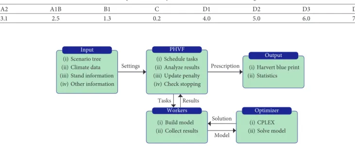
For parallel computation, we used the paradigm of master-workers. The master is in charge of coordinating the PHVF algorithm while distributing the task of solving in-dividual submodels or REF to the workers. Each worker sends back its solution upon completion. The workers compete for access to the memory. Therefore, the choice of the number of workers must be judicious to avoid the overhead which is the amount of time required to coordinate parallel tasks, as opposed to doing useful work. Preliminary experiments showed that two workers was the optimal number given the configurations of the computer. The general framework of the model is presented in Figure 4. The input data contain the information on the forest, the climate change (growth change), and the regulations that ought to be met by the harvest planning. The input is fed to the PHVF

module that is the master governing the optimization process. The workers are the ones interacting with the op-timizer (CPLEX in this case). They send the model to the optimizer which returns the solution. The advantage of this framework is that we could change the optimizer without having to readapt our algorithm. At the end, the output module collects the harvest planning and informs the de-cision making.

Forest growth scenarios were generated using the in-formation on the growth change reported in [28] (see Ta-bles 1 and 2). We assumed that due to climate change and climate change mitigation efforts, it is possible to transition from one climate path to another in two consecutive periods. Hence, for instance, it is possible to transition from climate path A2 in year 2020 to climate path B1 in year 2030. We further assume that the probability of transiting from one climate path to the other is the same. As result, the scenarios are considered equally probable. Note that this assumption does not have much incidence on the performance of the algorithm. Based on the number of scenarios generated, we defined small, medium, and big instances. The small in-stances have 64 scenarios (1×4×4×4×1) which is four branching for the first three periods. The medium instances have 256 scenarios which correspond to four branching for the first four periods (1×4×4×4×4). For small and me-dium instances, pMAI corresponding to each climate path is reported in Table 1. The big instances have 512 scenarios made of eight branching for the first three periods (1×8×8×8×1). The in-depth description of the scenario tree generation methods and its quality are beyond the scope of this research. The interested reader could refer to (1)functionPHVFθ,Ω(j), k

(2) fixed nodes�fixVaribles((θ,ω, k),∀ω∈ Ω(j)) (3) ifproblem small enoughthen

(4) Solve reduced extensive form.

(5) else

(6) fornin fixed nodes which successor are not fixeddo

(7) form∈Indo (8) PHVF(θ,Ω(m), k+1) (9) end for (10) end for (11) end if (12) returnxω (13) end function

ALGORITHM 3: PH variable fixing.

Table 1: Value of pMAI (m3/ha/year) for small and medium

instances. Forests P1 P34 P36 P75 P83 P100 A2 0.5 3.1 −0.3 1.8 0.4 2.1 A1B 0.4 2.5 −0.3 1.6 0.3 1.6 B1 0.4 1.3 0.0 1.0 0.3 1.0 C 0.2 0.2 0.1 0.2 0.1 0.3

[11, 14, 21, 24, 25, 29, 33] and more importantly [34] who describe scenario generation in the forest management framework. We tested our algorithm on six different forests with three being real forests, and the data of which are publicly available1 (P1, P34, P36). The other three were computer-generated forests (P75, P83, P100). The six forests are set to be located in three different altitude classes. The forests are supposed to be located in Oregon and in Washington State. The values of pMAI for the six forests for large instances are reported in Table 2. Table 3 shows the characteristics of the forests and the scenario instances. In the tables, values show the potential mean annual increment change by 2100. Hence, negative values mean there will be a decrease in forest growth, whereas positive values mean that there will be an increase in forest growth.

The medium instances were used as reference to in-vestigate how many variables should be fixed in order to have a problem that is computationally tractable. For that purpose, we solved the stochastic models, using the serial version of our algorithm (Algorithms 1 and 2), settingτto just 20%, 40%, 60%, and 70% before switching to solving the reduced extensive form.τ�20% means some variables are fixed but the root-node is not completely fixed, andτ�40% means that all the root-node variables are completely fixed and some variables from the second period nodes are fixed (as stated before, τ is proxy to the number of nodes fixed. This scheme is possible because there are 25% of NAC variables at each stage and thus at the root-node as well).

We made the experiment by allocating 15, 30, 45, and 60 minutes for each problem. The time is chosen to allow the Table2: Values of pMAI(m3/ha/year)of all the six forests for large instances.

A2 A1B B1 C D1 D2 D3 D4 3.1 2.5 1.3 0.2 4.0 5.0 6.0 7.0 PHVF Workers Input Output Optimizer Settings Prescription Results Tasks Model Solution Scenario tree (i) Climate data (ii) Stand information (iii) Other information (iv) Schedule tasks (i) Analyze results (ii) Update penalty (iii) Check stopping (iv)

Harvert blue print (i) Statistics (ii) CPLEX (i) Solve model (ii) Build model (i) Collect results (ii)

Figure4: Framework of the PHVF algorithm for harvest scheduling under climate change.

Table3: Description of problem size.

Forest |Ω| Binary cols Total cols Rows Nonzeros Stands

P1 64 6,552,015 6,552,335 6,349,760 61,375,488 1,363 256 62,209,423 62,210,703 61,747,968 66,199,808 512 64,286,635 64,289,195 62,798,592 614,320,640 P34 64 612,960 613,280 69,024 633,472 32 256 651,872 653,152 644,288 6,150,272 512 6,100,640 6,103,200 672,704 6,322,560 P36 64 636,045 636,365 623,616 696,576 89 256 6,144,269 6,145,549 6,117,248 6,431,872 512 6,279,905 6,282,465 6,189,440 6,920,576 P75 64 6,121,500 6,121,820 677,632 6,311,808 300 256 6,486,300 6,487,580 6,387,328 61,400,832 512 6,943,500 6,946,060 6,621,568 63,288,576 P83 64 6,121,500 6,121,820 677,632 6,311,104 300 256 6,486,300 6,487,580 6,387,328 61,398,016 512 6,943,500 6,946,060 6,621,568 63,277,312 P100 64 6,121,500 6,121,820 677,632 6,310,400 300 256 6,486,300 6,487,580 6,387,328 61,395,200 512 6,943,500 6,946,060 6,621,568 63,266,048

effect of τ to manifest itself. The tests were run with five repetitions, and the average of the objective function value was reported. Notice that if the time is too long, then eventually all problems can be solved, even the extensive form. Conversely, if the time is too short, then PHVF may not have enough time to finish fixing variables before the time limit and hence low values ofτwill be favored. During the whole experiment, we defined θt�min 0{ .999,

1.05(t−1)_θ

0}. As results, for the first stage (t�1), θ1�θ0. Similarly, we defined θmin�max 0􏼈 .75,θt− 0.05t􏼉. These values were defined from empirical experimentation.

For assessment of our algorithm performance, each problem was solved using our algorithm (PHVF) and comparing that solution to the one obtained by CPLEX solving directly the EF for the equivalent wall clock time. In addition, we report the optimality gap produced by CPLEX

Table4: Effects ofτand allocated time for the forest P1.

Forest ρ Time (min) τ Iterations α θ0 Value Improvement (%)

P1 1000000 15 20 1 6 0.95 371,524,817 — 40 9 6 0.95 386,068,433 3.9 50 18 6 0.95 T NA 60 20 6 0.95 T NA 70 21 6 0.95 T NA 30 20 1 6 0.95 373,450,417 — 40 9 6 0.95 386,156,779 3.4 50 18 6 0.95 385,676,118 3.3 60 20 6 0.95 385,394,686 3.2 70 21 6 0.95 385,258,771 3.2 45 20 1 6 0.95 375,427,413 — 40 9 6 0.95 386,156,779 2.9 50 18 6 0.95 385,676,118 2.7 60 20 6 0.95 385,394,686 2.7 70 21 6 0.95 385,258,771 2.6 60 20 1 6 0.95 375,804,390 — 40 9 6 0.95 386,156,779 2.8 50 18 6 0.95 385,676,118 2.6 60 20 6 0.95 385,394,686 2.6 70 21 6 0.95 385,258,771 2.5

T: termination because PHVF ran out of time while iterating; NA: not applicable;ρ: penalty factor;τ: percentage of variables fixed;α: cascading factor;θ0: initial slamming factor.

Table5: Effects ofτand allocated time for the forest P34.

Forest ρ Time (min) τ Iterations α θ0 Value Improvement (%)

P34 10000 15 20 1 10 0.95 1,333,129 — 40 1 10 0.95 1,332,692 −0.0 50 6 10 0.95 N NA 60 9 10 0.95 N NA 70 18 10 0.95 1,347,152 1.1 30 20 1 10 0.95 1,344,498 — 40 1 10 0.95 1,344,260 −0.0 50 6 10 0.95 N NA 60 9 10 0.95 N NA 70 18 10 0.95 1,347,491 0.2 45 20 1 10 0.95 1,345,620 — 40 1 10 0.95 1,345,761 0.0 50 6 10 0.95 N NA 60 9 10 0.95 N NA 70 18 10 0.95 1,347,555 0.1 60 20 1 10 0.95 1,346,799 — 40 1 10 0.95 1,346,489 −0.0 50 6 10 0.95 1,343,802 −0.2 60 9 10 0.95 N NA 70 18 10 0.95 1,347,759 0.1

N: terminated because could not find feasible solution; NA: not applicable;ρ: penalty factor;τ: percentage of variables fixed;α: cascading factor;θ0: initial slamming factor.

and the gain which is calculated according to gain� (PHVF− EF/EF) where EF is the objective function value obtained by solving directly the extensive form model and PHVF is the solution obtained by PHVF algorithm for the same runtime. For medium and large instances, we report as well the EF value after solving the EF problems for 86,000 seconds (24 hours).

4.4. Results of the Experiment. In addition to the number of scenarios, SMIP size grows as well with the number of units (stands) because we need to define the nonanticipativity constraint for each stand at the time periods on which constraints (12) should be imposed. The problem size in-creases almost by tenfold when going from small instances to the medium ones. The smallest problem in this experiment

Table6: Effects ofτand allocated time for the forest P36.

Forest ρ Time (min) τ Iterations α θ0 Value Improvement (%)

P36 5000 15 20 1 10 0.9 4,468,454 — 40 22 10 0.9 4,513,717 1.0 50 41 10 0.9 4,532,819 1.4 60 51 10 0.9 4,522,013 1.2 70 60 10 0.9 4,525,669 1.3 30 20 1 10 0.9 4,570,040 — 40 22 10 0.9 4,534,327 −0.8 50 41 10 0.9 4,534,156 −0.8 60 51 10 0.9 4,523,000 −1.0 70 60 10 0.9 4,530,669 −0.9 45 20 1 10 0.9 4,616,899 — 40 22 10 0.9 4,534,470 −1.8 50 41 10 0.9 4,534,161 −1.8 60 51 10 0.9 4,532,251 −1.8 70 60 10 0.9 4,530,669 −1.9 60 20 1 10 0.9 4,662,056 – 40 22 10 0.9 4,534,574 −2.7 50 41 10 0.9 4,534,219 −2.7 60 51 10 0.9 4,532,251 −2.8 70 60 10 0.9 4,530,669 −2.8

ρ: penalty factor;τ: percentage of variables fixed;α: cascading factor;θ0: initial slamming factor.

Table7: Effects ofτand allocated time for the forest P75.

Forest ρ Time (min) τ Iterations α θ0 Value Improvement (%)

P75 2000 15 20 1 10 0.9 58,202,734 — 40 19 10 0.9 59,007,403 1.4 50 55 10 0.9 T NA 60 57 10 0.9 T NA 70 70 10 0.9 T NA 30 20 1 10 0.9 58,272,824 — 40 19 10 0.9 59,106,277 1.4 50 55 10 0.9 59,387,884 1.9 60 57 10 0.9 59,324,544 1.8 70 70 10 0.9 59,337,782 1.8 45 20 1 10 0.9 58,297,317 — 40 19 10 0.9 59,131,601 1.4 50 55 10 0.9 59,394,942 1.9 60 57 10 0.9 59,336,592 1.8 70 70 10 0.9 59,354,249 1.8 60 20 1 10 0.9 58,310,384 — 40 19 10 0.9 59,248,444 1.6 50 55 10 0.9 59,395,816 1.9 60 57 10 0.9 59,339,145 1.8 70 70 10 0.9 59,354,525 1.8

T: termination because run out of time iterating; NA: not applicable;ρ: penalty factor;τ: percentage of variables fixed;α: cascading factor;θ0: initial slamming factor.

has 600k + binary variables and over 69k constraints (Table 3).

4.4.1. Impact of τ on the Optimality and Solution Time. Tables 4–9 report the effect ofτon the value of the objective function with respect to the runtime for forests P1, P34, P36, P75, P83, and P100, respectively. We report as well, improvement(%) which is the percentage of increase (if

positive) or decrease (if negative) of the objective function value from the objective function value forτ�20% for the same runtime.

In summary, as expected, everything else being equal, longer runtimes allow a higher objective function. As we can see forτ>40% which corresponds to fixing entirely the root-node and fixing some variables from the second stage, we have numerical issues. The numerical issues have two sources. On one hand, the algorithm may run out of time

Table8: Effects ofτand allocated time for the forest P83.

Forest ρ Time (min) τ Iterations α θ0 Value Improvement (%)

P83 2000 15 20 1 10 0.9 57,970,162 — 40 14 10 0.9 58,558,170 1.0 50 30 10 0.9 58,516,976 0.9 60 32 10 0.9 58,559,069 1.0 70 34 10 0.9 58,592,562 1.1 30 20 1 10 0.9 58,305,853 — 40 14 10 0.9 58,891,381 1.0 50 30 10 0.9 58,833,317 0.9 60 32 10 0.9 58,733,563 0.7 70 34 10 0.9 58,661,347 0.6 45 20 1 10 0.9 59,052,205 — 40 14 10 0.9 58,898,935 −0.3 50 30 10 0.9 58,834,898 −0.4 60 32 10 0.9 58,733,746 −0.5 70 34 10 0.9 58,661,964 −0.7 60 20 1 10 0.9 59,052,215 — 40 14 10 0.9 58,904,481 −0.3 50 30 10 0.9 58,835,134 −0.4 60 32 10 0.9 58,733,734 −0.5 70 34 10 0.9 58,661,851 −0.7

ρ: penalty factor;τ: percentage of variables fixed;α: cascading factor;θ0: initial slamming factor.

Table9: Effects ofτand allocated time for the forest P100.

Forest ρ Time (min) τ Iterations α θ0 Value Improvement (%)

P100 50000 15 20 1 10 0.95 42,331,212 — 40 27 10 0.95 T NA 50 63 10 0.95 T NA 60 69 10 0.95 T NA 70 79 10 0.95 T NA 30 20 1 10 0.95 42,494,130 — 40 27 10 0.95 43,307,744 1.9 50 63 10 0.95 43,298,439 1.9 60 69 10 0.95 N NA 70 79 10 0.95 43,288,841 1.9 45 20 1 10 0.95 42,819,969 — 40 27 10 0.95 43,309,455 1.1 50 63 10 0.95 43,299,189 1.1 60 69 10 0.95 N NA 70 79 10 0.95 43,290,127 1.1 60 20 1 10 0.95 42,931,057 — 40 27 10 0.95 43,309,402 0.9 50 63 10 0.95 43,299,759 0.9 60 69 10 0.95 N NA 70 79 10 0.95 43,290,127 0.8

T: termination because run out of time iterating; N: terminated because could not find feasible solution; NA: not applicable,ρ: penalty factor;τ: percentage of variables fixed;α: cascading factor;θ0: initial slamming factor.

while fixing the variables or finished fixing the variables but does not have enough time to find a feasible solution to the REF. On the other hand, the basis of the REF may be dis-turbed in a way that the number of constraints and variables is not balanced so it is hard for branch and cut algorithm used by CPLEX to find an integral solution for the REF in the allocated time. This is the case for forest P34 with no solution whenτ�60% even when the time is 1 hour. However, for the same forest, there is an integral solution whenτis raised to 70%. This behavior occurred mainly for forest P34 and P100 and is not observed whenτ�40%.

The second aspect is the impact ofτ on the optimality. The advantage that higher values of τ have over the small ones tends to vanish when the runtime is long. Similarly, the improvement in optimality fromτ�40% to higher values of τ is low. In fact, for some forest such as P83, overτ �40%, the objective function value diminishes asτincreases which can be interpreted as during PHVF, many variables are fixed to values that are suboptimal. It clearly appears that fixing just the root-node is the best choice for these problems. It allows sufficient time for REF to find an integral solution while avoiding to impact the optimality, and limiting the disturbance on the structure of the basis matrix.

4.4.2. PHVF versus EF Solved Directly. Table 10 presents the results from PHVF using τ�40% which is equivalent to fixing the root-node and then solving in parallel the SEF. As we can see for the small instances (64 scenarios), solving directly the extensive form outperformed using PHVF. This means the overhead of decomposing the problem into scenarios and solving each one overweighs the benefit. For the medium instances, the results are mixed. Out of the six forests, PHVF outperformed the EF in two cases. Even when

PHVF under performed, it had results that were less than 1% away from the optimal solution. The benefit of using PHVF over the state of art commercial solver such as CPLEX is highlighted when dealing with big instances (512 scenarios). PHVF outperformed the EF for the six forests. In the case of P1 which is the biggest model with 1,363 units (Table 3), EF completely failed to solve the model because it could not fit it in the memory. For other cases for the same runtime, PHVF reached gains ranging from 0.84% to over 767% corre-sponding to forests P34 and P100, respectively. Even after leaving EF for 24 h, PHVF run for 15 min still outperformed in some cases. Comparing the gain to the gap from EF suggests that PHVF almost reached the optimal solution or its solution has a relative optimal gap less than 1%.

5. Conclusions

In this paper, we have developed a method for solving multistage stochastic mixed integer programs that arise in natural resource management such as forest harvest plan-ning. Although tested for growth uncertainty due to climate change, the method is valid as well for other sources of uncertainty such as errors in the model predicting forest growth, and uncertainty in the price of wood. This algorithm is also applicable to other disciplines where the decision variables are binary.

In the forest industry, managers solve multiple instances of the same forest model. It is therefore necessary to have an algorithm that allows one to quickly solve the SMIP. Fur-thermore, having an algorithm that is faster allows the practitioners to explore different management options. However, problems tested in this experiment are quite small compared to the models in the industrial standard. Nev-ertheless, this requirement may be compensated by the

Table10: Comparison of solutions from PHVF and the extensive form.

Same duration with PHVF 24 h

|Ω| Time (s) Forest PHVF EF Gap (%) Gain (%) EF Gap (%) Gain (%)

64 120 P1 2.99E+ 08 3.08E+ 08 0.14 −2.69 — — — 64 120 P34 1.04E+ 06 1.05E+ 06 0.14 −1.64 — — — 64 120 P36 3.48E+ 06 3.73E+ 06 0.32 −6.77 — — — 64 120 P75 4.71E+ 07 4.75E+ 07 1.59 −0.81 — — — 64 120 P83 4.70E+ 07 4.72E+ 07 0.43 −0.46 — — — 64 120 P100 6.53E+ 07 6.54E+ 07 0.51 −0.05 — — —

256 600 P1 3.86E+ 08 3.87E+ 08 0.05 −0.17 3.87E+ 08 0.02 −0.28

256 600 P34 1.35E+ 06 1.33E+ 06 2.38 1.56 1.35E+ 06 0.73 −0.05

256 600 P36 4.73E+ 06 4.64E+ 06 2.05 1.75 4.70E+ 06 0.82 0.52

256 600 P75 5.94E+ 07 5.94E+ 07 0.69 −0.06 5.97E+ 07 0.19 −0.55

256 600 P83 5.90E+ 07 5.93E+ 07 0.28 −0.47 5.93E+ 07 0.22 −0.50

256 600 P100 4.34E+ 07 4.34E+ 07 0.34 −0.06 4.35E+ 07 0.14 −0.22

512 900 P1 2.91E+ 08 NA NA ∞ NA NA ∞

512 900 P34 2.07E+ 06 2.05E+ 06 1.2 0.84 2.07E+ 06 0.27 -0.08

512 900 P36 6.85E+ 06 6.78E+ 06 1.876 1.13 6.79E+ 06 1.64 0.89

512 900 P75 8.48E+ 07 4.50E+ 07 89.57 88.63 8.50E+ 07 0.22 −0.28

512 900 P83 8.47E+ 07 4.49E+ 07 89.44 88.76 8.45E+ 07 0.63 0.27

512 900 P100 4.74E+ 07 5.49E+ 06 767.9 763.3 5.49E+ 06 767.9 763.3

availability of more powerful computation resources in the industry.

The PHVF presented here overcomes some limitations listed in the literature regarding the choice of the penalty termρ. It is documented that large values ofρlead to the phenomenon of cycles [9]. However, because PHVF fixes variables, such a problem is avoided. Notwithstanding all these benefits, PHVF has more parameters that need to be set compared to the classic PH. Fortunately, most of those parameters are easy to set and the limitation remains on the choice of the penalty term ρ. In the preliminary ex-plorations, too low values of ρ led to some numerical issues while too high ones, although accelerated the convergence, negatively impacted the objective function value.

The future extension of this work is to investigate the impact of different parameters on the solution quality. Similarly, having an algorithm that can dynam-ically determine the value of the penalty term would be an improvement for practitioners. On practical aspects, the question of the optimal number of scenarios necessary to approximate the growth change under climate change remains open. This can be done by computing the value of the stochastic solution, the expected value of perfect in-formation for different scenario trees [3, 13, 20, 32].

Appendix

Proof of Infeasibility of Classic Progressive

Hedging Coupled with Variables Fixation

x� x₁₁ x₁₂ x₁₃ x₂₁ x₂₂ x₂₃ x₃₁ x₃₂ x₃₃ x₄₁ x₄₂ x₄₃ ⎡ ⎢ ⎢ ⎢ ⎢ ⎢ ⎢ ⎢ ⎢ ⎢ ⎢ ⎢ ⎢ ⎢ ⎢ ⎢ ⎢ ⎢ ⎢ ⎢ ⎢ ⎢ ⎢ ⎢ ⎢ ⎢ ⎢ ⎢ ⎢ ⎣ ⎤⎥⎥⎥⎥⎥⎥⎥⎥⎥ ⎥⎥⎥⎥⎥⎥⎥⎥ ⎥⎥⎥⎥⎥⎥⎥⎥ ⎥⎥⎥⎦, (A.1)

The variablesxij in the matrixx are all binary.xij �1 means that the standishould be harvested in periodj. Since a stand cannot be harvested more than once,􏽐_jx_ij≤1∀i.

During progressive hedging, at iterationk, we can have this solution. We use the superscript xω _{to refer to the}

solution from scenario ω∈{1,2,3,4}, whenever necessary:

x1� 0 0 1 1 0 0 1 0 0 0 1 0 ⎡ ⎢ ⎢ ⎢ ⎢ ⎢ ⎢ ⎢ ⎢ ⎢ ⎢ ⎢ ⎢ ⎢ ⎢ ⎢ ⎢ ⎢ ⎢ ⎢ ⎢ ⎢ ⎢ ⎢ ⎢ ⎢ ⎢ ⎢ ⎢ ⎣ ⎤⎥⎥⎥⎥⎥⎥⎥⎥⎥ ⎥⎥⎥⎥⎥⎥⎥⎥ ⎥⎥⎥⎥⎥⎥⎥⎥ ⎥⎥⎥⎦, x2� 0 0 1 1 0 0 1 0 0 0 1 0 ⎡ ⎢ ⎢ ⎢ ⎢ ⎢ ⎢ ⎢ ⎢ ⎢ ⎢ ⎢ ⎢ ⎢ ⎢ ⎢ ⎢ ⎢ ⎢ ⎢ ⎢ ⎢ ⎢ ⎢ ⎢ ⎢ ⎢ ⎢ ⎢ ⎣ ⎤⎥⎥⎥⎥⎥⎥⎥⎥⎥ ⎥⎥⎥⎥⎥⎥⎥⎥ ⎥⎥⎥⎥⎥⎥⎥⎥ ⎥⎥⎥⎦ , x3� 0 1 0 1 0 0 0 0 1 0 1 0 ⎡ ⎢ ⎢ ⎢ ⎢ ⎢ ⎢ ⎢ ⎢ ⎢ ⎢ ⎢ ⎢ ⎢ ⎢ ⎢ ⎢ ⎢ ⎢ ⎢ ⎢ ⎢ ⎢ ⎢ ⎢ ⎢ ⎢ ⎢ ⎢ ⎣ ⎤⎥⎥⎥⎥⎥⎥⎥⎥⎥ ⎥⎥⎥⎥⎥⎥⎥⎥ ⎥⎥⎥⎥⎥⎥⎥⎥ ⎥⎥⎥⎦ , x4� 0 1 0 1 0 0 0 0 1 0 1 0 ⎡ ⎢ ⎢ ⎢ ⎢ ⎢ ⎢ ⎢ ⎢ ⎢ ⎢ ⎢ ⎢ ⎢ ⎢ ⎢ ⎢ ⎢ ⎢ ⎢ ⎢ ⎢ ⎢ ⎢ ⎢ ⎢ ⎢ ⎢ ⎢ ⎣ ⎤⎥⎥⎥⎥⎥⎥⎥⎥⎥ ⎥⎥⎥⎥⎥⎥⎥⎥ ⎥⎥⎥⎥⎥⎥⎥⎥ ⎥⎥⎥⎦ . (A.2) 1 2 3 5 6 7 8 ω = 1 ω = 2 ω = 3 ω = 4 t = 3 t = 2 t = 1 (a) ω = 1 ω = 2 ω = 3 ω = 4 t = 3 t = 2 t = 1 1 2 5 1 2 6 1 3 7 1 4 8 (b)

Figure5: Scenario tree of the problem for proof of the PH with direct variable fixation failure when there is uncertainty in the volumes.

Since solutions of the second stage are identical for scenarios 1 and 2, we can fix entirely the variables of the second stage for the two scenarios. Similarly, we can fix entirely the second stage variables for scenarios 3 and 4:

x1_i2�x2_i2� 0 0 0 1 ⎡ ⎢ ⎢ ⎢ ⎢ ⎢ ⎢ ⎢ ⎢ ⎢ ⎢ ⎢ ⎢ ⎢ ⎢ ⎢ ⎢ ⎢ ⎢ ⎢ ⎢ ⎢ ⎢ ⎢ ⎢ ⎢ ⎢ ⎢ ⎢ ⎣ ⎤⎥⎥⎥⎥⎥⎥⎥⎥⎥ ⎥⎥⎥⎥⎥⎥⎥⎥ ⎥⎥⎥⎥⎥⎥⎥⎥ ⎥⎥⎥⎦ , x3_i2�x4_i2� 1 0 0 1 ⎡ ⎢ ⎢ ⎢ ⎢ ⎢ ⎢ ⎢ ⎢ ⎢ ⎢ ⎢ ⎢ ⎢ ⎢ ⎢ ⎢ ⎢ ⎢ ⎢ ⎢ ⎢ ⎢ ⎢ ⎢ ⎢ ⎢ ⎢ ⎢ ⎣ ⎤⎥⎥⎥⎥⎥⎥⎥⎥⎥ ⎥⎥⎥⎥⎥⎥⎥⎥ ⎥⎥⎥⎥⎥⎥⎥⎥ ⎥⎥⎥⎦ , (A.3) xω_i1� 0 1 0 ⎡ ⎢ ⎢ ⎢ ⎢ ⎢ ⎢ ⎢ ⎢ ⎢ ⎢ ⎣ ⎤⎥⎥⎥⎥⎥⎥⎥⎥⎥⎥⎦, ∀ω, i�1,2,4. (A.4)

Comparing variables of the first stage across the four scenarios, we can see that we can fix all variables except for stand 3 which is scheduled for harvest in period 1 for scenarios 1 and 2 but is scheduled for harvest in period 3 for the two other scenarios (equation (A.4)). Therefore, the reduced problem will have all variables fixed except for the third period variables as well asx₃₁for all scenarios. For this problem to be feasible, either x₃₁�0 or x₃₁�1 for all scenarios. However, there is a constraint that links the volume harvested in one period to another (Constraints (9) and (10)). Hence, setting x₃₁�0 means there will be less than acceptable volume in period 1 for scenarios 1 and 2. Similarly, settingx₃₁�1 leads to volume of zero in period 3 for scenarios 3 and 4 which may not be acceptable as well. This situation occurs because the productivity of each stand is different with respect to the scenarios.

Data Availability

The code and the data used in this paper are available upon request or in Github link: https://github.com/MartinBagaram/ proressive-hedging.

Conflicts of Interest

The authors declare no conflicts of interest.

Acknowledgments

Martin B. Bagaram was funded by Precision Forestry Coop of the University of Washington. Andres Weintraub ac-knowledges the support of ANID PIA/Support AFB180003 and Fondecyt 1191531.

References

[1] A. Alonso-Ayuso, L. F. Escudero, M. Guignard, and A. Weintraub, “Risk management for forestry planning under

uncertainty in demand and prices,” European Journal of Operational Research, vol. 267, no. 3, pp. 1051–1074, 2018. [2] E. ´Alvarez-Miranda, J. Garcia-Gonzalo, F. Ulloa-Fierro,

A. Weintraub, and S. Barreiro, “A multicriteria optimization model for sustainable forest management under climate change uncertainty: an application in Portugal,” European Journal of Operational Research, vol. 269, no. 1, pp. 79–98, 2018.

[3] R. M. Apap and I. E. Grossmann, “Models and computational strategies for multistage stochastic programming under en-dogenous and exogenous uncertainties,” Computers & Chemical Engineering, vol. 103, pp. 233–274, 2017.

[4] S. Atakan and S. Sen, “A Progressive Hedging based branch-and-bound algorithm for mixed-integer stochastic programs,” Computational Management Science, vol. 15, no. 6, pp. 501– 540, 2018.

[5] M. B. Bagaram and S. F. T´oth, “Multistage sample average approximation for harvest scheduling under climate uncer-tainty,”Forests, vol. 11, p. 1230, 2020.

[6] J. Barnett, J.-P. Watson, and D. L. Woodruff, “BBPH: using progressive hedging within branch and bound to solve multi-stage stochastic mixed integer programs,” Operations Re-search Letters, vol. 45, no. 1, pp. 34–39, 2017.

[7] J. F. Benders, “Partitioning procedures for solving mixed-variables programming problems,”Numerische Mathematik, vol. 4, no. 1, pp. 238–252, 1962.

[8] P. Beraldi and M. E. Bruni, “A clustering approach for sce-nario tree reduction: an application to a stochastic pro-gramming portfolio optimization problem,” Top, vol. 22, no. 3, pp. 1–16, 2013.

[9] N. Boland, J. Christiansen, B. Dandurand et al., “Combining progressive hedging with a Frank–Wolfe method to compute Lagrangian dual bounds in stochastic mixed-integer pro-gramming,”SIAM Journal on Optimization, vol. 28, no. 2, pp. 1312–1336, 2018.

[10] N. Boland, I. Dumitrescu, G. Froyland, and T. Kalinowski, “Minimum cardinality non-anticipativity constraint sets for multistage stochastic programming,” Mathematical Pro-gramming, vol. 157, no. 1, pp. 69–93, 2016.

[11] M. S. Casey and S. Sen, “The scenario generation algorithm for multistage stochastic linear programming,” Mathematics of Operations Research, vol. 30, no. 3, pp. 615–631, 2005. [12] IBM ILOG CPLEX, “12.6 User’s Manual IBM ILOG CPLEX

Division,”Incline Village, NV, USA, 2019.

[13] N. Di Domenica, G. Mitra, P. Valente, and G. Birbilis, “Stochastic programming and scenario generation within a simulation framework: an information systems perspective,” Decision Support Systems, vol. 42, no. 4, pp. 2197–2218, 2007. [14] J. Dupacov´a, G. Consigli, and S. W. Wallace, “Scenarios for multistage stochastic programs,” Annals of Operations Re-search, vol. 100, pp. 25–53, 2000.

[15] R. Egging, “Benders Decomposition for multi-stage stochastic mixed complementarity problems - applied to a global natural gas market model,”European Journal of Operational Research, vol. 226, no. 2, pp. 341–353, 2013.

[16] L. F. Escudero, M. A. Gar´ın, J. F. Monge, and A. Unzueta, “On preparedness resource allocation planning for natural disaster relief under endogenous uncertainty with time-consistent risk-averse management,”Computers & Operations Research, vol. 98, pp. 84–102, 2018.

[17] M. Fattahi, K. Govindan, and E. Keyvanshokooh, “A multi-stage stochastic program for supply chain network redesign problem with price-dependent uncertain demands,” Com-puters & Operations Research, vol. 100, pp. 314–332, 2018.