Solution methods and bounds for two-stage risk-neutral and multistage risk-averse stochastic mixed-integer programs with applications in energy and manufacturing

2018

Solution methods and bounds for two-stage

risk-neutral and multistage risk-averse stochastic

mixed-integer programs with applications in energy and

manufacturing

Ge Guo

Iowa State University

Follow this and additional works at:https://lib.dr.iastate.edu/etd

Part of theIndustrial Engineering Commons,Operational Research Commons, and theStatistics and Probability Commons

This Dissertation is brought to you for free and open access by the Iowa State University Capstones, Theses and Dissertations at Iowa State University Digital Repository. It has been accepted for inclusion in Graduate Theses and Dissertations by an authorized administrator of Iowa State University Digital Repository. For more information, please [email protected].

Recommended Citation

Guo, Ge, "Solution methods and bounds for two-stage risk-neutral and multistage risk-averse stochastic mixed-integer programs with applications in energy and manufacturing" (2018).Graduate Theses and Dissertations. 16364.

by

Ge Guo

A dissertation submitted to the graduate faculty in partial fulfillment of the requirements for the degree of

DOCTOR OF PHILOSOPHY

Major: Industrial Engineering Program of Study Committee: Sarah M. Ryan, Major Professor

Guiping Hu Lizhi Wang Farzad Sabzikar James D. McCalley

The student author, whose presentation of the scholarship herein was approved by the program of study committee, is solely responsible for the content of this dissertation. The

Graduate College will ensure this dissertation is globally accessible and will not permit alterations after a degree is conferred.

Iowa State University Ames, Iowa

2018

DEDICATION

TABLE OF CONTENTS

DEDICATION ... ii

LIST OF FIGURES ... vi

LIST OF TABLES ... vii

ACKNOWLEDGMENTS ... viii

ABSTRACT ... ix

CHAPTER 1. INTRODUCTION ... 1

1.1 Problem Statement ... 5

1.2 Literature Review ... 7

1.2.1 Solution Algorithms for Stochastic Integer Programs ... 7

1.2.2 Risk-averse Stochastic Programs ... 8

1.2.3 Mixed-Model Assembly Line Sequencing Problems ... 10

1.3 Research Gap... 10

1.4 Outline of Dissertation ... 11

CHAPTER 2. INTEGRATION OF PROGRESSIVE HEDGING AND DUAL DECOMPOSITION IN STOCHASTIC INTEGER PROGRAMS ... 13

Abstract ... 13

2.1 Introduction ... 13

2.2 Scenario Decomposition Algorithms for Stochastic Mixed Integer Programs . 14 2.2.1 Two-Stage Stochastic Mixed-Integer Program ... 15

2.2.2 Dual Decomposition ... 16

2.2.3 Progressive Hedging ... 19

2.3 Integration of PH and DD ... 20

2.3.1 Lower Bounds for PH ... 21

2.3.2 Information Exchange between PH and DD ... 22

2.4 Implementation... 23

2.4.1 DDSIP – Implementation of DD ... 23

2.4.2 PySP – Implementation of PH ... 23

2.4.3 Weight Exchange between PySP and DDSIP ... 24

2.5 Numerical Results ... 26

2.5.1 Server Location ... 26

Acknowledgments ... 31

References ... 31

CHAPTER 3. PROGRESSIVE HEDGING LOWER BOUNDS FOR TIME CONSISTENT RISK-AVERSE MULTISTAGE STOCHASTIC MIXED-INTEGER PROGRAMS... 34

Abstract ... 34

3.1 Introduction: ... 34

3.2 Multistage Stochastic Mixed-Integer Programs ... 36

3.3 Risk Measures ... 38

3.4 Time Consistency of Risk-Averse Multistage Stochastic Programs ... 39

3.4.1 Risk-Averse Multistage Stochastic Programs ... 39

3.4.2 Time Consistency ... 41

3.4.3 Time Consistency for Risk-Averse Multistage Stochastic Programs ... 41

3.5 Scenario Reformulation for Expected Conditional Risk Measures ... 42

3.6 Lower Bounding Approach for Risk-Averse Problems ... 47

3.6.1 Progressive Hedging (PH) Algorithm ... 47

3.6.2 Lower Bounds from PH on Multistage Stochastic Mixed-Integer Programs ... 49

3.6.3 Scenario Bundling in Progressive Hedging ... 50

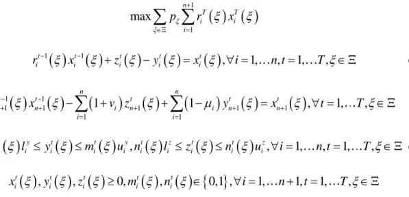
3.6.4 Lower Bounds on E-CVaR Stochastic Mixed-Integer Programs ... 51

3.6.5 Lower Bounds on E-EP Stochastic Mixed-Integer Programs ... 53

3.6.6 Lower Bounds on E-EE Stochastic Mixed-Integer Programs ... 54

3.7 Numerical Results ... 54

3.7.1 Portfolio Optimization Problem ... 55

3.7.2 Lot Sizing Problem ... 59

3.7.3 Generation Expansion Planning Problem ... 61

3.8 Conclusions ... 64

References ... 65

CHAPTER 4. TIME CONSISTENT MULTISTAGE RISK-AVERSE STOCHASTIC MIXED-INTEGER PROGRAMMING APPLIED TO A MIXED-MODEL ASSEMBLY LINE SEQUENCING PROBLEM ... 69

Abstract ... 69

4.1 Introduction ... 69

4.3 Time Consistent Multistage Risk-Averse Stochastic Mixed-Integer

Formulation ... 77

4.3.1 Multistage Risk-Neutral Programs for Model Sequencing Problem ... 77

4.3.2 Time Consistent Multistage Risk-Averse Programs with CVaR Risk Measure ... 80

4.4 Lower Bounding Approach for Time Consistent Risk-Averse Programs... 82

4.4.1 Progressive Hedging Algorithm ... 82

4.4.2 Progressive Hedging Lower Bounds on Stochastic Mixed-Integer Programs ... 84

4.4.3 Lower Bounds on Time Consistent Risk-Averse Programs with CVaR Risk Measure ... 85

4.5 Computational Study ... 87

4.6 Conclusions ... 94

References ... 95

CHAPTER 5. SUMMARY AND DISCUSSION ... 98

LIST OF FIGURES

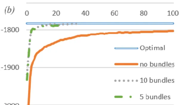
Figure 3.1 Lower bounds from PH and optimal value from solving extensive from for MPO instance with (a) different penalty parameter values; (b) different scenario

bundling strategies with

 

3

10

FX

_ 

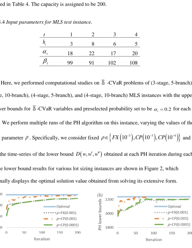
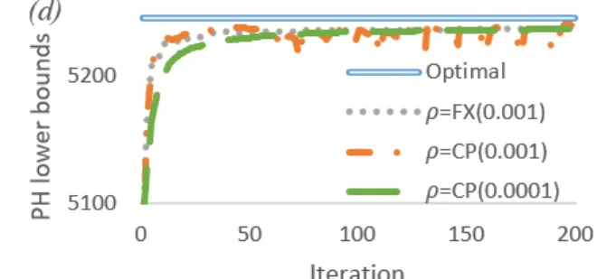
. ... 58 Figure 3.2 Lower bounds from PH and optimal value from solving extensive form for MLS

instances with (a) 3-stage, branch; (b) 3-stage, 10-branch; (c) 4-stage,

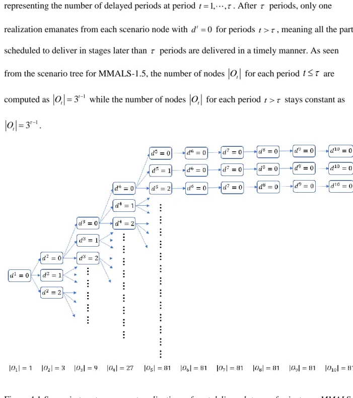
5-branch; (d) 4-stage, 10-branch. ... 61 Figure 4.1 Scenario tree to represent realizations of part delivery lateness for instance

MMALS-1.5. ... 89 Figure 4.2 Lower bounds from PH and optimal value by solving extensive form for

MMALS-2.3 with (a) different penalty parameter values; (b) different scenario

bundling strategies with 3

10



LIST OF TABLES

Table 2.1 DDSIP run-time results on a set of SSLP instances. ... 27

Table 2.2 DDSIP run-time with different ConicBundle parameters for the 5-bus instance. ... 29

Table 2.3 DDSIP run-time with starting multipliers from PH using different



computation strategies for the 5-bus instance. ... 29

Table 2.4 DDSIP run-time and optimality gap on WECC-240 stochastic instance with various starting information. The symbol * denotes failure to converge within 24 hours. ... 31

Table 3.1 Mean values of normal distributions of return rates of assets for MPO test instance. ... 56

Table 3.2 Input parameters for MPO test instance. ... 57

Table 3.3 Computation time for MPO test instance with different scenario bundles. ... 58

Table 3.4 Input parameters for MLS test instance. ... 60

Table 3.5 PH run-time and optimality gap on 8-stage GEP instance with 48-hour time limit. .... 64

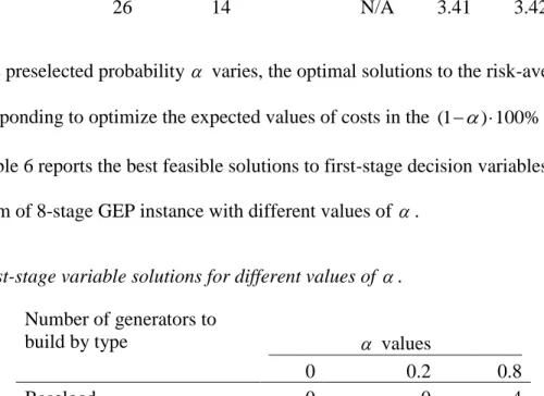
Table 3.6 First-stage variable solutions for different values of . ... 64

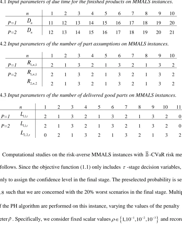
Table 4.1 Input parameters of due time for the finished products on MMALS instances. ... 90

Table 4.2. Input parameters of the number of part assumptions on MMALS instances. ... 90

Table 4.3. Input parameters of the number of delivered good parts on MMALS instances. ... 90

Table 4.4 Lower bounds and time (in seconds) from PH and optimal objective and run-time (in seconds) from EF for a set of MMALS-P. instances. ... 92

ACKNOWLEDGMENTS

I would like to take this opportunity to express my gratitude to those who have helped me throughout my research and the writing of this dissertation and made my five-year Ph.D.

program an unforgettable experience.

I would like to thank my committee chair, Dr. Sarah Ryan, for her constant guidance throughout my Ph.D. study. Her conscientious scholarship and academic integrity has set a role model for me and has inspired me to pursue my career in academia. Her understanding and support in both academic and personal lives has made my years at ISU an enjoyable experience.

I would like to express my very sincere gratitude to my committee members, Dr. Guiping Hu, Dr. Lizhi Wang, Dr. Farzad Sabsikar, Dr. James D. McCalley, and Dr. Mingyi Hong for their great efforts and valuable feedbacks on my research.

I would like to offer my sincere appreciation to my co-authors, Dr. David Woodruff at University of California Davis, Dr. Jean-Paul Watson and Dr. Gabriel Hackebeil at Sandia National Laboratories for their support in the software implementation with Pyomo and their assistance on the computational experiments.

I would also like to thank my colleagues, my instructors, department faculty and staff for making my time at Iowa State University a wonderful experience.

ABSTRACT

This dissertation presents an integrated method for solving stochastic mixed-integer programs, develops a lower bounding approach for multistage risk-averse stochastic mixed-integer programs, and proposes an optimization formulation for mixed-model assembly line sequencing (MMALS) problems.

It is well known that a stochastic mixed-integer program is difficult to solve due to its non-convexity and stochastic factors. The scenario decomposition algorithms display

computational advantage when dealing with a large number of possible realizations of

uncertainties, but each has its own advantages and disadvantages. This dissertation presents a solution method for solving large-scale stochastic mixed-integer programs that integrates two scenario-decomposition algorithms: Progressive Hedging (PH) and Dual Decomposition (DD). In this integrated method, fast progress in early iterations of PH speeds up the convergence of DD to an exact solution.

In many applications, the decision makers are risk-averse and are more concerned with large losses in the worst scenarios than with average performance. The PH algorithm can serve as a time-efficient heuristic for risk-averse stochastic mixed-integer programs with many scenarios, but the scenario reformulation for time consistent multistage risk-averse models does not exist. This dissertation develops a scenario-decomposed version of time consistent multistage risk-averse programs, and proposes a lower bounding approach that can assess the quality of PH solutions and thus identify whether the PH algorithm is able to find near-optimal solutions within a reasonable amount of time.

The existing optimization formulations for MMALS problems do not consider many real-world uncertainty factors such as timely part delivery and material quality. In addition, real-time

sequencing decisions are required to deal with inevitable disruptions. This dissertation formulates a multistage stochastic optimization problem with part availability uncertainty. A risk-averse model is further developed to guarantee customers’ satisfaction regarding on-time performance.

Computational studies show that the integration of PH helps DD to reduce the run-time significantly, and the lower bounding approach can obtain convergent and tight lower bounds to help PH evaluate quality of solutions. The PH algorithm and the lower bounding approach also help the proposed MMALS formulation to make real-time sequencing decisions.

CHAPTER 1. INTRODUCTION

In many applications where decisions are made without full information, stochastic programs are introduced to hedge against consequences of the possible realizations of random parameters so that the expected value of the objective is the best possible. Unlike deterministic programming, stochastic programming describes the uncertain parameters with probability distributions instead of specific values. In two-stage stochastic programs, two categories of decisions are considered. First-stage decisions have to be taken without full information on some random events while recourse actions are taken in response to a particular realization in the second stage. In multistage stochastic programs, the decisions made at each stage can only depend on information revealed before that stage but not after.

Stochastic integer programs are formulated when some of the decisions are required to be integers. For example, unit commitment problems make on and off decisions for thermal electric power generators to minimize the cost of serving unpredictable electricity load; server location problems decide on the optimal server locations to minimize the cost of serving uncertain potential clients; lot sizing problems determine a minimum cost setup, production and inventory schedule to satisfy a stochastic demand over time; and assembly line model sequencing problems yield an optimal production sequence of models subject to unreliable part delivery and quality.

The combination of stochastic parameters and discrete decisions leads to great difficulty in solving stochastic mixed-integer programs. Integer programming is NP-complete. Integer variables make an optimization problem non-convex which is far more difficult to solve than a convex optimization problem is. The solution time grows exponentially in the instance size. When many discrete realizations of the uncertain parameters are possible, a stochastic

mixed-integer program may be formulated as the extensive form of the deterministic equivalent, which is a very large mixed integer program, and therefore even more difficult to solve.

Due to the large scale of extensive forms of stochastic integer programs, decomposition algorithms are widely applied to speed up computation. Generally, the decomposition methods for stochastic integer programs fall into two groups: stage-based methods and scenario-based methods. The exemplary stage-based decomposition method, the L-shaped method, or Benders decomposition [1], is limited to instances with binary variables only in the first stage and easily computable recourse costs. However, the size of the master problem, which is solved for first-stage decisions, keeps increasing as Benders cuts pertaining to later first-stages are added in each iteration. In contrast, scenario-based decomposition methods display advantages in solving the large-scale instances when many realizations are present. Paradigms of scenario-based

decomposition include the Dual Decomposition (DD) algorithm for two-stage stochastic integer programs [2] and the Progressive Hedging (PH) algorithm [3]. The PH algorithm has been proven to converge when all decision variables are continuous and can serve as a heuristic in the mixed-integer case. Computational studies have shown that it can find high-quality solutions within a reasonable number of iterations. To assess the quality of the solutions generated by PH relative to the optimal solution, Gade et al. [4] presented a lower bounding technique for the PH algorithm and showed that for convex problems, the lower bound obtained by PH is as tight as the lower bound from the Lagrangian dual. Furthermore, the PH algorithm can easily extend to multistage formulations with integers in any stage.

Traditional stochastic programming is risk-neutral and optimizes the expected

performance across all scenarios. The optimal solutions to the risk-neutral models perform well in the long run over repeated instances. But for non-repetitive decision-making problems under

uncertainty, the risk-neutral solutions may perform poorly under certain realizations of the uncertain parameters. Therefore, risk-averse models have recently attracted attention in

stochastic programming for decision makers who are more concerned with the large losses in the worst scenarios rather than average performance.

Among a selection of risk measures to include in risk-averse programs, some coherent measures possess suitable mathematical properties to construct efficient algorithms. Two broad categories of coherent risk terms are quantile and deviation based risk measures [5]. Quantile risk-measures are based on the quantiles of the probability distributions of the random objectives. Types of quantile based risk-measures include Excess Probability (EP), which measures the probability of exceeding a prescribed target level; and Conditional Value-at-Risk (CVaR), which

measures the expectation of the



1



% worst outcomes for a given probability. Deviation

risk measures are based on the deviation of the expected value from a prescribed target, and they include Expected Excess (EE), which measures the expected value of the excess over a given target; and Semi-Deviation (SD), which measures the expected value of the excess over the mean.

When risk measures are extended to multiple stages, however, there is no natural way of measuring risk and one key issue of time consistency arises. Generally speaking, re-solving the problem at later stages yields the same optimal objective given the solutions from previous stages if an optimization problem is time consistent. In general, the property of time consistency does not hold for multistage risk-averse models and depends on how the risk measures are computed. Homem-de-Mello and Pagnoncelli [23] proposed a class of expected conditional risk measures (ECRMs) which prove to be time consistent and, for some risk measures, allow for risk-neutral reformulations. The scenario-decomposed reformulations with various risk measures

allow for the employment of scenario decomposition solution algorithms, such as the PH algorithm, to efficiently solve multistage risk-averse problems. However, approaches to assess PH solution quality for risk-averse models have not been explored. An approach to obtain lower bounds from the PH algorithm, if found, not only can evaluate the PH solution quality, but also can integrate the PH algorithm with exact algorithms that rely on lower bounds such as the DD algorithm for two-stage problems. Most importantly, the lower bounding approach can help the PH algorithm to find near-optimal solutions within a reasonable amount of computational time. A novel application of multistage stochastic mixed-integer programs arises in shop floor control. Mixed-model assembly line manufacturing systems have become popular in recent years as an important part of the just-in-time production system, in which several models of the same basic product are manufactured on the same production line. The optimal design and operation of mixed-model assembly lines must address a long-term assembly line balancing problem to assign tasks to stations and a short-term model sequencing problem to determine the production

sequence of a given set of models within the planning horizon.

A number of optimization models have been proposed for the model sequencing problem in mixed-model assembly line manufacturing system. Some formulations also considered

uncertainty factors such as demand from customers and operation times. In the real world, however, mixed-model assembly lines are faced with more challenging uncertainties including timely part delivery, material quality, upstream sub-assembly completion and availability of other resources. In addition, assembly lines must meet deadlines imposed by customers or downstream stations. All those uncertainties play an important role in making sequencing decisions, but are not yet addressed in existing formulations.

In just-in-time manufacturing systems such as mixed-model assembly lines, the schedulers are most concerned with the on-time performance in worst scenarios rather than average performance when large losses are resulted from unreliable part availability. There are two open issues in this context. First, the objective of on-time performance has not been explored in existing optimization models. Second, risk-neutral models yield the optimal performance across all the scenarios while the optimization of performance in worst scenarios requires risk-averse models, which have not been explored either.

The formulation of optimization models to make sequencing decisions was motivated by a project aimed at developing a shop floor decision support system in collaboration with

industrial partners. The optimization model could serve as a decision-support tool in the

sequencing module of this system. Real-time resequencing decisions are required in this project to avoid wastage in time and costs of downtime caused by inevitable disruptions. Therefore, a time efficient solution algorithm is desired to find near-optimal solutions within a reasonable amount of time.

1.1 Problem Statement

This dissertation addresses the following interrelated questions.

First, the PH algorithm and the DD algorithm are two paradigms of scenario-based decomposition solution algorithms for two-stage stochastic programs and have both displayed computational advantages for solving stochastic mixed-integer programs with a large number of scenarios. However, both of these two solution algorithms have their own deficiencies. Although the PH algorithm can find high-quality solutions within a reasonable number of iterations, the solutions are not guaranteed to converge to global optimality in the case of mixed-integer problems. The DD algorithm, on the other hand, can achieve global convergence but the branch and bound process may be slow. Therefore, a question is brought up: can we combine the

advantages of the PH and DD algorithms by proposing an integrated approach? Given the PH lower bounding approach presented by Gade et a. [4] and the fact that for convex problems, the lower bound from PH is as tight as the lower bound from the Lagrangian dual, we are seeking a way to exchange the information of solutions and objectives between the PH algorithm and the DD algorithm through their lower bounds.

Second, the classical formulation of stochastic programs assumes that the decision maker is risk-neutral such that he or she will not mind large losses in some scenarios as long as those are offset by large gains in other scenarios. This formulation, however, does not reflect the situation where the decision maker is more concerned about large losses, that is, the decision maker is risk-averse. It is natural to consider risk-averse formulations of stochastic programs. Time consistency is an important issue in modeling multistage risk-averse models. In general, time consistency for multistage risk-averse stochastic programs is not guaranteed. Therefore, we are seeking a time consistent scenario-decomposed version of reformulations for multistage risk-averse models that allow for the application of scenario decomposition solution algorithms such as the PH algorithm. Essentially, we want to propose a lower bounding approach from the PH algorithm for multistage risk-averse programs to assess the PH solution quality and thus identify whether the PH algorithm is able to find near-optimal solutions within a reasonable amount of computational time.

Third, as the most important short-term problem in mixed-model assembly line

manufacturing system, the model sequencing problem has been studied extensively as seen in a variety of optimization formulations to determine the optimal production sequence. However, the existing formulations are incomplete and do not model many real-world uncertainties such as timely part delivery and material quality. To incorporate those uncertainties in our

decision-making process, we would like to propose an optimization model with part availability modeled as a stochastic process. In addition, in just-in-time manufacturing systems such as mixed-model assembly lines, the schedulers tend to worry more about the on-time performance in worst scenarios. For such decision makers concerned with large losses in worst scenarios, a risk-averse model is preferred. The critical question is, which risk measure should be selected to represent the on-time performance in worst scenarios? Furthermore, can this risk-averse model provide us with near-optimal sequencing decisions in real time to decrease the downtime of assembly lines?

1.2 Literature Review 1.2.1 Solution Algorithms for Stochastic Integer Programs

The presence of discrete decision variables leads to great difficulty in solving stochastic integer programs due to the NP-hard nature of integer programming. Until now much progress has been made in developing algorithms, extending from special instances to more general stochastic mixed-integer programs. Stage-based decomposition algorithms were studied for various classes of two-stage stochastic integer programs. Laporte and Louveaux [1] proposed integer L-shaped methods for stochastic integer programs so long as the first-stage decisions are binary. Sen and Sherali [6] presented branch-and-cut approaches for two-stage stochastic integer programs. Ahmed [7] introduced a branch-and-bound algorithm for two-stage stochastic integer programs. As for multi-stage stochastic integer programs, several scenario decomposition methods were proposed. Lulli and Sen [8] presented a branch-and-price (B&P) algorithm for multi-stage stochastic integer programs. Carøe and Schultz [2] developed a dual decomposition (DD) algorithm based on scenario decomposition and Lagrangian relaxation. Lubin et al. [9] demonstrated the potential for parallel speedup by addressing the bottleneck of parallelizing dual decomposition. Originally proposed by Rockafellar and Wets [3] for stochastic programs with only continuous variables, progressive hedging (PH) has been successfully applied by Listes and

Dekker [10], Fan and Liu [11], Watson and Woodruff [12], and many others as a heuristic to solve stochastic mixed-integer programs. To assess the quality of the solutions generated by PH relative to the optimal solution, Gade et al. [4] presented a lower bounding technique for the PH algorithm and showed that for convex two-stage problems, the lower bound obtained by PH is as tight as the lower bound obtained from the Lagrangian dual.

1.2.2 Risk-averse Stochastic Programs

Extensive studies have been performed in the formulation and solution algorithms for two-stage risk-averse models. Schultz and Tiedemann [13] presented a mixed-integer linear programming formulation of a mean-risk model involving CVaR as risk measure in the framework of two-stage stochastic mixed-integer programming. Fábián [14] proposed

decomposition frameworks for handing CVaR objectives and constraints in two-stage stochastic models. Miller and Ruszczynski [15] developed a nested formulation of a risk-averse two-stage program and presented a risk-averse multicut decomposition method. Noyan [16] developed decomposition algorithms for a risk-averse two-stage stochastic programming model with CVaR as the risk measure. Venkatachalam and Ntaimo [17] presented a stage-wise decomposition method for stochastic programs with binary variables in the second-stage with absolute semi-deviation risk measure.

For multi-stage stochastic programs, however, there is no obvious way of measuring risk. The difficulty in extending risk measures to the multistage setting has been discussed in several papers. Some papers discuss how to adapt existing algorithms from the risk-neutral case to the risk-averse case, often with the CVaR as the risk measure. Collado and Papp [18] introduced a partial bundle method for risk-averse multistage stochastic optimization. Eichhorn and Römisch [19] defined a class of polyhedral risk measures with favorable properties and proposed

programs. Guigues and Sagastizábal [20] proposed a risk-averse rolling-horizon time consistent approach and showed the risk-averse formulations of stochastic linear programs are numerically tractable. Kozmik and Morton [21] proposed a new approach of upper bound estimator for minimization problems in risk-averse multi-stage stochastic programs using CVaR as risk measure. Pflug and Pichler [22] proposed a time consistent formulation of multi-stage stochastic program with CVaR and presented a stage-wise dynamic decomposition.

It has been observed that one very important issue in modeling risk-averse multi-stage stochastic programs is that of time consistency. It is a desirable property for multi-stage stochastic programs. Shapiro [23] defines a problem to be time consistent if the solution at a node in the scenario tree does not depend on children of other nodes. Carpentier et al. [24] formulated the property of time consistency such that the optimal strategies obtained when solving the original problem remain optimal for all subsequent-stage problems. Pflug and Pichler [25] claim a multistage stochastic program to be time consistent if, when resolving the problem at later stages, the original solutions remain optimal for those stages. Homem-de-Mello and Pagnoncelli [26, p.189] define time consistency informally as “if you solve a multi-stage stochastic program and find solutions today, you should find the same solutions if you re-solve the problem tomorrow given what was observed and decided today”.

Given that the property of time consistency is not guaranteed for multistage risk-averse models, significant efforts are initiated to find time consistent risk measures for multistage stochastic programs. Ruszczynski and Shapiro [27] proposed a nested conditional risk measure for multistage optimization problems which proves to be time consistent. The nested conditional risk measure is formulated in a recursive function which is not given in explicit form. Homem-de-Mello and Pagnoncelli [26] addressed this drawback by proposing a class of expected

conditional risk measures which prove to be time consistent and can lead to a risk-neutral reformulation.

1.2.3 Mixed-Model Assembly Line Sequencing Problems

Modeling of sequencing problems has been studied in recent papers with the development of mixed-model assembly line manufacturing systems. Rahimi-Vahed [28] considered three objectives to be minimized in a mixed-model assembly line sequencing problem: total utility work, total production rate variation, and total setup cost. Rabbani et al. [29] developed a bi-objective optimization model to find the optimal sequence of products to minimize the total cost as well as to maximize levels of customer satisfaction. In addition, some studies are performed on the optimization modeling with a variety of uncertainties. Boysen [30] discussed three major sequencing approaches including mixed-model sequencing, car sequencing and level scheduling considering two major uncertainties of stochastic demand and task times. Zhao [31] formulated an optimization problem of daily scheduling to minimize the expected system cost including the inventory cost of holding products and the penalty cost of backorders with stochastic demand. Dong [32] proposed a stochastic programming formulation to minimize the expected work overload time for a mixed-model assembly U-lines with stochastic task times. As the problem is NP-hard, a simulated annealing algorithm is proposed to solve this problem.

1.3 Research Gap

Based on the current literature review, the existing gaps studied in this research are as follows:

(1) Given the advantages of two scenario decomposition solutions algorithms, there did not exist an approach to combine the computational efficiency of the PH algorithm and the global optimality of the DD algorithm. Now that the lower bound from PH is as tight as the lower bound from the Lagrangian dual for convex problems, it is yet unrevealed how the

information can be exchanged between the PH algorithm and the DD algorithm through their lower bounds. This gap has been filled in our research work [33].

(2) It is natural to consider risk-averse models for decision makers who are more concerned with large losses in worst scenarios. For multistage risk-averse models, the property of time consistency is desired. There did not exist scenario reformulations for time consistent multistage risk-averse stochastic programs to allow for the application of scenario decomposition solution algorithms such as the PH algorithm. Furthermore, a lower bounding approach is not available for multistage risk-averse models to help the PH algorithm to find near-optimal

solutions within a reasonable amount of time. This gap has been filled in our research work [34]. (3) The existing formulations for model sequencing problems in mixed-model assembly line manufacturing systems are incomplete and do not model some important real-world

uncertainties such as timely part delivery and material quality. In addition, the schedulers tend to be more concerned with on-time performance in worst scenarios. Thus, a risk-averse model with part availability uncertainty is to be proposed to find optimal sequencing decisions. Besides, a time efficient solution algorithm is to be identified to find near-optimal solutions in real time for a just-in-time manufacturing system. This gap has been filled in our research work [35].

1.4 Outline of Dissertation

Chapter 2 presents a method for integrating PH and DD algorithm for solving stochastic integer programs based on the correspondence between lower bounds obtained with PH and DD algorithm [33]. In chapter 3, we propose a scenario-decomposed version of risk-neutral

reformulation for time consistent multistage risk-averse models, and present an approach to obtain convergent and tight lower bounds from the PH algorithm for time consistent multistage risk-averse models [34]. A multistage stochastic model for mixed-model assembly line

availability uncertainty. The lower bounding approach from [34] is applied to its risk-averse version as the solution algorithm in the context of real-time resequencing [35]. Chapter 5 concludes this dissertation with its contributions, limitations, and future studies.

CHAPTER 2. INTEGRATION OF PROGRESSIVE HEDGING AND DUAL DECOMPOSITION IN STOCHASTIC INTEGER PROGRAMS

A paper published in Operations Research Letters

Abstract

We present a method for integrating the Progressive Hedging (PH) algorithm and the Dual Decomposition (DD) algorithm of Carøe and Schultz for stochastic mixed-integer programs. Based on the correspondence between lower bounds obtained with PH and DD, a method to transform weights from PH to Lagrange multipliers in DD is found. Fast progress in early iterations of PH speeds up convergence of DD to an exact solution. We report

computational results on server location and unit commitment instances.

Keywords: Stochastic programming; Mixed-integer programming; Progressive hedging;

Dual decomposition; Lower bounding

2.1 Introduction

Stochastic mixed-integer programs find a broad application in energy, facility location, production scheduling and other areas where a set of decisions must be taken before full information is revealed on some random events and some of the decisions are required to be integer [1]. The combination of uncertainty and discrete decisions leads to the difficulty in solving stochastic mixed-integer programs.

Until now much progress has been made in developing algorithms to solve these

problems, extending from special instances [12, 13, 23] to more general stochastic mixed-integer programs [2, 20]. Carøe and Schultz [3] developed a dual decomposition (DD) algorithm based on scenario decomposition and Lagrangian relaxation. Lubin et al. [14] demonstrated the potential for parallel speedup by addressing the bottleneck of parallelizing dual decomposition. Originally proposed by Rockafellar and Wets [19] for stochastic programs with only continuous

variables, progressive hedging (PH) has been successfully applied by Listes and Dekker [17], Fan and Liu [6], Watson and Woodruff [25], and many others as a heuristic to solve stochastic mixed-integer programs. To assess the quality of the solutions generated by PH relative to the optimal solution, Gade et al. [8] presented a lower bounding technique for the PH algorithm and showed that the best possible lower bound obtained from PH is as tight as the lower bound obtained using DD.

The PH algorithm can find high-quality solutions within a reasonable number of iterations, but is not guaranteed to converge to a globally optimal solution in the case of mixed-integer problems. The DD algorithm, on the other hand, will achieve convergence combined with branch and bound but may be slow. This paper combines advantages of both scenario

decomposition methods. By transforming PH weights into Lagrangian multipliers as a starting point for DD, the convergence of DD can be sped up considerably.

The remainder of this paper is organized as follows. In Section 2 we describe the PH and DD algorithms, two scenario-based decomposition algorithms for stochastic mixed-integer programs. Our integration approach to transfer information from PH to DD is developed in Section 3. In Section 4, we document the implementation of our integration method and in Section 5, provide experimental results on a set of stochastic server location instances and two stochastic unit commitment instances.

2.2 Scenario Decomposition Algorithms for Stochastic Mixed Integer Programs

Decomposition methods for stochastic programs generally fall into two groups: stage-based methods and scenario-stage-based methods [18]. The exemplary stage-stage-based decomposition method is the L-shaped method, or Benders decomposition [21]. Paradigms of scenario-based decomposition include the PH algorithm [19] and the DD algorithm [3]. One advantage of scenario-based decomposition methods over the stage-based ones is their mitigation of the

computational difficulty associated with large problem instances by decomposing the problem by scenario and solving the subproblems in parallel. In practical applications, PH can easily be implemented as a “wrapper” for existing software for large-scale implementation of the deterministic scenario problems. In this section, we will discuss these two scenario-based decomposition methods for stochastic mixed-integer programs in detail.

2.2.1 Two-Stage Stochastic Mixed-Integer Program

We consider the following two-stage stochastic mixed-integer program:





min ( ) : ,

z cx Q x Axb xX , (1)

where Q x( ) 

 

( , )x and  ( , )x min



q( ) : y Wyh( ) T( ) , x y Y



. Here

1

n T

c  and _b m1 _{are known vectors, while A} m n11 _{and W} m2n2 _{are known matrices.}

The vector  is a random variable defined on some probability space ( , , )  P and for each

, the vectors

q

( )



T



n2 _and

h

( )





m2 _{and the matrix T( )}  m2n1_{. The sets X} n1





and _Y n2



 denote the mixed-integer requirements on the first-stage and second-stage

variables. The decisions are two-stage in the sense that first-stage decisions x have to be taken

without full information on some random events while second-stage decisions

y

are taken after

full information is received on the realization of the random vector . The notation _denotes

expectation with respect to the distribution of .

To avoid complications when computing the integral behind _ we assume that we have

only a finite number of realizations of , known as scenarios



j, j1,...,r, with corresponding

linear program with a block-angular structure called the extensive form of the deterministic equivalent: 1 min : ( , ) , 1,..., r j j j j j j z cx p q y x y S j r     _    _ 



, (2) where Sj 



( ,x yj) :Axb x, X Wy, j hjT x yj , jY



.

The block-angular structure of Eq. (2) enables the decomposition methods to split it into scenario subproblems by introducing copies of the first-stage variables. This idea leads to the so-called scenario formulation of the stochastic program:

1 1 min ( ) : ( , ) , 1,..., , ... . r j j j j j j j r j z p cx q y x y S j r x x     _      _ 



 (3)

The subproblems are coupled by the non-anticipativity constraints, 1

... r

x  x , which

force the first-stage decisions to be scenario-independent.

2.2.2 Dual Decomposition

The dual decomposition (DD) algorithm of Carøe and Schultz relaxes the

non-anticipativity constraints and uses branch and bound to restore non-non-anticipativity. DD obtains lower bounds on the optimal value of problem (3) by solving the Lagrangian dual obtained by relaxing the non-anticipativity constraints.

The non-anticipativity requirement of problem (3) can be expressed by several equivalent representations. Lulli and Sen [15] as well as Lubin and Martin [14] introduce an additional

variable x. and model non-anticipativity as

. 0, 1,... j

x  x j r, (4)

while Carøe and Schultz represent non-anticipativity by

1 0, r j j j H x  



(5)

where the matrix _Hj n r1(  1) n1_.

Using anticipativity representation (4), the Lagrangian relaxation of non-anticipativity constraints may be written as

1 ( ) min [ ( , , ) .] : ( , ) , r j j j j j j j j j P  R x y   x x y S     _   _ 



 (6)

where R x y_j( j, j,j) p cxj( jq yj j)jxj for j1,...,r and the parameter

1

(



j T

)



n . The Lagrangian (6) is separable into 1

1 ( ,..., ) ( ), r r j j j P   P   



where





( j) min ( j, j, j) : ( j, j) j j j P   R x y  x y S , (7)

with the condition

1 0 r j j   



required for boundedness of the Lagrangian. The

Lagrangian dual is expressed as

1 1 ,..., 1 max r ( ,..., ) : 0 . r r j LD j c _{ } P        _  _ 



 (8)

The non-anticipativity representation (5), on the other hand, leads to the Lagrangian relaxation in the form

1 ( ) min ( , , ) : ( , ) , r j j j j j j j D  L x y  x y S     _  _ 



 (9)

where L x y_j( j, j, )  p cxj( jq yj j)(H xj j) for j1,...,r, where the vector

1 1

( ,...,

r

)

 







and the vector

(



j T

)



n1

. The Lagrangian (9) is separable into

1 ( ) ( ), r j j D  D   



where





( ) min ( j, j, ) : ( j, j) j . j j D   L x y  x y S (10)

The Lagrangian dual problem then becomes the problem

max

( ).

LD

z



_

D



(11)

The Lagrangian dual (11) is a convex non-smooth program and can be solved using subgradient methods.

Due to the integer requirements in Eq. (2), a duality gap may occur between the optimal value of the Lagrangian dual (11) and the optimal value of Eq. (2) as described in the proof of Proposition 2 in [3]. The Lagrangian dual (11) provides lower bounds on the optimal value of Eq. (2) and the optimal solutions of the Lagrangian relaxation. In general, these first-stage solutions will not coincide unless the duality gap vanishes. The DD algorithm employs a branch and bound procedure that uses Lagrangian relaxation of non-anticipativity constraints as lower bounds [3].

STEP 1 Initialization: Set z*   and let

P

consist of problem (2). STEP 2 Termination: If

P

  and z* , then *

x with

z

*



cx

*



Q x

( )

* is optimal. STEP 3 Node selection: Select and delete a problem

P

from

P

, solve its Lagrangian

dual (11). If the associated optimal value

z

_LD

( )

P

equals infinity go to STEP 2.

STEP 4 Bounding: If

z

_LD

( )

P

is greater than z* go to STEP 2. Otherwise proceed as

follows; if the first-stage solutions

x j

j

,



1,..., ,

r

of the subproblems are

(1) identical, then set _z*_{: min}



_{z cx}*_, j_{Q x(} j₎



_.

(2) not identical, then compute a suggestion

x

ˆ



Heu x

( ,..., )

1

x

r using some heuristic. If

x

ˆ

STEP 5 Branching: Select a component x_{( )k} of xˆ and add two new problems to that differ from

P

by the additional constraint x_{( )k}   xˆ_{( )k}  and x_{( )k} _xˆ_{( )k} _1, respectively, if x( )k is

integer, or x_{( )k}  xˆ_{( )k} 



and x_{( )k} xˆ_{( )k} 



, respectively, if x_{( )k} is continuous. The value of

0



 must be chosen such that the two new problems have disjoint subdomains. Go to STEP 3.

2.2.3 Progressive Hedging

Proposed by Rockafellar and Wets [19], the progressive hedging (PH) algorithm is a scenario decomposition method for stochastic programs motivated by augmented Lagrangian theory. By decomposing the extensive form into scenario subproblems, the PH algorithm effectively reduces the computational burden of solving extensive forms directly, especially for large-scale problem. Solving scenario subproblems separately can also take advantage of any special structures that are present.

A scenario solution is said to be admissible if it is feasible in one scenario; a scenario solution is said to be implementable or non-anticipative if its first-stage decision is scenario-independent; a solution is feasible if it is both admissible and implementable. The idea of the PH algorithm is to aggregate the admissible solutions of modified scenario subproblems, which progressively causes the aggregated solution to be non-anticipative and optimal. The modified scenario subproblem comes from scenario decomposition of the augmented Lagrangian as a close approximation of problem (3). The modified cost function includes a penalty term relative to the non-anticipativity constraint and a proximal term that measures the deviation of the scenario solution from the aggregated solution for first-stage decisions. The weight vector

1

n s

w  is updated by the penalty parameter (vector)  0 in each iteration. This weight

update rule is essential to the proofs of the convergence theorems [19].

The PH algorithm has been proven to converge when all decision variables are

continuous and can serve as a heuristic in the mixed-integer case. The basic PH algorithm for two-stage stochastic mixed-integer programs proceeds as follows [8]:

STEP 1 Initialization: Let v: 0 and w_vj: 0 , j1,...,r. For each j1,...,r , compute





1 1 , ( , ) : arg min j j : ( , ) j j j j j j j j v v x y x_ y_  cx q y x y S

STEP 2 Iteration update: v v 1

STEP 3 Non-anticipative policy:

1 : r j j v _v j x p x  



STEP 4 Weight update: w_vj:w_vj_1(x_vj xv),j1,...,r

STEP 5 Decomposition: For each j1,...,r , compute

2 1 1 _, ( , ) : arg min : ( , ) 2 j j j j j j j j j j j v v v _{x y} v x_ y _  cx q y w x



x x x y S   

STEP 6 Termination: If all the first-stage scenario solutions 1

j v

x _ agree, then stop.

Otherwise, return to Step 2.

While convergence is not guaranteed for mixed-integer problems, computational studies have shown that the PH algorithm can find high-quality solutions within a reasonable number of iterations [25]. The PH algorithm also applies to multi-stage stochastic programs with discrete variables in any stage.

2.3 Integration of PH and DD

In view of the fact that the PH algorithm can find high-quality solutions within a

reasonable number of iterations but is not guaranteed to converge in the mixed-integer case and the DD algorithm is exact but may be slow, fast progress in early iterations of PH could speed up convergence of DD to an exact solution if the PH algorithm can be combined with the DD

algorithm. We now demonstrate how PH and DD can be integrated through their lower bounds. We first review the lower bounding technique for the PH algorithm proposed by Gade et al. [8] and recall equivalence between the best lower bounds obtained by the PH algorithm and the Lagrangian dual from the DD algorithm. Finally, we establish relationships between PH weights and DD multipliers.

2.3.1 Lower Bounds for PH

Although the PH algorithm has been successfully applied as a heuristic to solve multi-stage stochastic mixed-integer programs, it is limited by the lack of convergence guarantee as well as the lack of information to evaluate solution quality relative to the optimal objective. Gade et al. [8] corrected this deficiency of the PH algorithm by presenting a method to compute lower bounds in PH for two-stage and multi-stage stochastic mixed-integer programs. This not only allows us to assess the quality of the solutions in each iteration, but also can provide lower bounds for solution methods, such as branch-and-bound, that rely on them. We restate

Proposition 1 of [8], which shows that the weights w define implicit lower bounds, D w( ), on

the optimal objective value of denoted by z.

Proposition 1 [8]. Let

w j

j

,



1,... ,

r

satisfy

1 0 r j j j p w  



. Let





( j) : min j( j j j j j) : ( j, j) j j D w  p cx q y w x x y S . (12) Then 1 ( ) : ( ) . r j j j D w D w z  



 It can be verified 1 0 r j j j p w  



is maintained in every iteration by the weight update rule.

Proposition 1 indicates that one can compute a lower bound on z in any iteration of the PH

2.3.2 Information Exchange between PH and DD

Theorem 5.1. of Rockafellar and Wets [19] states that, in the convex case, the sequence 1

1

ˆ

{( ,xv



 wv)}_v_ from PH converges to a pair

( ,

x

*



1

w

*

)

such that *

x solves the primal problem

and *

w solves the dual problem. In the mixed-integer case, however, a duality gap may occur

because of the introduced nonconvexity. We restate Proposition 2 in [3], which follows from Theorem II.3.6.2 in [27], to provide insight into why this duality gap arises.

Proposition 2. The optimal value

z

_LD of the Lagrangian dual (11) equals the optimal

value of the linear program

min pj(cxj+qjyj) j=1 r

å

: (xj,yj)Îconv Sj,j=1,...,r,x1=...=xr ì í îï ü ý þï, (13)

where conv denotes convex hull.

Gade et al. [8] show that by applying the PH algorithm to the linear program (13), one can recover both primal and dual optimal solutions to (13) and (11), respectively. Furthermore,

the best PH lower bound D w( ) obtained from (12) equals the Lagrangian dual

z

_LD from (11)

and

c

_LD obtained from (8). Since both PH and DD can decompose by scenario, the equivalence

between D w( ) and

z

_LD can be realized by the equivalence for each scenario, that is, D w_j( j)

from (12) equals Q_j(j) from (7) and D_j( )



from (10). Based on this observation, the

equivalence can be established by letting

p w

j j





j for the non-anticipativity representation of

Lulli and Sen and Lubin et al. and

p w

j j





H

j for that of Carøe and Schultz. More generally,

point for solving the Lagrangian relaxation in the DD algorithm. We will illustrate a software implementation of the weight exchange method in detail in the next section.

2.4 Implementation 2.4.1 DDSIP – Implementation of DD

DDSIP [16] is a C package for the Dual Decomposition algorithm of Carøe and Schultz for two-stage stochastic mixed-integer programs. Its main idea is the Lagrangian relaxation of the anticipativity constraints and it uses a branch-and-bound algorithm to reestablish non-anticipativity. The dual optimization employs ConicBundle [10] provided by C. Helmberg as an implementation of the proximal bundle method [11]. The mixed-integer scenario subproblems in the branch-and-bound tree are solved using CPLEX [28].

2.4.2 PySP – Implementation of PH

PySP [26] is an open-source software package for modeling and solving stochastic programs by leveraging the combination of a high-level programming language (Python) and the embedding of the base deterministic model in that language (Pyomo [9]). It provides an

implementation of PH for stochastic programs. One must specify both the deterministic base model and the scenario tree model to formulate a stochastic program in PySP. The PySP library also provides a generic implementation of the lower bounding method for the PH algorithm in a plugin called phboundextension.py.

In the application of PH, a significant trade-off in terms of the speed of convergence and

quality of the solution is observed as the PH parameter,  , is varied, indicating that larger values

of a scalar  can accelerate the convergence of PH while lower values of  can improve the

quality of solutions and lower bounds [8]. Watson and Woodruff [25] developed a heuristic

quickly to a “good” value *

w of the weight w. The value of the



component for an integer

variable with index

i

is determined after PH iteration 0 by setting



( )

i



c i

( ) (

x

max



x

min



1)

, where c i( ) is the corresponding cost coefficient, xmax

 

i max_j x₁j

 

i and xmin

 

i min_jx i₁j

 

. The primary advantage of the SEP selection heuristic is its problem-independent nature.

However, there is a high likelihood that more effective methods exist for any specific problem. For instance, Watson and Woodruff [25] have observed that the best performing alternative for a class of stochastic mixed-integer resource allocation programs is a straightforward yet effective

“cost-proportional” method that sets ( )i equal to a multiple k0 of the element unit cost c i( ).

This method is denoted by CP k( ). As a control measure in our computational results, various

fixed, global values of



denoted by FX( ) are used. The

FX

stands for fixed and the argument

gives the scalar value of



.

2.4.3 Weight Exchange between PySP and DDSIP

DDSIP allows three ways to represent the non-anticipativity constraints in problem (3):

NONANT1:

x

1



x x

2

,

1



x

3

,...,

x

1



x

r (14) NONANT2:

x

1



x x

2

,

2



x

3

,...,

x

r1



x

r (15) NONANT3: 1 , 1,..., 1 r i j j j x p x i r  



   (16)

By writing the three sets of equalities in the form

1 0 r j j j H x  



as in Lagrangian

relaxation (5), the matrices H j for representation (14) are 𝐻1 = [

𝐼_𝑛1 ⋮ 𝐼_𝑛1 ] , 𝐻2 = [ −𝐼_𝑛1 0_𝑛1 ⋮ 0𝑛1 ] , … , 𝐻𝑟 =

[ 0_𝑛1

⋮ 0_𝑛1 −𝐼_𝑛1]

, the matrices Hj for representation (15) are 𝐻1 = [

𝐼𝑛1 0_𝑛1 ⋮ 0𝑛1 ] , 𝐻2 = [ −𝐼𝑛1 𝐼_𝑛1 0_𝑛1 ⋮ 0_{𝑛1 ]} , … , 𝐻𝑟 = [ 0_𝑛1 ⋮ 0_𝑛1 −𝐼_𝑛1]

and the matrices H j for representation (16) are 𝐻1 =

[ 𝑑𝑖𝑎𝑔(𝑝1_{− 1)} 𝑑𝑖𝑎𝑔(𝑝1) ⋮ 𝑑𝑖𝑎𝑔(𝑝1_{) ]} , 𝐻2 = [ 𝑑𝑖𝑎𝑔(𝑝2₎ 𝑑𝑖𝑎𝑔(𝑝2− 1) 𝑑𝑖𝑎𝑔(𝑝2₎ ⋮ 𝑑𝑖𝑎𝑔(𝑝2) ] , … , 𝐻𝑟−1₌ [ 𝑑𝑖𝑎𝑔(𝑝𝑟−1₎ ⋮ 𝑑𝑖𝑎𝑔(𝑝𝑟−1) 𝑑𝑖𝑎𝑔(𝑝𝑟−1− 1)] and 𝐻𝑟_{= [} 𝑑𝑖𝑎𝑔(𝑝𝑟) ⋮ 𝑑𝑖𝑎𝑔(𝑝𝑟) ] where 𝑑𝑖𝑎𝑔(𝑥) is a

(𝑛₁ × 𝑛₁) matrix with 𝑥 on the main diagonal.

Motivated by the equivalence between the best PH lower bound and the Lagrangian dual of the linear programming relaxation, we equate the corresponding objective function

coefficients in the bounding subproblems for each scenario; i.e., 𝑝𝑗_𝑤𝑗 _{= 𝜆𝐻}𝑗_{. This equation}

enables the information exchange between PH and the Lagrangian dual. Given a weight 𝑤 from

PH, the corresponding Lagrangian multiplier vector 𝜆 = [−𝑝2𝑤2, … , −𝑝𝑟𝑤𝑟] for representation

(14), 𝜆 = [∑1_𝑗=1𝑝𝑗𝑤𝑗, ∑_𝑗=12 𝑝𝑗𝑤𝑗, … , ∑𝑟−1_𝑗=1𝑝𝑗𝑤𝑗] for representation (15) and 𝜆 = [𝑝1(𝑤1− 𝑤𝑟), … , 𝑝𝑟−1(𝑤𝑟−1− 𝑤𝑟)] for representation (16).

A model-dependent user-defined PySP extension called ddextension.py is used to create input files for DDSIP from the PySP input files and the PH results. While DDSIP allows the specification of various types of starting information such as an initial feasible solution or cost bound, in this paper we focus on providing starting values of the multipliers for solving the Lagrangian dual.

2.5 Numerical Results

In this section, we study the impact of DDSIP starting multipliers on the run-time of DDSIP for stochastic mixed-integer instances. We consider summary results of the performance of DDSIP starting multipliers on a number of stochastic server location instances. We investigate

the interaction between the strategies for choosing the PH



parameter and the quality of DDSIP

starting multipliers on a stochastic unit commitment problem. We further examine various types of starting information such as multipliers combined with initial solutions for DDSIP on a stochastic modified WECC-240 instance. All the experiments are conducted on Linux Mint 13 running as a virtual machine (3.7 GB RAM with one core at 3.1 GHz).

2.5.1 Server Location

The stochastic server location problem (SSLP) is a two-stage stochastic mixed-integer program widely applied in a variety of domains such as network design of electric power, internet server and telecommunications systems. The goal is to find the optimal server locations to minimize the investment costs minus the revenue while satisfying the clients’ demand and not exceeding the servers’ capacities. First-stage variables decide whether to locate a server at each potential position and second-stage variables assign the clients to the servers. A “scenario” specifies a subset of potential clients that are present. As we examine the following empirical results, SSLP instances are named m.n.s, where m is the number of potential server locations, n is the number of potential clients and s is the number of scenarios. The data for each instance are available as three text files in SMPS format

(http://www2.isye.gatech.edu/~sahmed/siplib/sslp/sslp.html).

We compare DDSIP run-times required to reduce the relative duality gap below 0.001 with and without starting multipliers on a set of SSLP instances. Several parameters can be set to tune the performance of DDSIP for a particular problem or instance, including the frequency

with which the Lagrangian dual is solved in the branch-and-bound tree and the number of iterations for which ConicBundle is allowed to run. We first experimented with these DDSIP parameters. The DDSIP performs the best with regard to the running time without starting

multipliers when the Lagrangian dual is solved in every 10th node and the Lagrangian dual is

allowed to run for 2 iterations for each SSLP instance. Therefore, this DDSIP parameter setting

is used for each run of SSLP instances. The PH



parameter selection methods are explored for

each SSLP instance and the PH algorithm is allowed to converge. The DDSIP run-time results in

Table 4 are obtained using the best PH



parameter selection method for each instance, which is

specified in the second column of Table 1. As demonstrated in Table 1, starting multipliers derived from PH weights can reduce DDSIP run-time by up to 50% in stochastic server location instances.

Table 2.1 DDSIP run-time results on a set of SSLP instances.

DDSIP run-time (seconds) Non-anticipativity representation

NONANT1 NONANT2 NONANT3 SSLP instance  selection

method

With or without starting multipliers from PH

Without With Without With Without With 5.50.500 FX(10) 181 140 148 133 154 81 5.50.1000 FX(10) 651 534 700 500 567 342 5.50.1500 FX(10) 1088 974 1060 959 1071 963 10.50.50 CP(1) 112 74 98 77 99 78 10.50.100 CP(1) 238 175 238 200 240 193 10.50.500 CP(1) 1777 1221 1367 1033 1476 1122 15.45.10 CP(1) 96 46 95 46 95 45 15.45.15 CP(1) 259 123 246 169 281 235 2.5.2 Unit Commitment

The unit commitment problem to schedule electricity generating units over a given time horizon is extensively used in daily system operation. The uncertainty in net load associated with

inaccurate demand forecasts and unpredictable power output from variable generation units has traditionally been managed by deterministically derived reserve margins [18]. Stochastic unit commitment explicitly accounts for the uncertainty via probabilistic scenarios. The objective is to minimize the expected total operational cost such that load is satisfied in all scenarios, subject to operational constraints such as ramp rate limits, minimum startup and shutdown times, and power flow limits on transmission lines. The first-stage variables are on/off decisions for the generators which incur startup, no-load and shutdown costs. The second-stage variables include scenario-specific power output levels. We use the model of Carrión and Arroyo [4] as our core deterministic optimization model [7].

We first execute on a 5 bus test case of the AMES wholesale power market test bed system [22], augmented with additional unit commitment extensions [5]. The instance includes 5 generators, 5 buses and 6 transmission lines with a scheduling horizon of 24 hours in hourly increments. We consider 10 equally likely scenarios for the sequence of hourly loads. The extensive form of this instance has 16,194 variables (1,200 binary) and 24,092 constraints.

Table 2 shows the running times required for DDSIP to reduce the relative duality gap below 0.001 for different parameter values, both without any starting information and with starting multipliers obtained from the final weights obtained by fixing the PH penalty parameter

1

 and allowing the PH algorithm to converge. In Table 2, CBFREQ specifies the frequency

of solving the Lagrangian dual using ConicBundle, and CBITLI specifies the limit for the number of descent steps in solving the Lagrangian dual.

Table 2.2 DDSIP run-time with different ConicBundle parameters for the 5-bus instance.

DDSIP running time (seconds)

Non-anticipativity representation

NONANT1 NONANT2 NONANT3 ConicBundle parameter

(CBFREQ, CBITLI)

With or without starting multipliers from PH

Without With Without With Without With

(1, 5) 2164 237 2179 249 2624 278

(1, 1000) 714 203 2014 263 477 165

(100, 20) 527 156 603 139 149 141

(50, 10) 271 73 426 102 654 102

Table 2 displays only a selection of the DDSIP parameters we have explored. Among all the DDSIP parameters we have experimented with, the DDSIP parameters of (50, 10) perform the best with regard to DDSIP run-time without starting multipliers. Therefore, we adopt (50, 10) as the DDSIP parameter setting for further experiments on this 5 bus test case.

Next, we consider the interaction between the value of PH parameter



and the quality of

DDSIP starting multipliers derived from PH weights. We vary the strategy to compute PH



values for DDSIP starting multipliers. The results are shown in Table 3, where data in the row labeled FX(1) are repeated from Table 2. Even though we chose the DDSIP parameters with the shortest DDSIP running time without starting multipliers, the starting multipliers transformed from PH weights can reduce the DDSIP running time by roughly an order of magnitude in this instance as demonstrated by Table 2.

Table 2.3 DDSIP run-time with starting multipliers from PH using different



computation

strategies for the 5-bus instance.

DDSIP running time (seconds) Non-anticipativity representation PH  value selection method NONANT1 NONANT2 NONANT3 No starting multipliers 271 426 654 FX(1) 73 102 102 FX(10) 94 85 48 FX(30) 77 90 69 CP(10) 32 163 40 SEP(10) 75 121 76

To assess the performance of DDSIP starting multipliers on utility-scale systems, we test on a stochastic WECC-240 instance with 5 scenarios. The WECC-240 instance is introduced in [24], which provides a simplified description of the western US interconnection. This instance consists of a single bus and 85 generators with a scheduling horizon of 48 hours in hourly increments. Because it was originally introduced to assess market design alternatives, we have modified this instance to capture characteristics more relevant to reliability assessment, including startup, shutdown, and nominal ramping limits, startup cost curves, and minimum up and down times. The full set of modifications and the case itself can be obtained by contacting the authors. The instance has 31,674 variables (4,080 binaries) and 59,374 constraints for a single scenario problem.

Table 4 reports the DDSIP run-time required to reduce the optimality gap below 2% and the optimality gap of the resulting solution with or without DDSIP starting multipliers on the WECC-240 stochastic instance. The DDSIP parameter is set to be (50, 10) for each run. Moreover, we study various types of DDSIP starting information by providing both starting multipliers and initial solutions for solving the Lagrangian dual from the final iteration of PH.

Based on extensive exploration of



-setting strategies, in the PH run we choose CP(0.1) to

compute PH parameter



value and limit the number of PH iterations to 100. Without starting

information, DDSIP cannot reduce the optimality gap below 99% within 24 hours. Supplying starting multipliers derived from PH weights, however, allows DDSIP to converge to a near-optimal solution within minutes. By also supplying the primal solution from PH, the DDSIP run-time is further reduced by up to an order of magnitude.

Table 2.4 DDSIP run-time and optimality gap on WECC-240 stochastic instance with various starting information. The symbol * denotes failure to converge within 24 hours.

DDSIP run-time (seconds) and optimality gap

Non-anticipativity representation

NONANT1 NONANT2 NONANT3

DDSIP Starting information Run-time Opt. Gap Run-time Opt. Gap Run-time Opt. Gap

None * - * - * -

Multipliers only 877 1.98% 1937 1.82% 5056 1.82% Both multipliers and solutions 671 1.88% 777 1.99% 646 1.94%

Acknowledgments

This work was funded by the US Department of Energy’s Advanced Research Projects Agency – Energy. We are grateful to Ralf Gollmer for his consistent assistance with DDSIP software. Sandia is a multi-program laboratory operated by Sandia Corporation, a Lockheed Martin Company, for the United States Department of Energy’s National Nuclear Security Administration under Contract DE-AC04-94-AL85000.

References

[1] J.R. Birge, F. Louveaux, Introduction to Stochastic Programming, second ed., Springer, New York, 2011

[2] C.C. Carøe, J. Tind, L-shaped decomposition of two-stage stochastic programs with integer recourse, Technical Report, Institute of Mathematics, University of Copenhagen, 1995

[3] C.C. Carøe, R. Schultz, Dual decomposition in stochastic integer programming, Operations Research Letters 24 (1-2) (1999) 37-45

[4] M. Carrión, J.M. Arroyo, A computationally efficient mixed-integer linear formulation for the thermal unit commitment problem, IEEE Trans. Power Systems 21 (2006) 1371-1378 [5] E. Ela, M. Milligan, M. O’Malley, A flexible power sy