Demand
Xiaotie Deng1,2, Paul Goldberg2, Yang Sun3, Bo Tang2, and Jinshan Zhang2
1
Department of Computer Science, Shanghai Jiao Tong University, China [email protected]
2
Department of Computer Science, University of Liverpool, UK {P.W.Goldberg,Bo.Tang,Jinshan.Zhang}@liverpool.ac.uk
3
Department of Computer Science, City University of Hong Kong, Hong Kong [email protected]
Abstract. We consider the optimal pricing problem for a model of the rich media advertisement market, as well as other related applications. In this market, there are multiple buyers (advertisers), and items (slots) that are arranged in a line such as a banner on a website. Each buyer desires a particular number ofconsecutiveslots and has a per-unit-quality valuevi (dependent on the ad only) while each slot j has a qualityqj
(dependent on the position only such as click-through rate in position auctions). Hence, the valuation of the buyerifor itemjisviqj. We want
to decide the allocations and the prices in order to maximize the total revenue of the market maker.
A key difference from the traditional position auction is the advertiser’s requirement of a fixed number of consecutive slots. Consecutive slots may be needed for a large size rich media ad. We study three major pricing mechanisms, the Bayesian pricing model, the maximum revenue market equilibrium model and envy-free solution model. Under the Bayesian model, we design a polynomial time computable truthful mechanism which is optimum in revenue. For the market equilibrium paradigm, we find a polynomial time algorithm to obtain the maximum revenue market equilibrium solution. In envy-free settings, an optimal solution is presented when the buyers have the same demand. We present a sim-ulation that compares the revenues from the above schemes and gives convincing results.
Keywords: mechanism design, revenue, advertisement auction
1
Introduction
Ever since the pioneering studies on pricing protocols for sponsored search adver-tisement, especially with the generalized second price auction (GSP), by Edel-man, Ostrovsky, and Schwarz [9], as well as Varian [18], market making mech-anisms have attracted much attention from the research community in under-standing their effectiveness for the revenue maximization task facing platforms providing those services. In the traditional advertisement setting, advertisers
negotiate ad presentations and prices with website publishers directly. An au-tomated pricing mechanism simplifies this process by creating a bidding game for the buyers of advertisement space over an IT platform. It creates a complete competition environment for the price discovery process. Accompanying the ex-plosion of the online advertisement business, there is a need to have a complete picture on what pricing methods to use in practical terms for both advertisers and providers.
In addition to search advertisements, display advertisements have now be-come widely used in webpage advertisements. They have a rich format of displays such as text ads and rich media ads. Unlike sponsored search, there is a lack of systematic studies on its working mechanisms for making decisions on whether or not to choose a text ad or a rich media ad. The market make faces a com-binatorial problem of whether to assign a large space to one large rich media ad or multiple small text ads, as well as how to decide on the prices charged to them. We propose a study of the allocation and pricing mechanisms for display-ing slots in this environment where some buyers would like to have one slot and others may want several consecutive slots in a displayed panel. In addition to webpage ads, another motivation of our study is TV advertising where invento-ries of a commercial break are usually divided into slots of a few seconds each, and slots have various qualities measuring their expected number of viewers and the corresponding attractiveness.
We make a study of three types of mechanisms and consider the revenue maximization problem under these mechanisms, and compare their effectiveness in revenue maximization under a dynamic setting where buyers may change their bids to improve their utilities. Our results make an important step toward the understanding of the advantages and disadvantages of their uses in practice. Assume the ad supplier divides the ad space into small enough slots (pieces) such that each advertiser is interested in a position with a fixed number ofconsecutive
pieces. In modelling values to the advertisers, we modify the position auction model from the sponsored search market [9, 18] where each ad slot is measured by the Click Through Rates (CTR), with users’ interest expressed by a click on an ad. Since display advertising is usually sold on a per impression (CPM) basis instead of a per click basis (CTR), the quality factor of an ad slot stands for the expected impression it will brings in unit of time. Unlike in the traditional position auctions, people may have varying demands (need different spaces to display their ads) in a rich media auction, and correspondingly the market maker should make a decision on which ads should be displayed.
We will lay out the the specific system parameters and present our results in the following subsections.
1.1 Our Modeling Approach
We have a set ofbuyers(advertisers) and a set ofitemsto be sold (the ad slots on a web page). We address the challenge of computing prices that satisfy certain desirable properties. Next we describe the elements of the model in more detail.
• Items.Our model considers the geometric organization of ad slots, which commonly has the slots arranged in some sequence (typically, from top to bottom in the right-hand side of a web page). The slots are of variable qual-ity. In the study of sponsored search auctions, a standard assumption is that the quality (corresponding to click-through rate) is highest at the beginning of the sequence and then monotonically decreases. Here we consider a gen-eralization where the quality may go down and up, subject to a limit on the total number of local maxima (which we callpeaks), corresponding to focal points on the web page. As we will show later, without this limit the revenue maximization problem is NP-hard.
• Buyers. A buyer (advertiser) may want to purchase multiple slots, so as to display a larger ad. Note that such slots should be consecutive in the sequence. Thus, each buyerihas a fixeddemanddi, which is the number of slots she needs for her ad. Two important aspects of this are
⋄ sharp multi-unit demand, referring to the fact that buyer i should be allocated di items, or none at all; there is no point in allocating any fewer
⋄ consecutiveness of the allocated items, in the pre-existing sequence of items.
These constraints give rise to a new and interesting combinatorial pricing problem.
• Valuations.We assume that each buyeri has a parametervi representing the value she assigns to a slot of unit quality. Valuations for multiple slots are additive, so that a buyer with demanddiwould value a block ofdi slots to be their total quality, multiplied by vi. This valuation model has been considered by Edelman et al. [9] and Varian [18] in their seminal work for keywords advertising.
Pricing mechanisms.Given the valuations and demands from the buyers, the market maker decides on a price vector for all slots and an allocation of slots to buyers, as an output of the market. The question is one of which output the market maker should choose to achieve certain objectives. We consider two approaches:
• Truthful mechanismwhereby the buyers report their demands and values to the market maker; then prices are set in such a way as to ensure that the buyers have the incentive to report their true valuations. We give a revenue-maximizing approach (i.e., maximizing the total price paid), within this framework.
• Competitive equilibriumwhereby we prescribe certain constraints on the prices so as to guarantee certain well-known notions of fairness and envy-freeness.
• Envy-free solutionwhereby we prescribe certain constraints on the prices and allocations so as to achieve envy-freeness, as explained below.
The mechanisms we exhibit are computationally efficient. We also performed experiments to compare the revenues obtained from these three mechanisms (See Section 10 in the Appendix).
1.2 Related Works
The theoretical study of position auctions (of a single slot) under the generalized second price auction was initiated in [9, 18]. There has been a series of studies of position auctions in deterministic settings [14]. Our consideration of position auctions in the Bayesian setting fits in the general one dimensional auction design framework. Our study considers continuous distributions on buyers’ values. For discrete distributions, [4] presents an optimal mechanism for budget constrained buyers without demand constraints in multi-parameter settings and very recently they also give a general reduction from revenue to welfare maximization in [5]; for buyers with both budget constraints and demand constraints, 2-approximate mechanisms [1] and 4-approximate mechanisms [3] exist in the literature.
There are extensive studies on multi-unit demand in economics, see for ex-ample [2, 6, 10]. In an earlier paper [7] we considered sharp multi-unit demand, where a buyer with demand d should be allocated ditems or none at all, but with no further combinatorial constraint, such as the consecutiveness constraint that we consider here. The sharp demand setting is in contrast with a “relaxed” multi-unit demand (i.e., one can buy a subset of at most d items), where it is well known that the set of competitive equilibrium prices is non-empty and forms a distributive lattice [13, 17]. This immediately implies the existence of an equilibrium with maximum possible prices; hence, revenue is maximized. Demange, Gale, and Sotomayor [8] proposed a combinatorial dynamics which always converges to a revenue maximizing (or minimizing) equilibrium for unit demand; their algorithm can be easily generalized to relaxed multi-unit demand. A strongly related work to our consecutive settings is the work of Michael H. Rothkopf et al. [16], where the authors presented a dynamic programming ap-proach to compute the maximum social welfare of consecutive settings when all the qualities are the same. Hence, our dynamic programming approach for gen-eral qualities in Bayesian settings is a non-trivial gengen-eralization of their settings.
1.3 Organization
This paper is organized as follows. In Section 2 we describe the details of our rich media ads model and the related solution concepts. In Section 3, we study the problem in the Bayesian model and provide a Bayesian Incentive Compatible auction with optimal expected revenue for the special case of the single peak in quality values of advertisement positions. Then in Section 4, we extend the optimal auction to the case with limited peaks/valleys and show that it is NP-hard to maximize revenue without this limit. Next, in Section 5, we turn to the full information setting and propose an algorithm to compute the competitive equilibrium with maximum revenue. In Section 6, NP-hardness of envy-freeness for consecutive multi-unit demand buyers is shown. The simulation is presented in Section 10.
2
Preliminaries
In our model, a rich media advertisement instance consists ofnadvertisers and
m advertising slots. Each slot j ∈ {1, . . . , m} is associated with a number qj which can be viewed as the quality or the desirability of the slot. Each advertiser (or buyer) i wants to display her own ad that occupiesdi consecutive slots on the webpage. In addition, each buyer has a private number vi representing her valuation and thus, thei-th buyer’s value for itemj is vij=viqj.
Throughout this thesis, we will often say that slotjis assigned to a buyer set
Bto denote thatjis assigned to some buyer inB. We will call the set of all slots assigned to B the allocation toB. In addition, a buyer will be called a winner if he succeeds in displaying his ad and a loser otherwise. We use the standard notation [s] to denote the set of integers from 1 to s, i.e. [s] ={1,2, . . . , s}. We sometimes use ∑i instead of ∑i∈[n] to denote the summation over all buyers and ∑j instead of ∑j∈[m] for items, and the terms Ev and Ev−i are short for Ev∈V and Ev−i∈V−i.
The vector of all the buyers’ values is denoted byv or sometimes (vi;v−i) where v−i is the joint bids of all bidders other than i. We represent a feasible assignment by a vectorx= (xij)i,j, wherexij ∈ {0,1}andxij = 1 denotes item
j is assigned to buyeri. Thus we have∑ixij ≤1 for every itemj. Given a fixed assignmentx, we useti to denote the quality of items that buyer iis assigned, precisely, ti =
∑
jqjxij. In general, when xis a function of buyers’ bidsv, we defineti to be a function ofv such thatti(v) =
∑
jqjxij(v).
When we say that slot qualities have a single peak, we mean that there exists a peak slotksuch that for any slotj < kon the left side ofk,qj ≥qj−1and for any slotj > kon the right side ofk,qj≥qj+1.
2.1 Bayesian Mechanism Design
Following the work of [15], we assume that all buyers’ values are distributed independently according to publicly known bounded distributions. The distri-bution of each buyer i is represented by a Cumulative Distribution Function (CDF)Fiand a Probability Density Function (PDF)fi. In addition, we assume that the concave closure or convex closure or integration of those functions can be computed efficiently.
An auctionM = (x,p) consists of an allocation functionxand a payment functionp. xspecifies the allocation of items to buyers and p= (pi)i specifies the buyers’ payments, where bothxandpare functions of the reported valua-tionsv. Our objective is to maximize the expected revenue of the mechanism is
Rev(M) = Ev[
∑
ipi(v)] under Bayesian incentive compatible mechanisms. Definition 1. A mechanism M is calledBayesian Incentive Compatible(BIC) iff the following inequalities hold for all i, vi, v′i.
Ev−i[viti(v)−pi(v)]≥Ev−i[viti(v
′
i;v−i)−pi(v′i;v−i)] (1)
Besides, we say M isIncentive Compatible if M satisfies a stronger condition that viti(v)−pi(v)≥viti(v′i;v−i)−pi(v′i;v−i), for allv, i, v′i,
To put it in words, in a BIC mechanism, no player can improve herexpected
utility (expectation taken over other players’ bids) by misreporting her value. An IC mechanism satisfies the stronger requirement that no matter what the other players declare, no player has incentives to deviate.
2.2 Competitive Equilibrium and Envy-free Solution
In Section 5, we study the revenue maximizing competitive equilibrium and envy-free solution in the full information setting instead of the Bayesian setting. An outcome of the market is a pair (X,p), whereX specifies an allocation of items to buyers andpspecifies prices paid. Given an outcome (X,p), recallvij =viqj, letui(X,p) denote theutilityofi.
Definition 2. A tuple(X,p)is aconsecutive envy-free pricingsolution if every buyer is consecutive envy-free, where a buyer i is consecutive envy-free if the following conditions are satisfied:
• ifXi̸=∅, then (i)Xi isdi consecutive items.ui(X,p) =
∑
j∈Xi
(vij−pj)≥0,
and (ii) for any other subset of consecutive items∑ Twith|T|=di,ui(X,p) = j∈Xi
(vij−pj)≥
∑
j∈T
(vij−pj);
• ifXi=∅ (i.e.,i wins nothing), then, for any subset of consecutive itemsT
with|T|=di,
∑
j∈T
(vij−pj)≤0.
Definition 3. (Competitive Equilibrium) We say an outcome of the market
(X,p)is acompetitive equilibrium if it satisfies two conditions.
• (X,p)must be consecutive demand envy-free.
• The unsold items must be priced at zero.
We are interested in the revenue maximizing competitive equilibrium and envy-free solutions.
3
Optimal Auction for the Single Peak Case
The goal of this section is to present our optimal auction for the single peak case that serves as an elementary component in the general case later. En route, several principal techniques are examined exhaustively to the extent that they can be applied directly in the next section. By employing these techniques, we show that the optimal Bayesian Incentive Compatible auction can be represented by a simple Incentive Compatible one. Furthermore, this optimal auction can be implemented efficiently. Let Ti(vi) = Ev−i[ti(v)], Pi(vi) = Ev−i[pi(v)] and
ϕi(vi) =vi−1−fFi(vi)
i(vi) . From Myerson’ work [15], we obtain the following three lemmas.
Lemma 1 (From [15]). A mechanismM = (x, p)is Bayesian Incentive Com-patible if and only if:
a)Ti(x)is monotone non-decreasing for any agent i.
b)Pi(vi) =viTi(vi)−
∫vi
vi Ti(z)dz
Lemma 2 (From [15]). For any BIC mechanism M = (x, p), the expected revenue Ev[
∑
iPi(vi)]is equal to the virtual surplus Ev[
∑
iϕi(vi)ti(v)].
Lemma 3. Suppose thatxis the allocation function that maximizesEv[ϕi(vi)ti(v)]
subject to the constraints thatTi(vi)is monotone non-decreasing for any bidders’
profilev, any agent iis assigned eitherdi consecutive slots or nothing. Suppose
also that
pi(v) =viti(v)−
∫ vi vi
ti(v−i, si)dsi (2)
Then (x, p) represents an optimal mechanism for the rich media advertisement problem in single-peak case.
We will use dynamic programming to maximize the virtual surplus in Lemma 2. Since the optimal solution always assigns to [s] consecutively, we can boil the allocations to [s] down to an interval denoted by [l, r]. Let g[s, l, r] denote the maximized value of our objective function∑iϕi(vi)ti(v) when we only consider firstsbuyers and the allocation ofs is exactly the interval [l, r]. Then we have the following transition function.
g[s, l, r] = max g[s−1, l, r] g[s−1, l, r−ds] +ϕs(vs) ∑r j=r−ds+1qj g[s−1, l+ds, r] +ϕs(vs) ∑l+ds−1 j=l qj (3)
Our summary statement is as follows.
Theorem 1. The mechanism that applies the allocation rule according to Dy-namic Programming (3) and payment rule according to Equation (2) is an opti-mal mechanism for the banner advertisement problem with single peak qualities.
4
Multiple Peaks Case
Suppose now that there are onlyhpeaks (local maxima) in the qualities. Thus, there are at most h−1 valleys (local minima). Since h is a constant, we can enumerate all the buyers occupying the valleys. After this enumeration, we can divide the qualities into at most h consecutive pieces and each of them forms a single-peak. Then using similar properties as those in Lemma 5 and 6 (see Appendix), we can obtain a larger size dynamic programming (still runs in poly-nomial time) similar to dynamic programming (3) to solve the problem.
Theorem 2. There is a polynomial algorithm to compute revenue maximization problem in Bayesian settings where the qualities of slots have a constant number of peaks.
Now we consider the case without the constant peak assumption and prove the following hardness result (see the proof in Appendix).
Theorem 3. (NP-Hardness) The revenue maximization problem for rich media ads with arbitrary qualities is NP-hard.
5
Competitive Equilibrium
In this section, we study the revenue maximizing competitive equilibrium in the full information setting. To simplify the following discussions, we sort all buyers and items in non-increasing order of their values, i.e.,v1≥v2≥ · · · ≥vn.
We say an allocationY = (Y1, Y2,· · ·, Yn) is efficient ifY maximizes the total social welfare e.g. ∑i∑j∈Y
ivij is maximized over all the possible allocations. We callp= (p1, p2,· · ·, pm) an equilibrium price if there exists an allocationX such that (X,p) is a competitive equilibrium. The following lemma is implicitly stated in [13], for completeness, we give a proof below.
Lemma 4. Let allocationY be efficient, then for any equilibrium pricep,(Y,p)
is a competitive equilibrium.
By Lemma 4, to find a revenue maximizing competitive equilibrium, we can first find an efficient allocation and then use linear programming to settle the prices. We develop the following dynamic programming to find an efficient al-location. We first only consider there is one peak in the quality order of items. The case with constant peaks is similar to the above approaches, for general peak case, as shown in above Theorem 3, finding one competitive equilibrium is NP-hard if the competitive equilibrium exists, and determining existence of competitive equilibrium is also NP-hard. This is because that considering the instance in the proof of Theorem 3, it is not difficult to see the constructed instance has an equilibrium if and only if 3 partition has a solution.
Recall that all the values are sorted in non-increasing order e.g. v1 ≥v2 ≥ · · · ≥vn. g[s, l, r] denotes the maximized value of social welfare when we only consider firsts buyers and the allocation ofsis exactly the interval [l, r]. Then we have the following transition function.
g[s, l, r] = max g[s−1, l, r] g[s−1, l, r−ds] +vs ∑r j=r−ds+1qj g[s−1, l+ds, r] +vs ∑l+ds−1 j=l qj (4)
By tracking procedure 4, an efficient allocation denoted byX∗= (X1∗, X2∗,· · ·, Xn∗) can be found. The pricep∗ such that (X∗,p∗) is a revenue maximization com-petitive equilibrium can be determined from the following linear programming.
LetTi be any consecutive number ofdi slots, for alli∈[n]. max ∑ i∈[n] ∑ j∈Xi∗ pj s.t. pj≥0 ∀ j∈[m] pj= 0 ∀j /∈ ∪i∈[n]Xi∗ ∑ j∈Xi∗ (viqj−pj)≥ ∑ j′∈Ti (viqj′−pj′) ∀ i∈[n] ∑ j∈Xi∗ (viqj−pj)≥0 ∀i∈[n]
Clearly there is only a polynomial number of constraints. The constraints in the first line represent that all the prices are non negative (no positive transfers). The constraint in the second line means unallocated items must be priced at zero (market clearance condition). And the constraint in the third line contains two aspects of information. First for all the losers e.g. loserkwithXk =∅, the utility thatkgets from any consecutive number ofdkis no more than zero, which makes all the losers envy-free. The second aspect is that the winners e.g. winneriwith
Xi ̸= ∅ must receive a bundle with di consecutive slots maximizing its utility over alldiconsecutive slots, which together with the constraint in the fourth line (winner’s utilities are non negative) guarantees that all winners are envy-free. Theorem 4. Under the condition of a constant number of peaks in the qualities of slots, there is a polynomial time algorithm to decide whether there exists a competitive equilibrium or not and to compute a revenue maximizing revenue market equilibrium if one does exist. If the number of peaks in the qualities of the slots is unbounded, both the problems are NP-complete.
Proof. Clearly the above linear programming and procedure (4) run in polyno-mial time. If the linear programming output a price p∗, then by its constraint conditions, (X∗,p∗) must be a competitive equilibrium. On the other hand, if there exist a competitive equilibrium (X,p) then by Lemma 4, (X∗,p) is a competitive equilibrium, providing a feasible solution of above linear program-ming. By the objective of the linear programming, we know it must be a revenue maximizing one.
6
Consecutive Envy-freeness
We first prove a negative result on computing the revenue maximization problem in general demand case. We show it is NP-hard even if all the qualities are the same.
Theorem 5. The revenue maximization problem of consecutive envy-free buyers is NP-hard even if all the qualities are the same.
Although the hardness in Theorem 5 indicates that finding the optimal rev-enue for general demand in polynomial time is impossible , however, it doesn’t rule out the very important case where the demand is uniform, e.g. di=d. We assume slots are in a decreasing order from top to bottom, that is, q1 ≥q2 ≥ · · · ≥qm . The result is summarized as follows.
Theorem 6. There is a polynomial time algorithm to compute the consecutive envy-free solution when all the buyers have the same demand and slots are or-dered from top to bottom.
The proof of Theorem 6 is based on bundle envy-free solutions, in fact we will prove the bundle envy-free solution is also a consecutive envy-free solution by defining price of items properly. Thus, we need first give the result on bundle envy-free solutions. Supposedis the uniform demand for all the buyers. LetTi be the slot set allocated to buyeri,i= 1,2,· · · , n. LetPi be the total payment of buyeriandpj be the price of slotj. Letti denote the total qualities obtained by buyeri, e.g.ti=
∑
j∈Tiqj andαi =ivi−(i−1)vi−1,∀i∈[n].
Theorem 7. The revenue maximization problem of bundle envy-freeness is equiv-alent to solving the following LP.
Maximize: n ∑ i=1 αiti s.t. t1≥t2≥ · · · ≥tn Ti⊂[m], Ti∩Tk =∅ ∀i, k∈[n] (5)
Through optimal bundle envy-free solution, we will modify such a solution to consecutive envy-free solution and then prove the Theorem 6. See the appendix.
7
Conclusion and Discussion
The rich media pricing models for consecutive demand buyers in the context of Bayesian truthfulness, competitive equilibrium and envy-free solution paradigm are investigated in this paper. As a result, an optimal Bayesian incentive compat-ible mechanism is proposed for various settings such as single peak and multiple peaks. In addition, to incorporate fairness e.g. envy-freeness, we also present a polynomial-time algorithm to decide whether or not there exists a competitive equilibrium or and to compute a revenue maximized market equilibrium if one does exist. For envy-free settings, though the revenue maximization of general demand case is shown to be NP-hard, we still provide optimal solution of com-mon demand case. Besides, our simulation shows a reasonable relationship of revenues among these schemes plus a generalized GSP for rich media ads.
Even though our main motivation arises from the rich media advert pricing problem, our models have other potential applications. For example TV ads can also be modeled under our consecutive demand adverts where inventories of a commercial break are usually divided into slots of fixed sizes, and slots have
various qualities measuring their expected number of viewers and corresponding attractiveness. With an extra effort to explore the periodicity of TV ads, we can extend our multiple peak model to one involved with cyclic multiple peaks. Be-sides single consecutive demand where each buyer only have one demand choice, the buyer may have more options to display his ads, for example select a large picture or a small one to display them. Our dynamic programming algorithm (3) can also be applied to this case (the transition function in each step selects maximum value from 2k+ 1 possible values, wherekis the number of choices of the buyer).
Another reasonable extension of our model would be to add budget con-straints for buyers, i.e., each buyer cannot afford the payment more than his budget. By relaxing the requirement of Bayesian incentive compatible (BIC) to one of approximate BIC, this extension can be obtained by the recent milestone work of Cai et al. [5]. It remains an open problem how to do it under the exact BIC requirement. It would also be interesting to handle it under the market equilibrium paradigm for our model.
References
1. Saeed Alaei. Bayesian combinatorial auctions: Expanding single buyer mechanisms to many buyers. In Proceedings of the 52nd IEEE Symposium on Foundations of Computer Science (FOCS), pages 512–521, 2011.
2. L. Ausubel and P. Cramton. Demand revelation and inefficiency in multi-unit auctions. InMimeograph, University of Maryland, 1996.
3. Sayan Bhattacharya, Gagan Goel, Sreenivas Gollapudi, and Kamesh Munagala. Budget constrained auctions with heterogeneous items. InProceedings of the 42nd ACM Symposium on Theory of Computing, STOC ’10, pages 379–388, New York, NY, USA, 2010.
4. Yang Cai, Constantinos Daskalakis, and S. Matthew Weinberg. An algorithmic characterization of multi-dimensional mechanisms. InProceedings of the 43rd an-nual ACM Symposium on Theory of Computing, 2012.
5. Yang Cai, Constantinos Daskalakis, and S. Matthew Weinberg. Optimal multi-dimensional mechanism design: Reducing revenue to welfare maximization. In FOCS 2012, Proceedings of the 2012 IEEE 53rd Annual Symposium on Founda-tions of Computer Science, 2012.
6. Estelle Cantillon and Martin Pesendorfer. Combination bidding in multi-unit auc-tions. C.E.P.R. Discussion Papers, February 2007.
7. Ning Chen, Xiaotie Deng, Paul W. Goldberg, and Jinshan Zhang. On revenue maximization with sharp multi-unit demands. InCoRR abs/1210.0203, 2012. 8. G. Demange, D. Gale, and M. Sotomayor. Multi-item auctions. The Journal of
Political Economy, pages 863–872, 1986.
9. Benjamin Edelman, Michael Ostrovsky, and Michael Schwarz. Internet advertis-ing and the generalized second-price auction: Selladvertis-ing billions of dollars worth of keywords. American Economic Review, 97(1):242–259, March 2007.
10. R. Engelbrecht-Wiggans and C.M. Kahn. Multi-unit auctions with uniform prices. Economic Theory, 12(2):227–258, 1998.
11. M. Feldman, A. Fiat, S. Leonardi, and P. Sankowski. Revenue maximizing envy-free multi-unit auctions with budgets. InProceedings of the 13th ACM Conference on Electronic Commerce, pages 532–549. ACM, 2012.
12. M.R. Garey and D.S. Johnson. Complexity results for multiprocessor scheduling under resource constraints. SIAM Journal on Computing, 4(4):397–411, 1975. 13. F. Gul and E. Stacchetti. Walrasian equilibrium with gross substitutes. Journal
of Economic Theory, 87(1):95–124, 1999.
14. S´ebastien Lahaie. An analysis of alternative slot auction designs for sponsored search. In Proceedings of the 7th ACM conference on Electronic Commerce, EC ’06, pages 218–227, New York, NY, USA, 2006.
15. Roger B. Myerson. Optimal auction design. Mathematics of Operations Research, 6(1):58–73, 1981.
16. Michael H. Rothkopf, Aleksandar Pekeˇc, and Ronald M. Harstad. Computationally manageable combinational auctions. Management science, 44(8):1131–1147, 1998. 17. L.S. Shapley and M. Shubik. The Assignment Game I: The Core. International
Journal of Game Theory, 1(1):111–130, 1971.
18. Hal R. Varian. Position auctions.International Journal of Industrial Organization, 25(6):1163 – 1178, 2007.
Appendix
8
Examples
In the literature, there have been two other types of envy-free concepts, namely, sharp item envy-free [7] and bundle envy-free [11]. Sharp item envy-free requires that each buyer would not envy a bundle of items with the number of her demand while bundle envy-free illustrates that no one would envy the bundle bought by any other buyer. From the definition of those three envy-free concepts, we have the following inclusive relations:
sharp item envy-free⇒bundle envy-free, consecutive envy-free⇒bundle envy-free
Example 1 (Three types of envy-freeness). Suppose there are two buyersi1 and
i2 with per-unit-quality vi1 = 10,vi2 = 8 anddi1 = 1,di2 = 2. The itemj1,j2,
j3 with quality as qj1 =qj3 = 1 and qj2 = 3. The optimal solution of the three
types of envy-freeness are as follows:
• The optimal consecutive envy-free solution,Xi1 ={j3}, Xi2 ={j1, j2} and
pj1 =pj3 = 6 andpj2 = 26 with total revenue 38;
• Optimal sharp item envy-free solution,Xi1 ={j2},Xi2 ={j1, j3}andpj1=
pj3 = 8 andpj2 = 28 with total revenue 44;
• Optimal bundle envy-free solution, Xi1 = {j2}, Xi2 = {j1, j3} and pj1 =
pj3 = 8 andpj2 = 30 with total revenue 46;
It is well known that a competitive equilibrium always exists for unit demand buyers (even for generalvij valuations) [17]. For our consecutive multi-unit de-mand model, however, a competitive equilibrium may not always exist as the following example shows.
Example 2 (Competitive equilibrium may not exist).There are two buyers i1, i2 with values vi1 = 10 and vi2 = 9, respectively. Let their demands be di1 = 1
anddi2= 2, respectively. Let the seller have two itemsj1, j2, both with the unit
qualityqj1 =qj2 = 1. If i1 wins an item, without loss of generality, sayj1, then
j2 is unsold and pj2 = 0; by envy-freeness of i1, we have pj1 = 0 as well. Thus,
i2 envies the bundle {j1, j2}. On the other hand, if i2 wins both items, then
pj1+pj2 ≤vi2j1+vi2j2 = 18, implying thatpj1 ≤9 orpj2 ≤9. Therefore,i1 is
not envy-free. Hence, there is no competitive equilibrium in the given instance. In the unit demand case, it is well-known that the set of equilibrium prices forms a distributive lattice; hence, there exist extremes which correspond to the maximum and the minimum equilibrium price vectors. In our consecutive demand model, however, even if a competitive equilibrium exists, maximum equilibrium prices may not exist.
Example 3 (Maximum equilibrium need not exist). There are two buyers i1, i2 with valuesvi1 = 10, vi2 = 1 and demandsdi1 = 2, di2 = 1, and two itemsj1, j2
with unit quality qj1 =qj2 = 1. It can be seen that allocating the two items to
i1 at prices (19,1) or (1,19) are both revenue maximizing equilibria; but there is no equilibrium price vector which is at least both (19,1) and (1,19).
Because of the consecutive multi-unit demand, it is possible that some items are ‘over-priced’; this is a significant difference between consecutive multi-unit and unit demand models. Formally, in a solution (X,p), we say an item j is
over-priced if there is a buyer i such that j ∈ Xi and pj > viqj. That is, the price charged for itemjis larger than its contribution to the utility of its winner.
Example 4 (Over-priced items). There are two buyers i1, i2 with values vi1 =
20, vi2 = 10 and demandsdi1 = 1 anddi2 = 2, and three itemsj1, j2, j3with
qual-itiesqj1 = 3, qj2 = 2, qj3 = 1. We can see that the allocationsXi1={j1}, Xi2 =
{j2, j3}and prices (45,25,5) constitute a revenue maximizing envy-free solution with total revenue 75, where itemj2 is over-priced. If no items are over-priced, the maximum possible prices are (40,20,10) with total revenue 70.
9
Missing Proofs
Proof (of Theorem 1).To prove the solution of dynamic programming (3) actu-ally maximizes virtual surplus, we need the following two lemmas.
Lemma 5. There exists an optimal allocationxthat maximizes ∑iϕi(vi)ti(v)
in the single peak case, and satisfies the following condition. For any unassigned slotj, it must be that either ∀j′ > j, slot j′ is unassigned or∀j′ < j, slotj′ is unassigned.
Proof. We pick an arbitrary optimal allocationxthat maximizes the summation of virtual values. Ifxsatisfies the property, it is the desired allocation and we are done. Otherwise, we do the following modification onx. Let slot j (1< j < m) be the unassigned slot between buyers’ allocated slots. Since the quality function are single peaked, we haveqj≥qj+1 orqj ≥qj−1. We only prove the lemma for the caseqj≥qj+1 and the proof for the other case is symmetric. Let slotj′> j be the leftmost assigned slot on the right side ofj. We modifyxby assigning the buyeriwho got the slotj′ thediconsecutive slots fromj. It is easy to check the resulting allocation is still feasible and optimal. Moreover, the slot j becomes assigned now. By keep doing this, we can eliminate all unassigned slots between buyers’ allocations. Thus, the resulting allocation must be consecutive.
Next, we prove that this consecutiveness even holds for all set [s] ⊆ [n]. That is, there exists an optimal allocation that always assigns the firstsbuyers consecutively for all s ∈ [n]. For convenience, we say that a slot is “out of” a set of buyers if the slot is not assigned to any buyers in that set. Then the consecutiveness can be formalized in the following lemma.
Lemma 6. There exists an optimal allocation x in the single peak case, that satisfies the following condition. For any slot j out of [s], it must be either
∀j′ > j, slotj′ is out of [s]or∀j′< j, slot j′ is out of [s].
Proof. The idea is to pick an arbitrary optimal allocation x and modify it to the desired one. Suppose x does not satisfy the property on a subset [s]. By
Lemma 5, there are no unassigned slots in the middle of allocations to set [s]. Then there must be a slot assigned to a buyeriout of the set [s] that separates the allocations to [s]. We use Wi to denote the allocated slots of buyeri. Letj and j′ be the leftmost and rightmost slot in Wi respectively. We consider two casesqj≥qj′ andqj < qj′. We only prove for the first case and the proof for the other case is symmetric. If qj ≥qj′, we find the leftmost slot j1 > j′ assigned to [s] and the rightmost slotj2< j1 not assigned to [s]. In addition, leti1∈[s] be the buyer that j1 is assigned to andi2> sbe the buyer that j2 is assigned to. In the single peak case, it is easy to check qj ≥qj′ implies that all the slots assigned to i2 have higher quality than i1’s. Thus swapping the positions ofi1 and i2 will always increase the virtual surplus,
∑
iϕi(vi)ti(v). By keeping on doing this, we can eliminate all slots out of [s] in the middle of allocation to [s] and attain the desired optimal solution.
To complete the proof, it suffices to prove that Ti(vi) is monotone non-decreasing. More specifically, we prove a stronger fact, that ti(vi, v−i) is non-decreasing as vi increases. Given other buyers’ bidsv−i, the monotonicity ofti is equivalent to ti(vi, v−i)≤ ti(vi′, v−i) if v′i > vi. Assuming that v′i > vi, the regularity ofϕi implies thatϕi(vi)≤ϕi(vi′). Ifϕi(vi) =ϕi(v′i), thenti(vi, v−i) =
ti(v′i, v−i) and we are done.
Consider the case thatϕi(vi)< ϕi(vi′). LetQandQ′ denote the total quan-tities obtained by all the other buyers except buyer i in the mechanism when buyeribidsvi andv′i respectively.
ϕi(vi′)ti(vi′, v−i) +Q′ ≥ϕi(vi′)ti(vi, v−i) +Q
ϕi(vi)ti(vi, v−i) +Q≥ϕi(vi)ti(v′i, v−i) +Q′.
Above inequalities are due to the optimality of allocations whenibidsviandv′i respectively. It follows that
ϕi(vi′)(ti(vi, v−i)−ti(v′i, v−i))≤Q′−Q
ϕi(vi)(ti(vi, v−i)−ti(v′i, v−i))≥Q′−Q By the fact thatϕi(vi)< ϕi(v′i), it must beti(vi, v−i)≤ti(v′i, v−i).
Proof (of Theorem 2).Our proof is based on the single peak algorithm. Assume there are hpeaks, then there must be h−1 valleys. Suppose these valleys are indexedj1, j2,· · ·, jh−1. In optimal allocation, for anyjk,k= 1,2,· · ·, h−1,jk must be allocated to a buyer or unassigned to any buyer. Ifjk is assigned to a buyer, say, buyeri, since iwould buydiconsecutive slots,jk may appear inℓth position of this di consecutive slots. Hence, by this brute force, each jk will at most have ∑idi+ 1≤mn+ 1 possible positions to be allocated. In all, all the valleys have (mn+ 1)h possible allocated positions. For each of this allocation, the slots is broken intohsingle peak slots. We can obtain similar properties as those in Lemma 5 and 6. Without loss of generality, suppose the rest buyers are still the set [n], with non-increasing virtual value. Since the optimal solution always assigns to [s] consecutively, we can boil the allocations to [s] down to
intervals denoted by [li, ri], i = 1,2,· · ·, d, where [li, ri] lies in the i-th single peak slot. Letg[s, l1, r1,· · ·, ld, rd] denote the maximized value of our objective function∑iϕi(vi)ti(v) when we only consider firstsbuyers and the allocations of [s] are exactly intervals [li, ri], i = 1,2,· · · , d. Then we have the following transition function. g[s, l1, r1,· · ·, ld, rd] = max i∈[d] g[s−1, l1, r1,· · · , ld, rd] g[s−1, l1, r1,· · · , li, ri−ds,· · · , ld, rd] +ϕs(vs) ∑ri j=ri−ds+1qj g[s−1, l1, r1,· · · , li+ds, ri,· · · , ld, rd] +ϕs(vs) ∑li+ds−1 j=li qj Proof (of Lemma 4). Sincepis an equilibrium price, there exists an allocation
X such that (X,p) is a competitive equilibrium. As a result, by envy-freeness,
ui(X,p)≥ui(Y,p) for anyi∈[n]. Let T= [m]\ ∪iYi, then we have
∑ i ∑ j∈Yi vij− m ∑ j=1 pj ≥ ∑ i ∑ j∈Xi vij− m ∑ j=1 pj= ∑ i ∑ j∈Xi vij− ∑ i ∑ j∈Xi pj =∑ i ui(X,p)≥ ∑ i ui(Y,p) = ∑ i ∑ j∈Yi vij− ∑ i ∑ j∈Yi pj =∑ i ∑ j∈Yi vij− m ∑ j=1 pj+ ∑ j∈T pj (6)
where the first inequality is due to Y being efficient and first equality due to
ui(X,p) being competitive equilibrium (unallocated item priced at 0). There-fore,∑j∈Tpj = 0 and the above inequalities are all equalities. ∀i:ui(X,p) =
ui(Y,p). Further, because the price is the same,
∀ia loser∀Z consecutive items and|Z|=di, we haveui(Z)≤0. ∀ia winner∀Z consecutive items and|Z|=di, we have
ui(Yi) =ui(Xi)≥ui(Z). Therefore, (Y,p) is a competitive equilibrium.
Proof (of Theorem 3). We prove the NP-hardness by reducing the 3 partition problem that is to decide whether a given multi-set of integers can be partitioned into triples that all have the same sum. More precisely, given a multi-set S of
n= 3mpositive integers, can S be partitioned intom subsetsS1, . . . , Sm such that the sum of the numbers in each subset is equal? The 3 partition problem has been proven to be NP-complete in a strong sense in [12], meaning that it remains NP-complete even when the integers in S are bounded above by a polynomial in n.
Given a instance of 3 partition (a1, a2, . . . , a3n), we construct a instance for advertising problem with 3nadvertisers and m=n+∑iai slots. It should be mentioned thatmis polynomial ofndue to the fact that allaiare bounded by a polynomial ofn. In the advertising instance, the valuationvifor each advertiseri
is 1 and his demanddiis defined asai. Moreover, for any advertiser, his valuation distribution is that vi = 1 with probability 1. Then everyone’s virtual value is exactly 1. To maximize revenue is equivalent to maximize the simplified function
∑
i
∑
jxijqj.
LetB=∑iai/n. We define the quality of slot j is 0 ifj is times ofB+ 1, otherwiseqj = 1. That can be illustrated as follows.
1 1· · ·1 | {z } B 0 1 1| {z }· · ·1 B 0. . .1 1| {z }· · ·1 B 0
It is not hard to see that the optimal revenue is∑iai if and only if there is a solution to this 3 partition instance.
Proof (of Theorem 5). We prove the NP-hardness by reducing the 3 partition problem that is to decide whether a given multi-set of integers can be partitioned into triples that all have the same sum. More precisely, given a multi-set S of
n= 3mpositive integers, can S be partitioned intom subsetsS1, . . . , Sm such that the sum of the numbers in each subset is equal? The 3 partition problem has been proven to be NP-complete in a strong sense in [12], meaning that it remains NP-complete even when the integers in S are bounded above by a polynomial in n.
Given a instance of 3 partition (a1, a2, . . . , a3n). Let B =
∑
iai/n. we con-struct a instance for advertising problem with 3n+ 1 advertisers and m =
B + 1 +n+∑iai slots. It should be mentioned that m is polynomial of n due to the fact that allai are bounded by a polynomial ofn. In the advertising instance, the valuationvi for each advertiseriis 1 and his demanddi is defined asaiand there is another buyer with valuation 2 for each slot and with demand
B+ 1. The quality of each slot j is 1. It is not hard to see that the optimal revenue is nB+ 2(B+ 1) if and only if there is a solution to this 3 partition instance, the optimal solution is illustrated as follows.
1 1· · ·1 | {z } B+1 1 |{z} unassigned 1 1· · ·1 | {z } B 1 |{z} unassigned 1 1· · ·1 | {z } B 1 |{z} unassigned . . .1 1| {z }· · ·1 B
Proof (of Theorem 7). RecallPi denote the payment of buyeri, we next prove that the linear programming (5) actually gives optimal solution of bundle envy-free. By the definition of bundle envy-free, where buyeriwould not envy buyer
i+ 1 and versus, we have
viti−Pi ≥viti+1−Pi+1 (7)
vi+1ti+1−Pi+1≥vi+1ti−Pi (8) Plus above two inequalities gives us that (vi−vi+1)(ti−ti+1) ≥0. Hence, if
vi > vi+1, thenti≥ti+1. From (7), we could getPi≤vi(ti−ti+1) +Pi+1. The maximum payment of buyeri is
together withti≥ti+1, implying (7) and (8). Besides the maximum payment of
nisPn=tnvn. (9) together withti ≥ti+1andPn=tnvnwould make everyone bundle envy-free, the arguments are as follows.
– All the buyers must be bundle envy free. By (9), we have Pi −Pi+1 =
vi(ti−ti+1), hencePi =
∑n−1
k=i vk(tk−tk+1) +Pn. Noticing that if ti = 0, thenPi= 0, which meansiis loser. For any buyerj < i, we havePj−Pi=
∑i−1
k=jvk(tk−tk+1) ≤
∑i−1
k=jvj(tk−tk+1) =vj(tj−ti). rewrite Pj −Pi ≤
vj(tj−ti) asvjti−Pi≤vjtj−Pj, which means buyerjwould not envy buyer
i. Similarly,Pj−Pi=
∑i−1
k=jvk(tk−tk+1)≥
∑i−1
k=jvi(tk−tk+1) =vi(tj−ti), rewritePj−Pi ≥vi(tj−ti) as viti−Pi≥vitj−Pj, which means iwould not envy buyerj.
Now let’s calculate∑ni=1Pi based on (9) using notationtn+1= 0, one has n ∑ i=1 Pi = n ∑ i=1 [n−1 ∑ k=i vk(tk−tk+1) +Pn ] = n ∑ i=1 n ∑ k=i vk(tk−tk+1) = n ∑ k=1 k ∑ i=1 vk(tk−tk+1) = n ∑ k=1 kvk(tk−tk+1) = n ∑ k=1 kvktk− n ∑ k=1 (k−1)vk−1tk = n ∑ i=1 αiti
We know the revenue maximizing problem of bundle envy-freeness can be for-malized as (5).
Since consecutive envy-free solutions are a subset of bundle envy-free so-lutions, hence the optimal value of optimization (5) gives an upper bound of optimal objective value of consecutive envy-free solutions. Noting optimization LP (5) can be solved by dynamic programming. Let g[s, j] denote the optimal objective value of the following LP with some set in [j] allocated to all the buyers in [s]: Maximize: s ∑ i=1 αiti s.t. t1≥t2≥ · · · ≥ts Ti⊂[j], Ti∩Tk =∅ ∀i, k∈[s] (10) Then g[s, j] = max g[s, j−1] g[s−1, j−d] +αs ∑j u=j−d+1qu
Next, we show how to modify the bundle free solution to consecutive envy-free solutions by properly defining the slot price of Ti, for all i ∈[n]. Suppose the optimal winner set of bundle envy-free solution is [L]. Assume the optimal allocation and price of bundle envy-free solution are Ti ={ji1, j2i,· · · , jdi} with
Proof ( of Theorem 6).Define the price ofTiiteratively as follows: pjL k =vLqjLk, for allk∈[d]; pji k=vi(qjki −qjik+1) +pj i+1 k fork∈[d] andi∈[n]
Now we could see that the price defined by above procedure is still a bundle envy-free solution. This is because by induction, we havePi=
∑d k=1pji
k. Hence, we need only to check the prices defined as above and allocationsTi constitute a consecutive envy-free solution. In fact, we prove a strong version, supposeTis are consecutive from top to down in a line S, we will show each buyeriwould not envy any consecutive sub line ofS comprisingdslots. For any i,
Case 1, buyeriwould not envy the slots below his slots.
for any consecutive lineT bellowiwith sized, supposeT comprises of slots won by buyerk(denoted such slot set byUk) andk+ 1(denoted such slot set byUk+1 and letℓ=|Uk+1|) wherek≥i. Recall thatti=
∑ j∈Tiqj, then ∑ j∈Ti pj− ∑ j∈T pj=vi(ti−ti+1) +Pi+1− ∑ j∈Uk∪Uk+1 pj
=vi(ti−ti+1) +vi+1(ti+1−ti+2) +· · ·+Pk−
∑
j∈Uk∪Uk+1
pj
=vi(ti−ti+1) +vi+1(ti+1−ti+2) +· · ·+
∑ j∈Tk\Uk pj− ∑ j∈Uk+1 pj
=vi(ti−ti+1) +vi+1(ti+1−ti+2) +· · ·+ ℓ
∑
u=1
vk(qjk
u −qjuk+1) ≤vi(ti−ti+1) +vi(ti+1−ti+2) +· · ·+
ℓ ∑ u=1 vi(qjk u−qjku+1) =viti−vi ∑ j∈T qj. (11) Rewrite∑j∈T ipj− ∑ j∈Tpj ≤viti−vi ∑ j∈Tqj as viti− ∑ j∈Tipj ≥vi ∑ j∈Tqj− ∑ j∈Tpj we get the desired result.
Case 2, buyeriwould not envy the slots above his slots.
for any consecutive lineT aboveiwith sized, supposeT comprises of slots won by buyerk(denoted such slot set byUk) andk−1(denoted such slot set byUk−1
and letℓ=|Uk−1|) wherek≤i. Recall thatti = ∑ j∈Tiqj, then ∑ j∈T pj− ∑ j∈Ti pj = ∑ j∈Uk−1∪Uk pj− ∑ j∈Ti pj = d ∑ u=d−ℓ+1 vk−1(qjk−1 u −qjku) + ∑ j∈Tk pj− ∑ j∈Ti pj = d ∑ u=d−ℓ+1 vk−1(qjuk−1−qjku) +vk(tk−tk+1) +· · ·+vi−1(ti−1−ti) ≥ d ∑ u=d−ℓ+1 vi(qjk−1 u −qjuk) +vi(tk−tk+1) +· · ·+vi(ti−1−ti) =vi ∑ j∈T qj−viti. (12) Rewrite∑j∈Tpj− ∑ j∈Tipj ≥vi ∑ j∈Tqj−viti as viti− ∑ j∈Tipj ≥vi ∑ j∈Tqj− ∑ j∈Tpj we get the desired result.
10
Simulation
We did a stimulation to compare the expected revenue among those pricing schemes. The sampling method is applied to the competitive equilibrium, envy-free solution, Bayesian truthful mechanism, as well as the generalized GSP, which is the widely used pricing scheme for text ads in most advertisement platform nowadays.
The value samplesvcome from the same uniform distributionU[20,80], and each groupVkcontainsnsamples,Vk ={vk1, v
2 k,· · · , v
n
k}. With a random number generator, we produced 200 group samples{V1, V2,· · ·, V200}, they will be used as the input of our simulation. For the parameters of slots, we assume there are 8 slots to be sold, and fix their position qualities:
Q={q1, q2, q3, q4, q5, q6}={0.8, 0.7, 0.6, 0.5, 0.4, 0.3}
The actually ads auction is complicated, but we simplified it in our sim-ulation, we do not consider richer conditions, such as set all bidders’ budgets unlimited, and there is no reserve prices in all mechanisms. we vary the group size n from 5 to 12, and observe their expected revenue variation. Fromj = 1 to j = 200, at each j, invoke the function EF (Vj, D, Q), GSP (Vj, D, Q), CE (Vj, D, Q) and Bayesian (Vj, D, Q) respectively. Thus, those mechanisms use the same data from the same distribution as inputs and compare their expected rev-enue fairly. Finally, average those results from different mechanisms respectively, and compare their expected revenue at sample sizen.
The generalized GSP mechanism for rich ads in the simulation was not intro-duced in the previous sections. Here, in our simulation, it is a simple generaliza-tion of the standard GSP which is used in keywords aucgeneraliza-tion. In our generalizageneraliza-tion of GSP, the allocations of bidders are given by maximizing the total social wel-fare, which is compatible with GSP in keywords auction, and each winner’s price per quality is given by next highest bidder’s bid per quality. Since the real gen-eralization of GSP for rich ads is unknown and the gengen-eralization form may be various, our generalization of GSP for rich ads may not be a revenue maximizing one, however, it is a natural one. The pseudo-code are listed in Appendix 11.
Incentive analysis is also considered in our simulation, except Bayesian mech-anism (it is truthful bidding, bi = vi). Since the bidding strategies in other mechanisms (GSP, CE, EF) are unclear, we present a simple bidding strategy for bidders to converge to an equilibrium. We try to find the equilibrium bids by searching the bidder’s possible bids (bi< vi) one by one, from top rank bidders to lower rank bidders iteratively, until reaching an equilibrium where no one would like to change his bid. If any equilibrium exists, we count the expected revenue for this sample; if not, we ignore this sample. All the pseudo-code are listed in Appendix 11.
Since the Envy-Free solution in our paper only works for the condition that all the bidders have the same demand, thus, we did the simulation in 2 separate ways:
1. Simulation I is for bidders with a fixed demands, we setdi= 2, for alliand compares expected revenues obtained by GSP, CE, EF, Bayesian.
2. Simulation II is for bidders with different demands and compares expected revenues obtained by GSP, CE, Bayesian.
æ æ æ æ æ æ æ æ à à à à à à à à ì ì ì ì ì ì ì ì ò ò ò ò ò ò ò ò æ Bayesian à Envy -Free ì Competitive Equilibrium ò GSP 5 6 7 8 9 10 11 12 0 50 100 150 200 0 50 100 150 200 Bidder Number Expected Revenue
Fig. 1. Simulation results from different mechanisms, all bidders’ demand fixed at di= 2
Figure 1 shows I’s results when all bidders’ demand fixed at 2. Obviously, the expected revenue is increasing when more bidders involved. When the bidders’ number rises, the rank of expected revenue of different mechanisms remains the same in the order Bayesian>EF>CE>GSP.
æ æ æ æ æ æ æ æ à à à à à à à à ì ì ì ì ì ì ì ì æ Bayesian à Competitive Equilibrium ì GSP 5 6 7 8 9 10 11 12 0 50 100 150 200 0 50 100 150 200 Bidder Number Expected Revenue
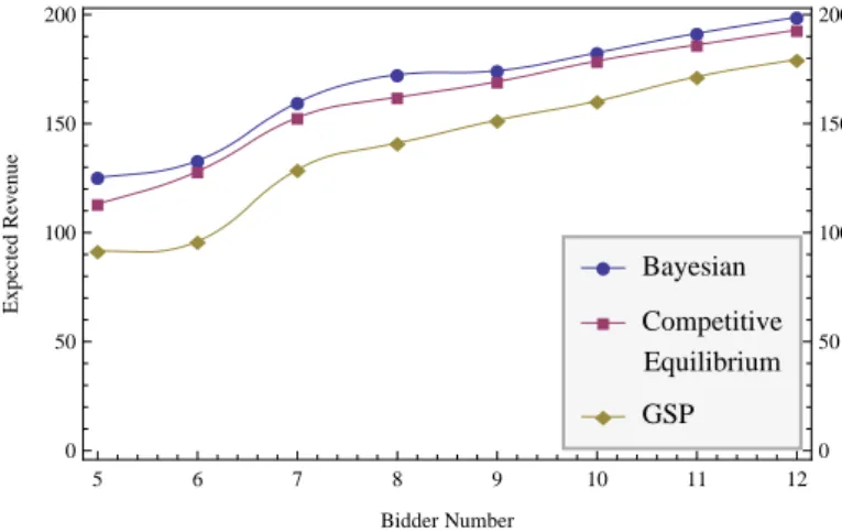
Fig. 2.Simulation results from different mechanisms, bidders’ demand varies in{1,2,3}
Simulation II is for bidders with various demands. With loss of generality, we assume that bidder’s demand D ={d1, d2,· · · , di}, di ∈ {1,2,3}, we assign those bidders’ demand randomly, with equal probability.
Figure 2 shows our simulation results for II when bidders’ demand varies in {1,2,3}, the rank of expected revenue of different mechanisms remains the same as simulation I, From this chart, we can see that Bayesian truthful mechanism and competitive equilibrium get more revenues than generalized GSP.
11
Pseudo-code of Simulation
11.1 Expected Revenue for Bayesian Truthful Mechanism
Suppose with loss of generality,b1> b2> . . . > bn >10, andq1> q2> . . . > qn, letϕi(vi) = 2vi−bi−10.
The following the sub algorithm for finding the allocationsXi whenϕi, i= 1,2,· · · , nare known.
11.2 Revenue from Competitive Equilibrium
ALGORITHM 1:Bayesian Expected Revenue
Input: Demandsdi, qualities(CTR)qj and bidsbi, number of samplesK
Output: Expected Revenue R
Generate uniform distribution forbiasIiuniformly distributed on
Ii= [bi−10, bi+ 10];
Repeat ;
forr= 1,2,· · ·, Kdo Generatevr
i fromIi independently,i= 1,2,· · ·, n;
Calculateϕi(vri) and sort it decreasing order asϕ′i(vri)> ϕ′i+1(vir),i= 1,2,· · ·, n;
Use dynamic programming
g[s, r] = max g[s−1, r] g[s−1, r−ds] +ϕ′s(vsr) ∑r j=r−ds+1qj (13)
By tracking dynamic programming find allocationXi;
CalculateRr=∑ iϕi(v r i) ∑ j∈Xiqj end returnR= 1 K ∑K r=1R r;
11.3 Revenue from generalized GSP 11.4 Revenue from Envy-free Solution Supposeq1≥q2≥q3≥ · · · ≥qn
ALGORITHM 2:sharp
Input: virtual surplusϕi qualitiesqj
Output: Allocationxij
Sort buyersiin decreasing order ofϕi;
g[i, j]← −∞;g[0,0]←0; u[i, j]←0;xij←0;
foreach buyeriwith positiveϕi do
foreach itemjdo
tmp←g[i−1, j−di] + ∑j k=j−di+1ϕiqk; g[i, j]←g[i−1, j]; if g[i, j]< tmpthen u[i, j]←1; g[i, j]←tmp; end end end
g[i∗, j∗] = maxi,j{g[i, j]};
whilei∗>0do if u[i∗, j∗] = 1then
foreach itemkfromj∗−di∗+ 1toj∗ do
xi∗,k←1; end j∗←j∗−di∗; end i∗←i∗−1; end returnx;
ALGORITHM 3:Sub-algorithm for CE denoted by CE(d,q,b) Input: Demandsdi, qualities(CTR)qj and bidsbi
Output: Equilibrium (X,p)
Sort the bidsbiin decreasing order e.g.b1> b2>· · ·> bn;
Use dynamic programming
g[s, r] = max g[s−1, r] g[s−1, r−ds] +bs ∑r j=r−ds+1qj (14)
By tracking dynamic programming find allocationX; Using following LP to settle pricep;
LetTibe any consecutive number ofdislots, for alli∈[n];
max ∑ i∈[n] ∑ j∈Xi pj s.t. pj≥0 ∀j∈[m] pj= 0 ∀j /∈ ∪i∈[n]Xi ∑ j∈Xi (viqj−pj)≥ ∑ j′∈Ti (viqj′−pj′) ∀i∈[n] ∑ j∈Xi (viqj−pj)≥0 ∀i∈[n]
if LP has a feasible solutionthen return (X,p)
end else
return null; end
ALGORITHM 4:Main Algorithm for CE
Input: Demandsdi, qualities(CTR)qj and bidsbi, Accuracyϵ, biding times K
Output: R revenue b1
i =bi,vi=bii= 1,2,· · ·, n.
invoke Sub-algorithm for CE on (d, q, b1), if output is not null then
Suppose the output is (X,p)
calculate the utility for alli. e.g.ui=vi ∑ j∈Xiqj− ∑ j∈Xipj end forr= 1,2,· · ·, Kdo fori= 1,2,· · ·, ndo letMr i =⌊bri/ϵ⌋; fortri =ϵ,2ϵ,· · ·, Mir∗ϵdo
invoke Sub-algorithm for CE on input (d, q,(tri, b r −i))
if the output is not null then Suppose the output is (X,p) Calculate the current utilityu=vi
∑ j∈Xiqj− ∑ j∈Xipj if u > uithen letui=uandbr+1i =t r i,bri =tri. end else br+1i =bri; end end end end Rr=∑jpj end
ALGORITHM 5:Algorithm GSP
Input: Demandsdi, qualities(CTR)qj and bidsbi, Accuracyϵ, biding times K
Output: R revenue b1
i =bi,vi=bii= 1,2,· · ·, n.
Suppose the allocation of GSP isX=sharp(b, q); calculate the utility for alli. e.g.ui=vi
∑ j∈Xiqj− ∑ j∈Xipj forr= 1,2,· · ·, Kdo fori= 1,2,· · ·, ndo letMir=⌊bri/ϵ⌋; fortri =ϵ,2ϵ,· · ·, M r i ∗ϵdo
Suppose the output of GSP on (d, q,(tr
i, br−i)) is (X,p)
Calculate the current utilityu=vi ∑ j∈Xiqj− ∑ j∈Xipjof bidderi if u > uithen letui=uandbr+1i =t r i bri =tri . end else br+1i =b r i; end end end returnRr=∑ jpj end
ALGORITHM 6:Sub-algorithm for EF denoted by EF(d,q,b) Input: Demandsd, qualities(CTR)qjand bidsbi
Output: Equilibrium (X,p)
Sort the bidsbiin decreasing order e.g.b1> b2>· · ·> bn;
Use dynamic programming(similar as sharp)(initial valuesg[0,0] = 0,g[1, r] =−∞, r≤d) g[s, r] = max g[s, r−1] g[s−1, r−d] +bs ∑r j=r−d+1qj (15) By tracking dynamic programming find allocationX;
The payment of buyers areP, wherePiis the payment of buyeri;
Pn=bn ∑ j∈Xnqj, andPi=bi( ∑ j∈Xiqj− ∑ j∈Xi+1qj) +Pi+1fori= 1,2,· · ·, n−1
ALGORITHM 7:Main Algorithm for EF
Input: Demandsd, qualities(CTR)qjand bidsbi, Accuracyϵ, true valuevi, biding
timesK Output: R revenue b1i =bi,i= 1,2,· · ·, n.
invoke Sub-algorithm for EF on (d, q, b1), if output is not null then
Suppose the output is (X,P)
calculate the utility for alli. e.g.ui=vi ∑ j∈Xiqj−Pi end forr= 1,2,· · ·, Kdo fori= 1,2,· · ·, ndo letMir=⌊bri/ϵ⌋; fortr i =ϵ,2ϵ,· · ·, Mir∗ϵdo
invoke Sub-algorithm for EF on input (d, q,(tr i, br−i))
if the output is not null then Suppose the output is (X,P) Calculate the current utilityu=vi
∑ j∈Xiqj−Pi if u > uithen letui=uandbr+1i =t r i,bri =tri. end else br+1i =br i; end end else br+1i =b r i; end end end Rr=∑ iPi end