Financial Institutions and The Wealth of Nations: Tales of Development

T

HE

W

ILLIAM

D

AVIDSON

I

NSTITUTE

Financial Institutions and The Wealth of Nations:

Tales of Development

By: Jian Tong and Chenggang Xu

William Davidson Institute Working Paper Number 672

April 2004

Financial Institutions and The Wealth of Nations:

Tales of Development

∗

Jian Tong

University of Southampton

[email protected]

Chenggang Xu

London School of Economics

[email protected]

First version: December 2000

Present version: December 2003

Abstract

Interactions between economic development andfinancial

develop-ment are studied by looking at the roles of financial institutions in

selecting R&D projects (including for both imitation and innovation).

Financial development is regarded as the evolution of the financing

regimes. The effectiveness of R&D selection mechanisms depends on

the institutions and the development stages of an economy. At higher

development stages afinancing regime with ex post selection capacity

is more effective for innovation. However, this regime requires more

decentralized decision-making, which in turn depend on contract

en-forcement. Afinancing regime with more centralized decision-making

∗_{A previous version of this paper was titled “Endogenous Financial Institutions, R&D}

Selection and Growth.” Discussions with Kenneth Sokoloff, comments from Danny Quah, the participants at the ESEM 2003 Conference (Stockholm) and at a seminar at Southamp-ton, and editorial assistance from Nancy Hearst are greatly appreciated.

is less affected by contract enforcement but has no ex post selection ca-pacity. Depending on the legal institutions, economies in equilibrium

chose regimes that lead to different steady-state development levels.

Thefinancing regime of an economy also affects development dynamics

through a ‘convergence effect’ and a ‘growth inertia effect.’ A backward

economy with afinancing regime with centralized decision-making may

catch up rapidly when the convergence effect and the growth inertia

effect are in the same direction. However, this regime leads to large

de-velopment cycles at later dede-velopment stages. Empirical implications are discussed.

Key Words: development, transition,financial institutions, R&D

JEL Classification: O1, O3, O4, G0, P0, K0

1

Introduction

It has been documented that almost all successful development in history has involved intertwined institutional and technological changes. Moreover, such development is always associated with an economy’s catching up to the more developed economies in terms of wealth and technology. Most promi-nent examples include the contipromi-nental European economies in the 19th cen-tury, Japan after the Meiji Restoration and after World War II, and Korea after World War II.1 Gerschenkron and Cameron, in particular, have inde-pendently observed that the banking systems in continental Europe played an essential role in its catching up in the nineteenth century (Gerschenkron, 1962; Cameron, 1967). Schumpeter (1936) ascertained the relationship be-tweenfinancial institutions and development. He argued that banks play im-1_{There is a substantial literature to support this claim. Due to space limitations we}

portant roles in selecting projects that ultimately affect technological change and economic development.

There is a growing literature that has made great progress in exploring and testing the relationship between institutions and economic development (e.g., King and Levine, 1993; La Porta et al., 1998; Engerman and Sokoloff, 2000; Acemoglu et al., 2002). However, many gaps still remain and many important questions are still being debated. What are the institutional mechanisms that help or hinder technological change and economic devel-opment? How are these mechanisms chosen in the development process?

This paper is an attempt to address these questions with a focus on the

financial institutions. We develop an endogenous growth model in which

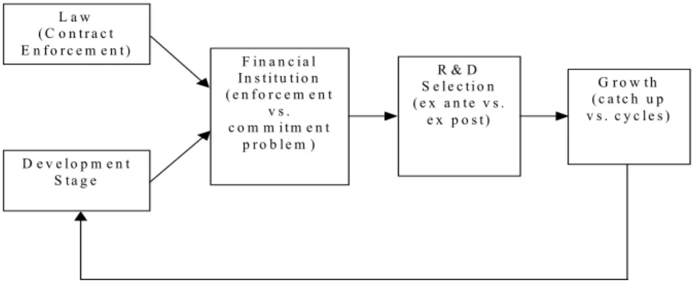
financing mechanisms, development levels, R&D activities, and economic growth are endogenized jointly. Financial development is regarded as an evolution of the financing regimes, together with the economy’s develop-ment level. In our model, R&D is broadly defined to consist of all activities that improve knowledge about technology, including imitation, innovation, and invention.2 Furthermore, exogenously given legal conditions and an endogenously determined development level affect the choice offinancial in-stitution jointly, which in turn determines the R&D selection mechanism and efficiency. As a result, economies develop along different paths. Our theory has implications for how to measure financial development, how to explain existing observations, and what new empirical evidence should be collected. Figure 1 summarizes the basic structure of our model.

In our model we analyze the impacts of project selection mechanisms associated with different financial institutions on development. We also

2

Because our definition of R&D, the usual R&D statistical measurements cover only part of the R&D in our model.

L a w ( C o n t r a c t E n f o r c e m e n t ) F i n a n c i a l I n s t i t u t i o n ( e n f o r c e m e n t v s . c o m m i t m e n t p r o b l e m ) D e v e l o p m e n t S t a g e R & D S e l e c t i o n ( e x a n t e v s . e x p o s t ) G r o w t h ( c a t c h u p v s . c y c l e s )

Figure 1: A model of endogenized institution, R&D, development level, and growth

explore how the development level determines the choice offinancial institu-tion. Project selection mechanisms are related to the incentives provided by thefinancial institutions to entrepreneurs for R&D. These incentives include ‘carrots’ to reward entrepreneurs and ‘sticks’ to prevent cheating. Our model focuses on the latter because, in our view, these are particularly important in dealing with the following important features of R&D: a) the uncertainty of R&D projects for innovation/invention can be very high such that essen-tial knowledge for a project is only known ex post; whereas the uncertainty for imitation is low since reasonably accurate information can be collected ex ante; b) individuals with R&D ideas usually do not have the resources tofinance projects so they need outside investment; c) entrepreneurs have informational advantages over projects that they work with, and with these advantages they may benefit by cheating on the worth of the projects.

Cheating can be deterred if it is punished whenever it is revealed. More-over, an effective deterrence is a better R&D selection mechanism for in-novation. However, such punishments can be enforced only when they are consistent with thefinanciers’ ex post calculations. But the commitment to

ex post punishments depends on the financing mechanisms. Two types of

financial institutions are studied: regimes with more centralized decision-making,3 _{reflecting the conglomerates’ internalfinancing, ‘relation-basedfi}

-nancing’4 or a centralized finance system in reality; and regime m with more decentralized decision-making, reflecting venture capital or syndicated

financing in reality. The institutions of regime s have no commitment for ex post punishment, i.e., they are associated with a soft budget constraint problem (SBC);5 whereas regime m is committed to punishing cheating ex post, i.e., it is associated with hard budget constraints.6

An alternative approach to deal with the R&D-related incentive problem in our model is to select R&D projects ex ante. Associated with the above-mentioned R&D feature a), the effectiveness of pre-screening R&D depends on the information available ex ante. The more novel the project, the less information available to make ex ante judgments; whereas it is much easier to evaluate projects that have marginal novelty, such as those involving technology imitation. Thus a relatively backward economy will benefit from imitation which reduces the problems of cheating in R&D when projects are selected ex ante. We model the degree of backwardness of an economy as 3_{Whenfinancing decisions are concentrated in the hands of onefinancier we regard the}

correspondingfinancial institution as a single-financierfinancing regime, i.e., regimes.

4

The term is borrowed from Rajan and Zingales (2003).

5

An observable indication of the existence of a substantial SBC problem in an economy is a large amount of non performing loans (NPL), such as those in transition economies and in Japan during the last decade. The NPL/GDP ratio in Japan was 15.3% in 2001, far higher than any other developed economy.

6

For the contractual foundations of the commitment problems associated with cen-tralized and decencen-tralizedfinancing regimes, see Dewatripont and Maskin (1995); for the contractual foundations of the commitment problems associated with differentfinancing regimes in market economies, see Huang and Xu (1998, 2003).

the distance from that economy to that of the world frontiers.

Regime m institutions are more efficient in innovation; whereas under certain conditions regimes institutions can be more efficient in technology imitation although they are less efficient in innovation. We predict a condi-tional convergence such that in equilibrium, economies with stronger legal institutions chose a regimemthat leads to higher steady-state development levels, whereas those with weaker legal institutions chose a regimes. Since ex ante R&D selection is less effective in solving incentive problems when the development level is higher and imitation opportunities diminish, this leads to lower steady-state development levels for regimes.

Another major contribution of our work is to analyze the catch-up namics by decomposing the impacts of institutions on the development dy-namics into a ‘convergence effect’ and a ‘growth inertia effect.’ The magni-tude and the direction of the two effects govern the development dynamics of an economy. The key factor that determines the magnitude of each effect is what we discover from the model: the ‘inertia factor’ of the economy. The ‘inertia factor,’ a measure of the ability to reserve the momentum of growth performance, is determined by institutions. Moreover, it is empiri-cally observable as the auto-correlation coefficient of the growth rate. At a catching-up stage, the convergence effect and the growth inertia of an econ-omy are in the same direction. Thus, a backward econecon-omy with a higher ‘inertia factor’ will catch up faster. However, when an economy’s develop-ment level is close to its steady state, a higher ‘growth inertia’ may make the economy prone to growth cycles.

Among other factors, the ‘inertia factor’ of an economy is affected by how much ex ante R&D selection is used in the economy, which in turn is determined by the financing regime. In general, the ‘inertia factor’ under

regimem is smaller than that under regime s.

Together with the results of howfinancing regimes determine their steady state, our theory predicts that the institutions of regimeslead to a fast catch up when an economy is at an earlier development stage; however, it is likely to fall into growth cycles around the relatively low steady-state develop-ment levels. In contrast, although the institutions of regime m may have higher steady-state development levels associated with more stable catch-up patterns, their catch-up speed may vary depending on the legal institutions. These predictions shed light on why economies associated with some fi -nancial institutions, such as centralizedfinancing or ‘relationshipfinancing,’ catch up quickly at earlier stages but encounter serious problems later even when investments in R&D are high. Our theory is consistent with some observed development patterns, including the rise and fall of centralized economies.

The structure of the paper is as follows. Section 2 presents some moti-vating observations and discusses the related literature. Section 3 sets up an endogenous growth model, focusing on the role of financial intermedi-ation on R&D project selection. Section 4 describes equilibrium financing regimes, the R&D level, the steady-state growth rate, and the steady-state development level. Section 5 explores the catch-up dynamics by which an economy converges with or diverges from its steady-state path. Section 6 briefly provides suggestive empirical evidence; moreover, policy implications of the theory are demonstrated through simulations. Finally, section 7 offers some conclusions.

2

Catching-up Patterns and the Related

Litera-ture

In this section we present some observations motivating our theory. Wefirst briefly compare the development paths in the last half-century between some West European economies, where the financial institutions were relatively closer to regime m in our model, and some Central and Eastern European (CEE) economies that were under centralizedfinancial systems prior to the 1990s, thus representing an extreme case of regimesin our model. It is well recognized that a centralized financial system, where all national financial resources are concentrated in state banks, creates the so-called ‘soft-budget constraint’ syndrome that is one of the most serious problems in central-ized economies (Kornai, 1979; Dewatripont and Maskin, 1995; for recent surveys, see Maskin and Xu, 2001; Kornai, Maskin, and Roland, 2003). However, the rise of the centralizedfinancing regimes is puzzling, i.e., they appeared to catch up quickly at earlier development stages, given that the SBC is inefficient. Moreover, the fall of the centralized financing regimes is also puzzling, i.e., they experienced a reversed catch-up pattern at later development stages, given that the negative experience was associated with their heavy investments in R&D (both in monetary and in human capital terms). Our model provides an explanation for the rise and fall of the SBC economies together with their R&D activities.

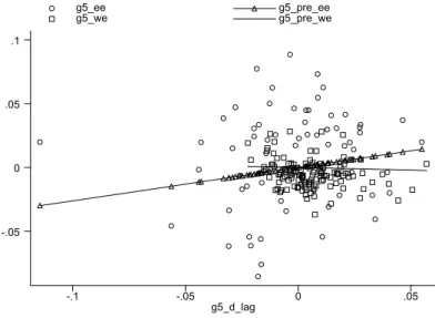
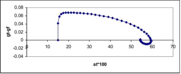
Presenting the growth rate differences with those of the world frontiers by the vertical axis, Figure 7 shows the development paths of four Western European economies (Austria, Belgium, France, and Italy) for the period from 1950 to 2000 based on a five-year average (data source: Madison,

2003).7 A regular catching-up pattern consistent with the predictions of our model (Fig. 5) seems to emerge such that all these economies had catch ups before the 1980s; thereafter, their catch ups ended with small growth cycles when their development levels were close to that of the frontiers (from 70% to 81% of the U.S. level).

In comparison, Figure 8 illustrates the catch-up patterns of some CEE economies (Hungary, Poland, Romania, and the USSR), which appear to be consistent with the predictions of our model (Fig. 6). Although associated with the SBC problem, all the CEE economies underwent fairly rapid catch ups in their earlier stages (before 1975), together with the rapid adoption of new technologies.8 _{However, the catch ups all ended with large growth cycles}

when their development levels reached one-third that of the U.S. level.9 The reversed catch-up trend since the 1980s seems to confirm our prediction that these economies will decline on a large scale after overshooting.

7_{The development path of each economy is plotted in a development level growth rate}

space so that the development level and growth rate of each economy can be compared with those of the world frontiers, which are proxied by those of the U.S., given that the data come from the latter half of the twentieth century. The development level relative to that of the world frontiers (hereafter referred to as the development level) is measured by the ratio of the per capita GDP of this economy to that of the U.S. It is presented by the horizontal axis.

8_{For example, except for in syntheticfibers, the USSR adopted major new technologies}

that were introduced in the 1940s and 1950s (oxygen steel making, continuous steel casting, syntheticfibers, polyolefins, HVAC [300 kv and over], nuclear power, NC machine tools) around the same time as the UK, FRG, and Japan (Bergson, 1989, Table 10, p.124).

9

The data reflecting the collapse of the centralized economies over the last decade are the last two points on the curves. The basic development pattern of these economies will not change qualitatively if these data are excluded. The only reason for including the data for the period from 1990 to 2000 is to present the data in the same way as those for the West European economies.

With respect to the mechanism for the fall of the centralized economies, we predict an increase in R&D expenditure when the development of regime

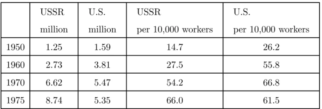
sbegins to decline. Our explanation focuses on the failure of thefinancing regime to deal with R&D. A corresponding fact is that when the catch-up re-versal occurred, the R&D (both in the civilian and military sectors) in these economies was among the highest in the world (Tables 1-3). Specifically, beginning in 1975 R&D intensity in the USSR was the highest in the world both in monetary terms and in terms of human capital inputs: compared with the U.S., the R&D intensity and the number of scientists employed in R&D in the USSR in 1975 was about 47% and 63% higher respectively (Table 1 and 3).10

Moreover, our theory seems consistent with much of the existing evi-dence in the recent literature. Rajan and Zingales (1998, RZ hereafter) make major progress in confirming the causality between financial and economic development after the pioneering work by King and Levine (1993) which established positive correlations between the two developments. Interpret-ing regime m/s in our model as external/internal financing11 and relating our model to RZ’s work in broad terms, our model predicts that external

financing is essential for the growth of industries with technologies close to 1 0

For all countries under comparison, the R&D includes both the civilian and military sectors. Great care has been taken to rely on the most prominent experts in thefield for the source of our data: we use Madison for the GDP/GNP data; and Bergson and Hanson for the R&D data.

1 1

Indeed, regimemin our model reflects such externalfinancing as venture capital, syn-dicated loans, or other ‘market-based institutions’ that are able to solve the commitment problem; and regimesreflects internalfinancing within large conglomerates,financial in-stitutions with strong government intervention, or ‘relation-based inin-stitutions’ that are unable to solve commitment problems.

the frontiers of knowledge.12 In contrast, internal financing may be more efficient for industries with technologies far from the frontiers of knowledge. The data in RZ show that industries involving more ‘new technologies,’ such as pharmaceuticals, electronics, and computers, are more dependent on ex-ternal financing for growth. In contrast, industries involving ‘traditional technologies,’ such as iron and steel, auto vehicles, and machinery, are much less dependent on external financing for growth (the industries least de-pendent on externalfinancing in RZ are tobacco, pottery, and leather) (RZ, 1998, Table 1). Indeed, in the U.S. an overwhelming proportion of the most innovative R&D projects in ‘new technologies’ werefinanced by syndicated venture capital (Gompers and Lerner, 2001), whereas most innovations in-volving ‘traditional technologies’ in all developed economies were created by in-house R&D.13

A high (or low) bank concentration in an economy may make thefi nanc-ing in that economy closer to regimes(orm). If we interpret thefinancing regimes in this way, our theory implies that a higher bank concentration may be beneficial for catching-up economies, whereas a lower bank concentration may be more efficient for industries at technological frontiers in developed economies. Carlin and Mayer (2003) found that bank concentration is

neg-1 2

A fundamental feature of the frontiers of knowledge in our model is the degree of uncertainty in innovation. This can be very different from merely being the most advanced in thefield. For example, inventing a new drug requires the frontiers of knowledge in biology and involves high uncertainties, whereas innovations to improve the quality of steel may not involve very high uncertainties.

1 3_{The financing regimes in the U.S. before the mid-nineteenth century (the early}

catching-up stage) may further illustrate this point. At that time New England banks effectively facilitated development. Instead of being commercial banks, they werefi nan-cial arms of kinship networks that lended mainly to insiders (Lamoreaux, 1986).

atively correlated with growth in developed OECD economies: a lower bank concentration is associated with higher R&D shares and faster growth of externally financed industries. However, for countries at earlier stages of development, the converse result is found, such that a high bank concen-tration is associated with faster growth (Carlin and Mayer, 2003, Tables 6 and 8). Moreover, our results about how contract enforcement affects de-velopment are consistent with empirical evidence that shows that economies with stronger legal institutions have betterfinancial development and better economic development (La Porta et al., 1998).

Using data from 72 countries for the 1978-2000 period, a discovery by Demetriades and Law (2004) also fits well with our model. They found thatfinancial development has significant effects on growth; the effects are stronger for economies with better institutions; moreover, for underdevel-oped economies, the quality of the institutions has a dominant impact on growth. To link their discovery to our model, we need to mention the follow-ing features of their data: a) their institutional quality data are essentially related to the contract enforcement in our model; b) most underdeveloped countries sampled in their study havefinancial institutions closer to regime

m in our model.

Our theory is developed based on two strands of literature. The first is the R&D-based growth literature (Romer, 1990; Grossman and Help-man, 1991; Aghion and Howitt, 1992). The second is the literature on the commitment problems offinancial institutions (or the theory of soft budget constraints) (Kornai, 1979; Dewatripont and Maskin, 1995; Huang and Xu, 2003), which provides the contractual foundation for our growth model.

Qian and Xu (1998) develop the idea that financing regimes are used as different R&D selection mechanisms dealing with different types of R&D

projects. However, the implications for growth or development are only mentioned are not modeled. In an endogenous growth model Huang and Xu (1999) study howfinancial institutions affect growth through their R&D selection mechanisms. Although this paper notes the implications of R&D selection mechanisms for catch-up’s economies and for economies at other development stages, the discussions are very brief and there is no full-fledged model of these issues. Moreover, since the HX model takes the financial institution as exogenous and the analysis is restricted to steady states, it is unable to make most of the predictions generated by our model.

Recent work by Acemoglu, Aghion, and Zilibotti (2003) studies the selec-tion of managers related to the growth offirms using an investment-based strategy and an innovation-based strategy with an emphasis on competi-tion. Their model creates multi-equilibria and a development trap in that context. However, they do not focus on the relationship between fi nan-cial development and economic development, and they do not derive large growth development cycles. Accordingly, their model does not make predic-tions related to the observapredic-tions that we discuss here (e.g., Fig. 7 and 8; RZ, 1998; Carlin and Mayer, 2003, etc.).

With respect to our contribution to growth cycles, Matsuyama (1999, 2001) studies possible growth paths cycling between a non-innovative (com-petitive) phase and an innovative (monopolistic) phase due to the interac-tion between innovainterac-tion and the accumulainterac-tion of capital. In our model we have imitation vs. innovation, and the growth cycles are determined by the

3

The Model

Our model focuses on the impacts of institutional solutions to incentive problems in R&D on long run growth. In our theory, the Romer model (1990) is the benchmark model whereby if there is no capital requirement or information asymmetry in R&D, our model becomes a discrete-time version of the Romer model. In the following, we start from the benchmark model, and then add institutional features to the model.

3.1

Production

In our model, consumers are risk neutral and infinitely lived. The represen-tative consumer’s maximization problem is,

maxP∞_τ=t cτ

(1+ρ)τ−t

s.t.:bτ+1 =wτ+bτ(1 +rτ)−cτ,

(1)

wherecτ is consumption, and wτ is labor income, bτ is the holding of bond

with interest raterτ,ρis the discount rate; in equilibrium, rτ =ρ.

Production in this economy is standard which consists of a final good sector and an intermediate good sector. The final good sector is perfectly competitive and it has a Cobb-Douglas technology with intermediate inputs

xit and labor input L1t, such that the output is

Yt=L11−tα At X i=1 xα_it, 0<α<1. (2) Thefirm’s program is max xit,L1t à L1₁−_tα At X i=1 xα_it−(1 +ρ)pitxit−L1twt ! ,

wherepitis the price of intermediate good xit,andwtis the cost of labor at periodt. Thefinal good producers pay the intermediate goods producers at the beginning of each period to get the inputs, and sell their own products and pay their workers at the end of each period. The optimal demands for intermediate goods and labor are:

xit =α Yt (1 +ρ)pit xα it PAt i=1xαit (3) and L1t= (1₋α)Yt wt (4) The producer of intermediate good i is a monopolist with the following profit maximization program:

max pit,xit πit = max pit,xit{ pitxit−xit} (5) s.t. : αL1₁−_tαxα_it−1 = (1 +ρ)pit And its solution is

pit=

1

α. (6)

The solutions for all intermediate goods producers are symmetric, so the subscriptican be dropped. Then we have,

xt= α2Yt At(1 +ρ) =α1−2α _{(1 +ρ)}− 1 1−α_{L1t (7)} pt= 1 α (8) πt= (1−α)α 1+α 1−α _{(1 +ρ)}− 1 1−α_L 1t (9)

wt= (1₋α)Yt L1t (10) and Yt At =α12α−α(1 +ρ)− α 1−αL_1t (11) and L1t= (1₋α)Yt wt (12) Define w¯, wt

At, the ratio of wage-knowledge stock, we have

¯ w= wt At = (1−α)Yt L1tAt = (1₋α)α12α−α _{(1 +ρ)}− α 1−α_. wt=Atw¯ forL1t>0 and wt is undefined when L1t= 0.

Then, the profit for every intermediatefirm in each period is, πt=

αw¯

1 +ρL1t. (13)

Denoting the steady stateL1t asL1, the steady state xt and πtare

x=α1−2α _{(1 +ρ)} − 1 1−α_L1 and π = αw¯ 1 +ρL1. (14)

The number of new intermediate products introduced in periodt+ 1 as a result of R&D activities att is determined by the productivity efficiency of R&D sectorδ, labor input in R&D sectorL2t,14 and the knowledge stock

At, i.e., 1 4

Here, a crucial departure from the standard Romer model arises. As will be elaborated upon the next subsection, each R&D project needs capital inputs to complement one unit of labor input.

At+1−At=δL2At, (15) where, L2t, the labor input in the R&D sector, is determined by the labor market clearing condition

L2t=L−L1t. (16)

3.2

Financial Intermediation and R&D

In our model, we assume that R&D is uncertain and is subject to incentive problems, whereas all other productions are certain. A major function of financial intermediaries is to solve the entrepreneurs’ incentive problems when theyfinance uncertain R&D projects.

The incentives to be provided involve ‘carrots’ to reward entrepreneurs and ‘sticks’ to prevent cheating. The latter issue is particularly serious and difficult for R&D due to the following features of R&D: a) individuals with R&D ideas usually have no wealth tofinance projects such that they need others’ wealth as investment; b) R&D projects can be highly uncertain such that ex antefinanciers may not be able to know which project is worth doing. Although ex ante it seems to be obvious that cheating can be deterred by severe punishment once it is revealed ex post, such punishments will be enforced only when the ex post punishment is consistent withfinanciers’ ex post benefits. That is, only when ex post punishment is time consistent for thefinanciers can the incentive problem be solved properly and this depends on the financial institutions.

To deal with the R&D incentive problem in a growth model, in our econ-omy there are always some consumers who can generate innovative ideas during every period following an independent identical stochastic

distrib-ution. The consumers with innovative ideas will become entrepreneurs if their ideas arefinanced. The i.i.d. assumption implies that no entrepreneur can automatically continue to be an entrepreneur during the next period.

We assume that there are two possible types of every project proposed by an entrepreneur: a good type and a bad type. The returns of the two types of projects are the same — the present value of profits,δAtP∞τ=t+1(1 +ρ)−

(τ−t)_π

τ

(notice thatδL2At is the number of new R&D outcomes introduced in pe-riodt+ 1and each R&D project uses one unit of labor). But the costs of the two types of projects differ. For a project being carried out in periodt, a good type takes two stages to complete, requiring (capital) investmentsI1t andI2t; and it is profitable. However, a bad type takes three stages to com-plete requiring (capital) investments I1t, I2t and I3t and it is unprofitable. Moreover, we also assume that all early stage investments to a bad project

I1t and I2t are sunk, such that a bad project’s liquidation value at stage 2 is zero. The magnitude of each investment is given byIit =IiAt, whereIi is constant, for i= 1,2and 3.

With respect to information, when a project is proposed by an entrepre-neur, no one (including the entrepreneur) knows the type of each project, although it is a common knowledge that the probability that it is a good (bad) type is q (q¯,1₋q). Facing unknown-type R&D projects and po-tential losses associated withfinancing bad type projects,financiers may do better to select projects ex post by eliminating bad ones once the projects’ types become known, i.e., if the financiers commit not to make last stage investment I3t. However, this ex post selection mechanism may not be

im-plemented if investingI3t can make a bad project ex post profitable, unless investingI3tmakes an ex post loss due to some additional transaction costs. To study R&D selection mechanisms, we model two alternativefinancing

regimes: a multi-financier financing regime (regime m, with a dispersed claim structure) and a single-financier financing regime (regime s, with a concentrated claim structure). We suppose that a transaction cost

Ft=F At

is incurred whenever a project is to be re-financed by multi-financiers at stage 2, where F _∈ R+. Ft may be justified as a negotiation cost due to the conflict of interests and asymmetric information among the co-financiers under the regime m. When a project is financed by regime s, this trans-action cost does not appear.15 In the following we summarize our major assumptions in an intuitive way; formal expressions of these assumptions can be found in Appendix A.

A-1 Financing a bad project is ex ante unprofitable.

A-2 Given that earlier investments are sunk,financing a bad project at its last stage is ex post profitable.16

A-3 With the transaction costFt, financing a bad project at its last stage is ex post unprofitable.17

To describe the incentive problems in financing R&D, we illustrate the stages of R&Dfinancing in periodt as follows:

1 5

This costFtcan be regarded as a reduced form of the endogenized renegotiation costs

in Huang and Xu (1998, 2003). Moreover, there is a literature on different reasons why costs will be higher when there are more parties involved (e.g., Dewatripont and Maskin, 1995; Bolton and Scharfstein, 1996; Hart and Moore, 1995).

1 6

This assumption is a variation of similar assumptions made by Dewatripont and Maskin (1995); Qian and Xu (1998).

Stage 0 Financiers choose thefinancial institution — regimesorm. Poten-tial entrepreneurs propose R&D projects tofinanciers under a chosen regime when no one knows the types of proposed projects. Based on ex ante selection, which is to be analyzed in the next subsection, fi -nanciers make take-it-or-leave-it contract offers to the proposers of the chosen project. If a contract is signed, the project proposer becomes an entrepreneur and thefinancier(s) investI1tunits of money into the project during stage 1. Stage 1 takes no time and requires no labor input.18

Stage 1 An entrepreneur learns the type of the project proposed. How-ever, the financier(s) still does (do) not know the type of the project and stage 2 of R&D is launched (unless a project is stopped by the entrepreneur), which requiresI2t units of capital and one unit of labor inputs. If the entrepreneur stops the project, he gets a low private benefit b1>0.

Stage 2 All good projects are completed, thus the types of the projects be-come common knowledge. For a good project, all thefinancial returns go to thefinancier(s) and the entrepreneur gets a high private benefit of bg. All bad projects are incomplete, thus they have no return and their liquidation values are zero. Thefinancier(s) decide either to con-tinue, or to liquidate them. If a project is liquidated the financier(s) get(s) zero return and the entrepreneur loses, i.e., the private benefit 1 8_{Relaxing this simplification assumption will not change the model qualitatively. A}

justification for the assumption is the following. Suppose testing a proposed idea is quick, then the time spent on it can be ignored. Moreover, suppose the number of people working on it can be very small, then compared with the later stage, it is small enough to be ignored.

isb2 < b1. If it is to be reorganized,I3t will be invested. To simplify the model, we assume no further labor input is required to continue.

Stage 3 Bad projects are completed. All the financial returns go to the

financier(s) and the entrepreneur gets a moderate private benefit,bb ∈

(b1, bg).

Given assumption A-2, financiers under regimeswill continue to invest in bad projects at stage 2. Anticipating this, entrepreneurs with bad projects will lie at stage 1 to benefit from continuing bad projects. However, following A-3,financiers under regimemwill liquidate bad projects at stage 2. Facing the credible threat of liquidation of bad projects at stage 2, entrepreneurs endowed with bad projects will stop bad projects “voluntarily” at stage 1 to avoid heavier losses later. These results are summarized in the following.19

Lemma 1 : Under regime s all bad projects will not be stopped, i.e., there

is a pooling equilibrium. Under regime m all bad projects will be liquidated

at date 1, i.e., there is a separating equilibrium.

Proof. See Appendix A.

The above lemma shows that through its commitment to liquidate bad projects at date 2, the decentralized nature of regimem provides incentives for entrepreneurs to honestly disclose information about the quality of the projects. In contrast,financial systems where key decisions are made by a single agent (regimes) do not have a commitment to liquidate bad projects ex post. Without a commitment entrepreneurs under this regime will hide bad news about their projects. Examples of regimem, or a dispersed claim

1 9

There are other possible contractual foundations that we can use to derive the Lemma1, such as internal influence activities within regimes(Milgrom, 1988).

structure, are syndicated venture capitalfinancing and decentralized fi nan-cial markets such as equity markets; whereas examples of regimes include largefirms’ internal financing (e.g. conglomerates) or in-house R&D; a cen-tralized economy is an extreme example (see Dewatripont and Maskin, 1995; Qian and Xu, 1998).

Regime m involves multi-party contracts. Thus, law enforcement such as contract enforcement, accounting standards, etc. will affect its operation. To capture this, we suppose that when a project is to be financed at stage 0, regimem will involve a transaction cost σF At,σ ∈[0,1]when a project is started to align the interests of investors and entrepreneurs. In short, we callσ an institutional cost. This institutional cost σ reflects the degree of imperfection of the legal infrastructure with respect to the costs involved in multi-party contracts. In an economy with perfect law enforcement,σ = 0; but in an economy with imperfect legal institutions, σ >0 ; moreover, the more imperfect the legal institutions the higher σ.20

With respect to the ‘waste’ caused by bad projects in the two regimes, in the benchmark case of regime m (i.e. σ = 0), the present value of ex-pected ‘waste’ for each complete project due to liquidating a bad project is (1₋q)I1

q. In comparison, under regime s the present value of the ex-pected ‘waste’ due to extra costs involved in the final stage of financing is

(1₋q) I3

1+ρ. In this paper we make an assumption that regimeshas higher

‘waste’ than regimem. Formally we have the following. A-4: q I3

1+ρ > I1 (benchmark regimem waste less than regimes).

2 0

This transaction costσ or σF At can be seen as a reduced form of endogenized law

enforcement cost in Xu and Pistor (2002). The assumption that regimesdoes not incur cost σ is not only a simplification but also captures the idea that a regime s, such as conglomerates, is an institutional substitute when the market is less developed.

Furthermore, we assume that to produce intermediate goods from a com-pleted R&D project takes no time. Although it is a simplification assump-tion, a plausible example is that of producing a software package in a large scale when the code is there. Finally, we assume that the law of large numbers applies whenever appropriate. Therefore, we use mathematical expectations to replace the average of samples throughout the rest of the paper.

3.3

Pre-screening and Development Level

At its best, ex post selection is at the expense of I1; at its worst, it does

not exist (in regimes). As an alternative R&D selection mechanism, in our modelfinanciers also select projects ex ante, which we call “pre-screening”. This also captures important features of technology imitation. We assume that the effectiveness of ex ante project selection depends on the quality of ex ante information on R&D projects, which is determined by how far an econ-omy is from the technology frontier. Supposedly, imitation-featured R&D projects (e.g., reverse engineering, etc.) are less uncertain and it is easier to make ex ante judgments about the projects; then a backward economy may rely more on ex ante selection, which allows for trying new technologies at a lower cost.21

Formally, we suppose that by investingκt, a prior signal can be collected about the quality of a project before starting it. The precision of the signal, i.e., the probability that a signal is correct, isθ, where θ_∈£1₂,1¤. We also suppose that the pre-screening cost increases in the development level and in the pre-screening precision. That is, we assume κt =κ(at,θ)At, where 2 1_{This approach captures the Gerschenkron effect of the ‘advantage of backwardness’}

at , _AAt

f t is the relative development level of an economy and Af t is the

world frontier of knowledge stock. Af t grows at a constant rategf, which is to be determined endogenously. We make the following assumption about the properties of the pre-screening cost functionκ.

A-5: κ = λ(at)ψ(θ) where, ψ ¡₁ 2 ¢ = 0,ψ(1) = _∞, ψ0(_·) > 0,ψ00(_·) > 0;22 λ(0) = 0,λ0(_·)>0,λ(_·)_≤ 2¯qI1 ψ0₍1 2) .23

4

Equilibrium

4.1

Endogenous Financing Regime

We model a continuum of economies in the world with σ _∈ [0,_∞). For any periodtat stage 0, after receiving R&D proposals from entrepreneurs,

financiers choose the optimal financing regime and pre-screening precision {ζ,θζ} to maximize the expected net present value (NPV) of the projects

they finance, where ζ is the regime variable, ζ _∈{m, s_}, and θζ is the

pre-screening precision under a chosen regimeζ. In the following, we analyze the twofinancing regimes, and then we look at how at the equilibriumfinancing structure and the equilibrium pre-screening precision.

2 2_{One example which satisfies these conditions isψ(θ) =}θ−12

1−θ.

2 3_{When this upper bound is respected, the equilibrium levelθ is an interior solution,}

i.e., some pre-creening is desirable regardless of the country characteristics and the stage of development.

For a projectfinanced under regime s, the expected NPV is EN P V s = qθs à ∆At+1 L2 ∞ X τ=t+1 (1 +ρ)−(τ−t)πτ−I1t−I2t− wt 1 +ρ ! + ¯ q¯θs à ∆At+1 L2 ∞ X τ=t+1 (1 +ρ)−(τ−t)πτ−I1t−I2t− I3t 1 +ρ− wt 1 +ρ ! −Atλψ(θs) = qθs à δ ∞ X τ=t+1 (1 +ρ)−(τ−t)πτ−C¯s ! At, ifL1t>0, (17) 24_whereqθ s,qθs+ ¯q¯θs and ¯ Cs , λψ(θs) qθs +I1+I2+ ¯ w 1 +ρ+ ¯ q¯θs qθs I3 1 +ρ (18)

is the expected cost of completion of one project. (Note: if L1t = 0, then

wt6= ¯wAt, i.e., the wage rate is not determined by thefinal good sector.) Similarly, for a project financed under regimem, the expected NPV is

EN P V m=qθm à ∆At+1 L2 ∞ X τ=t (1 +ρ)−(τ−t)πτ −I1t−I2t− wt 1 +ρ−σFt ! −q¯¯θm(I1t+σFt)−Atλψ(θm) = qθm à δ ∞ X τ=t+1 (1 +ρ)−(τ−t)πτ−C¯m ! At, ifL1t>0, (19) 25_where ¯ Cm , λψ(θm) qθm +qθm+ ¯q¯θm qθm (σF+I1) +I2+ ¯ w 1 +ρ (20)

is the expected cost of completion of one project. In a competitive capital market only the most efficient financing regime survives. The following result reflects this intuition.

2 4_{For the corner solution that L}

1t = 0 the condition is EN P V s = qθs ³ δP∞_τ=t+1(1 +ρ)−(τ−t)πτ−C¯s+ ³ wt At −w¯ ´´ At. 2 5

For the corner solution that L1t = 0 the condition is EN P V m =

qθm ³ δP∞_τ=t+1(1 +ρ)−(τ−t)πτ−C¯m+ ³ wt At −w¯ ´´ At

Proposition 2 With free-entry in the capital market, the equilibrium fi -nancing regime minimizes the expected capital cost of a completed project,

i.e., at equilibrium a regime is chosen such that(ζ∗,θ∗) = arg min©minθsC¯s,minθmC¯m

ª

.

Proof. Thefinanciers choose the optimal selection regime(ζ,θ)to maximize the expected NPV of the projects they finance, i.e., to solve the following program: max ζ,θ EN P V = max ½ max θs EN P V s,max θm EN P V m ¾ . (21)

Given free entry into the capital market, a break-even condition ensues, i.e.,

maxζ,θEN P V = 0. (Otherwise, an efficient outside financier would find it profitable to enter, or an inside financier would find it profitable to quit.) Using eq. (17) and (19), it is easy to verify that

δ ∞ X τ=t (1 +ρ)−(τ−t)πτ = min ½ min θs ¯ Cs,min θm ¯ Cm ¾ forL1t>0,

26_{and arg min}©_min

θsC¯s,minθmC¯m

ª

is the solution to the program (21). We define the minimum expected cost of completing a project under regime s as C¯_s∗ , minθsC¯s, the minimum cost under regime m as C¯m∗ ,

minθmC¯m, and the cost at equilibrium as C¯∗ , min

©_¯

C_s∗,C¯_m∗ª. Then applying Proposition 2, we have the following result.

Proposition 3 IfC¯_s∗<C¯_m∗, then the equilibriumfinancing regime is regime

s; if C¯_s∗ >C¯_m∗, then the equilibrium financing regime is regimem.

2 6

For the corner solution that L1t = 0 the condition is δP∞_τ=t(1 +ρ)−(τ−t)πτ =

min©minθsC¯s,minθmC¯m ª

+³wt

At −w¯ ´

We denote the optimal pre-screening precision under the two regimes as θ∗_s and θ∗_m respectively, and define the optimal average pre-screening costs under the two regimes asK∗

s , λψ(θ∗s) qθ∗s+¯q¯θ∗s and K∗ m, λψ(θ∗m) qθ∗ m respectively. The

following Lemma shows comparative statics with respect to the institutional cost σ. (For other comparative statics of the model, please see Lemma 25 and 26 in Appendix B.) Lemma 4 dC¯s∗ dσ = 0, dθ∗s dσ = 0 and dK∗ s dσ = 0; dC¯∗ m dσ > 0 and ∂θ∗m ∂σ > 0 and dK∗ m

dσ >0 for λ>0. Moreover, ifσ= 0, then C¯s∗ >C¯m∗ for λ>0.

Proof. See Appendix B.

This lemma suggests that ceteris paribus under regime m, with a high σ thefinanciers will spend more on screening and achieve a higher pre-cision, and the expected capital cost of R&D will be higher. In contrast, under the regimes, the change of institutional costσ has no impact on pre-screening. The last part of the lemma establishes the benchmark case when there is no institutional cost.

Based on the above discussions, the following result demonstrates the determinants of regime choice.

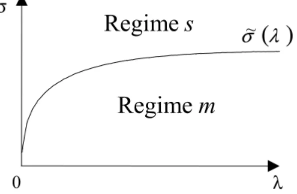
Proposition 5 For λ(a) > 0, there exists a threshold σ˜(λ) > 0 such that

regime sis chosen if and only if σ >σ˜(λ).

Proof. See Appendix B.

The following Figure 2 illustrates Proposition 5. In the figure, a σ˜(λ)

curve partitions the (λ(a),σ) space into two regions: in the upper region regime s prevails; in the lower region, regime m rules. It shows that the choice of financing regime is jointly determined by the exogenous ‘institu-tional cost’σand the relative development levelathroughλ(a). For a given

development levela, orλ(a), when the institutional cost is high in compar-ison with the threshold valueσ˜, at equilibrium regimeswill be chosen; but if the institutional cost is lower thanσ˜, regimem will be chosen.

λ

σ

0

Regime

m

Regime

s

_{( )}

λ

σ

~

Figure 2: Endogenous financial regimes

4.2

Growth

In order to establish the foundation for examining how growth andfinancing regimes interact, wefirst establish the laws of motion, and then characterize the steady state of the system. A complete characterization of the dynamics of the growth paths is in Section 5.

4.2.1 Growth Equations

Letgt, At+1−_AtAt be the rate of growth (of knowledge stock) in period t. We suppose that there is free entry into the R&D sector and the capital market. Focusing on interior solutions that 0 < gt <δL, the number of completed projects in each period is determined by the following arbitrage condition (in equilibrium the expected cost of capital is the same as the asset value of

a completed project):27 δ ∞ X τ=t+1 (1 +ρ)−(τ−t)πτ | {z }

PV of profit from completing a project =

costs of completing a project

z }| {

¯

C∗(λt) (22)

whereπτ is the expected profit per product in period τ.28

From the difference in the arbitrage conditions for period t and period

t+ 1we have 1 1 +ρδπt+1 = ¯C ∗_(λ t)− 1 1 +ρC¯ ∗_(λ t+1). (23)

The left-hand side of eq. (23) is the present value of the next period per project dividends to the investors; the right-hand side of eq. (23) is the difference of the present values between the current and next period costs of capital, or between the current and next period per project asset values. Given that λt = λ(at) and at+1 = at₁₊1+_gg_ft, and by combining eq. (13), (15), and (23), we have the following system of difference equations, which characterizes the dynamics of the economy: on the one hand, the current relative development level, at, affects the way of financing, which in turn affects the R&D cost and future growth rate, gt+1; on the other hand, the

growth rategt, affects the future development level, at+1.    at+1=at₁₊1+_gg_ft gt+1 = 1+_αw¯ρC¯∗ ³ λ³at₁₊1+_gg_ft ´´ −(1+αwρ¯)2C¯∗(λ(at)) +δL. (24)

2 7_{The conditions for corner solutions are,δ}P∞

τ=t+1(1 +ρ) −(τ−t) πτ≤C¯∗(λt)forgt= 0 andδP∞_τ=t+1(1 +ρ)−(τ−t)πτ= ¯C∗(λt) + ³ wt At−w¯ ´ ≥C¯∗(λt)forgt=δL.

2 8_{In this economy, everyone complying with eq. (22) is a Nash equilibrium. This is}

because the best one can do in this economy is to gain zero-profit, which can be achieved by complying with eq. (22). Any deviation from the strategy implied by eq. (22) is not profitable given that all other players follow it.

4.2.2 Steady State Growth under Different Regimes

To facilitate our analysis, we define the benchmark economy as the case that there is no institutional cost, i.e.,σ = 0, and that the knowledge stock is at the world frontier, Af t. Moreover, we define the development level of this economy as the benchmark level, i.e.,at= 1; and the benchmark knowledge stockAf t grows at a constant growth rategf,

Af t=Af0(1 +gf)t.

By definition, in a steady state, gt+1 =gt and at+1 =at= ¯a >0,where

¯

ais time-invariant. Applying these definitions to eq. (24), we have gt=gf and δL= ρ(1 +ρ) αw¯ C¯ ∗_{(λ(¯a)) +g} f. (25) To summarize we have,

Lemma 6 The point (¯a, gf) is a steady state (rest point) of (at, gt), where

¯

ais defined as the solution to C¯∗(λ(¯a)) = αw¯_ρ(₍₁₊δL−_ρg₎f).

In the remainder of the paper, we will focus on this steady state and call it the steady state, although there exists another steady state, which is trivial and unstable.29

In steady state, all economies’ R&D capital costs are equalized to that of the frontier economy (the benchmark), which is a constant.

Lemma 7 In the steady state, gt=gf; C¯ζ∗= ¯Cf∗ where ζ =m, s. 2 9_{The trivial steady state is a}

t+1 = at = 0 and gt+1 = gt =

ρ(1+ρ) αw¯

¡_¯

C∗_(f(¯a))−C¯∗_(f(0))¢_+g

f. This steady state is unstable. For the proof of

Proof. By substituting eq. (25) into (24) we obtain gt+1 = 1 +ρ αw¯ µ ¯ C∗ µ λ µ at 1 +gt 1 +gf ¶¶ −C¯∗(λ(at)) ¶ +ρ(1 +ρ) αw¯ ¡_¯ C∗(λ(¯a))₋C¯∗(λ(at)) ¢ +gf. (26)

Then it is obvious that in the steady state (gt+1 =gt=gf) we must have

¯

C∗(λ(at)) = ¯C∗(λ(¯a)).

Noticing thatC¯∗(λ(¯a)) = αw¯_ρ(₍₁₊δL−_ρg₎f), which is constant regardless ofσ, and denotingC¯∗(λ(¯a))by C¯_f∗ andC¯∗(λ(at))by C¯_ζ∗.

The intuition behind this Lemma is that thefixed effects (σ’s) associated with the differences among the different economies are compensated for by the adjustment in the relative development level and the way of financing. Based on this Lemma, we have the following proposition. The intuition of this result is related to the cost minimization of the financing regimes (Proposition 2).

Proposition 8 In steady state a financing regime is chosen as if in each economy there were a social planner who has the objective of maximizing the

economy’s steady state development level ¯a.

Proof. See Appendix B.

In the following we apply Lemma 7 to characterize the optimal regime selection in a steady state. For an economy under regimem, using eq (20) in the steady state, we have

¯ C_m∗ = λ(ass)ψ(θ ∗ m) qθ∗_m + qθ∗_m+ ¯q¯θ∗_m qθ∗_m (σssF+I1) +I2+ ¯ w 1 +ρ = ¯C ∗ m ¯ ¯ σ=0,a=1, (27)

whereθ∗_mis the optimal pre-screening precision in the regime, which depends on λand σ; since λ=λ(¯a) in a steady state, θ∗_m is an implicit function of

(¯a,σ). We define the relationship between the steady-state development levelass and the institutional costσss under regimem as a set:

Ωss, ©

(ass,σss) : (ass,σss)⇒C¯m∗ = ¯Cf∗, i.e., eq. (27) ª

.

It is obvious that σss is an implicit function of ass and it satisfies the fol-lowing property.

Lemma 9 σss(ass) decreases in ass; particularly, σss > 0 when ass = 0;

and σss= 0 when ass= 1.

Proof. Using eq. (27) and the envelope theorem, then

dσss dass =₋ψ(θ ∗ m)λ0(ass) ¡ qθ∗_m+ ¯q¯θ∗_m¢F <0, (28)

which implies a negative, one-to-one mapping, hence, a functional relation-ship betweenass and σss.

Similarly, applying Lemma 7 we have the following result.

Lemma 10 (a∗, gf) is the steady state for any economy under regime s.

Proof. Applying Lemma 7 to eq. (18) we have

¯ C_s∗= λ(a ∗_)ψ(θ∗ s) qθ∗_s+ ¯q¯θ∗_s +I1+I2+ ¯ w 1 +ρ+ ¯ q¯θ∗_s qθ∗_s+ ¯q¯θ∗_s I3 1 +ρ = ¯C ∗ m ¯ ¯ σ=0,a=1, (29)

where θ∗_s is optimal pre-screening precision under regime s and a∗ is the unique solution to eq. (29).

To facilitate our analysis on determination of financing regimes in the steady state, corresponding to a∗ we denote σ∗ = σss(a∗). By definition,

(a∗,σ∗)_∈Ωss. The following result demonstrates howfinancing regimes are chosen at the steady state.

Proposition 11 With endogenized financing regimes, in the steady state,

if σ _≥σ∗, then regime sis chosen and ¯a=a∗; if σ < a∗, then regime m is

chosen and ¯a > σ∗ _{where (¯a,σ) ∈Ωss, with} d¯a

dσ <0, particularly, ¯a= 1 as

σ= 0.

Proof. From eqs.(27 and 29), (a∗_,σ∗_{) is a solution to the condition C}¯∗

s = ¯ C_m∗. Applying Lemma 4 (dC¯∗s dσ = 0 and dC¯∗ m dσ > 0) and Proposition 2, if

σ _≥ σ∗, then regime s is chosen and ¯a = a∗; if σ < a∗, then regime m is chosen. Consequently, from Lemma 9 we have _dda_σ¯ <0 hence,¯a > a∗.

The following Figure 3 illustrates endogenized financing regimes in the steady state (Proposition 11). Theσccurve partitions the(a,σ) space into a regimem region and a regimesregion, whereby the two different regimes have comparative advantages in minimizing R&D costs respectively (see Proposition 5). The boldσss curve and the connecting vertical line are the sets of the steady state for economies withσ <σ∗ andσ >σ∗ respectively. Instead of a universal convergence, economies converge to two ‘clubs’: steady state economies withσ <σ∗go to the regimemclub and economies withσ >

σ∗ go to the regime sclub. Related to this institutional divide, economies also differ in their steady state development levels: countries in the regime

m club are wealthier than those in the regimesclub.

The two regimes put different weights in ex ante R&D project selection.

Lemma 12 In the steady state K_s∗ > K_m∗ if I3 > I˘3 where I˘3 is a finite

threshold.

Proof. See Appendix B.

Lemma 12 says that regimesspends more on pre-screening than regime

a

σ

a

σ

σ

σ

R

egime

m

R

egime

s

Figure 3: Endogenousfinancial regimes and their steady states (The arrows indicate the convergence effects)

screening capacity and pre-screening serves as asubstitute. In the remainder of the paper, we will focus on the case ofI3 >I˘3. This condition will not be

mentioned unless we note otherwise. Given regime s selects projects only ex ante, it is more demanding than regimem in pre-screening. As a result, when R&D is more uncertain, regime s selects a smaller portfolio of R&D projects to begin with.

Proposition 13 In the steady state, regimesimposes higher standards than

regimem in pre-screening, i.e., θ∗_s >θ∗_m. Moreover, when projects are more

uncertain (q < 1₂) regimeshas a lower acceptance rate in pre-screening than

regime m, i.e., qθ∗_s+ ¯q¯θ_s∗< qθ∗_m+ ¯q¯θ∗_m.

Proof. See Appendix B.

selection. This difference becomes more significant when the development level of an economy becomes higher such that the regime m relies more on ex post selection.

Proposition 14 The project termination rate under regime m increases with a, i.e., _∂∂_a q¯¯θ∗m

qθ∗m+¯q¯θ∗m

>0; whereas the rate under regime s is a constant

0.

Proof. See Appendix B.

When the development level is low, with imitation opportunities relying on pre-screening, regime s can do well. However, when the development level becomes higher such that imitation opportunities diminish, regimem’s ex post screening mechanisms become more effective. This explains why regimes has lower steady-state development levels than regimem.

5

Catching-up Dynamics and Cycles

The catching up process is modelled as transition dynamics starting from a below-steady-state development level towards the steady-state level. Un-der different financing mechanisms, some economies may converge to their steady state faster than others; and the growth of some economies may be cyclical (unstable).30

3 0

The combination of a discrete-time setup and aflat capital supply differentiates our model significantly from most techonological diffusion-based growth models (e.g., Barro and Sala-i-Martin, 1995, Chapter 8) in the dynamics of the system. Flat capital supply can also arise in many situations, such as in a small economy with a free access to international capital market where interest is almost exogenous.

5.1

Convergence and Stability

The linearized growth equation (24) around their steady state(¯a, gf)is that

  at+1−¯a gt+1−gf  _≈    1 ₁₊¯a_g f − ρ¯aB 1+_gf B      at−a¯ gt−gf  , (30) whereC¯∗(λ(¯a)) = αw¯_ρ(₍₁₊δL−_ρg₎f) B, δL−gf ρ(1 +gf) ∂C¯∗ ∂¯a ¯ a ¯ C∗. (31)

Eq. (30) decomposes the cause of growth,(gt+1−gf), into two effects: the convergence effect,₋ ρaB¯

1+_gf

(at−¯a); and the growth inertia effect,B(gt−gf).

The common factor in the two effects in the system (30) isB,which is a measure of the ability to reserve the momentum of growth performance. We call it the inertia factor. Moreover,Bis observable as the auto-correlation coefficient of the growth rates. In the following we willfirst focus on impacts ofBon the dynamic system. Then in Section5.2 we will discuss on how B

is determined, the interaction between financing regimes and dynamics of the system.

B determines the magnitude of the convergence effect in the system (30). When the current development level at is below ¯a, an economy with a higher B tends to invest more on R&D than other economies; whereas whenatis above¯a, then an economy with a higherBtends to reduce R&D more than other economies. Moreover,Balso determines the magnitude of the growth inertia. An economy with a higherBmay expect higher future R&D capital costs (associated with more rapid exhaustion of opportunities for imitation), hence a higher future valuation of current projects (capital

gain). Thus, when a higher B economy has a high (gt−gf), it tends to invest more on R&D, which drives an even faster growth in the future.

The combination of the above convergence effect and inertia effect de-termines the speed of catching up and the stability of an economy. In a catching-up phase (i.e., at < ¯a and gt > gf), the two effects work in the same direction; therefore a higherBimplies a higher speed of catching up. However, when there is an overshooting (i.e., at > ¯a and gt > gf), the two effects work in opposite directions and, importantly, the inertia effect dominates in a divergence direction. Thus, the inertia effect ultimately de-termines the stability of the system.

Proposition 15 IfB< ₁₊1_ρ, the steady state(¯a, gf)is asymptotically stable

(it is a sink); ifB_∈³φ,₁₊1_ρ´, whereφ= 1 + 2ρ₋2p(ρ+ρ2_{), the economy}

spirals toward (¯a, gf). If B> ₁₊1_ρ, the steady state (¯a, gf) is unstable (it is

a source).31

Proof. The stability of the steady state(¯a, gf)depends on the eigenvalues of the matrix _   1 ₁₊a¯_g f − ρaB¯ 1+_gf B   , which are: r1 = 1 2(B+ 1) + 1 2 √_{η, r} 2 = 1 2(B+ 1)− 1 2 √_η.

whereη,B2−2B+1−4ρB. IfB< ₁₊1_ρthen_|r1|<1and|r2|<1,(¯a, gf) is asymptotically stable; if B_∈³φ,₁₊1_ρ´, the two eigen values are complex

3 1

WhenB>_1+ρ1 , the economy may spiral toward limit cycles. In some of the numerical examples in this and the next section, we simulate the limit cycles.

with the norm being smaller than unity, (¯a, gf) is a cyclical attractor. If

B> ₁₊1_ρ, then _|r1|>1 and|r2|>1,(¯a, gf) is unstable.

The essence of the above result is that when B is small, the inertia effect is weak, and an economy will converge to its steady-state level with-out over-shooting; and when B is in the medium range, the inertia effect is strong enough to generate overshooting and contracting cycles, but not strong enough to cause sustained cycles, which will occur when Bis even larger. Next, we analyze how an economy’sBaffects the economy’s conver-gence speed by solving the growth path. We start from the asymptotically stable case, i.e., B _∈ (0,φ). In this case, the two real eigenvalues of the system are r2 = 1 2(B+ 1)− 1 2 √_{η< r} 1 = 1 2(B+ 1) + 1 2 √_η<1 and ∂r1

∂B <0.The associated eigenvectors are

v1 =   ¯ a(1 2B− 1 2− 1 2 √_η) ρB(1+gf) 1  , v2=   ¯ a(1 2B− 1 2+ 1 2 √_η) ρB(1+gf) 1  .

The solution confirms that when B is small, a higherB leads to a faster convergence toward the steady-state development level¯a.

Proposition 16 If B _∈ (0,φ) and a0 < ¯a and g0 = gf, then when t is

sufficiently large, at increases with B, i.e., ∂_∂a_Bt >0, for at<¯a.

Proof. See Appendix B.

Next, we analyze the cases where the value ofBis at the medium level and the growth path is cyclical, i.e., B _∈ ¡φ,φ¢, where φ , 1 + 2ρ+ 2p(ρ+ρ2_{). Within this range ofBvalues, the two eigen values are complex}

r1 =

p

B(1 +ρ)eicosω, r2 =

p

and their associated eigenvectors are v1=   ¯ a√ρB ρB(1+gf) e−iϕ 1  , v2=   ¯ a√ρB ρB(1+gf) eiϕ 1  , where ω , arccos µ ₁ 2+ 1 2B √ B(1+ρ) ¶

is the angular velocity, ϕ , arccos³

1 2B− 1 2 √ ρB ´ and the norm is _|r1| =

p

B(1 +ρ). Some properties of ω and ϕ are the following:

ϕ_∈(0,π) and ∂ϕ

∂B <0; (32)

A useful approximate relation betweenω and ϕis given by ω_≈ Ã arccosp 1 (1 +ρ) ! sinϕ, (33)

the derivation of which is provided in Appendix B. Solving the growth path wefind that with a medium value ofB, although the growth path is cyclical, a higherBstill leads to a faster catch up toward the steady-state position

¯

a.

Proposition 17 If B∈¡φ,φ¢ and a0 <¯aand g0 =gf, then the

catching-up speed increases inB.

Proof. See Appendix B.

The essence of Propositions 15 to 17 is that economies with a larger iner-tia factorBhave a stronger convergence effect and growth inertia; therefore, they tend to catch up faster. But they are also more likely to overshoot their steady-state targets. Relating thesefindings to the property of B, we have the following empirically testable predictions.

Corollary 18 Ceteris paribus, economies with larger coefficients of auto-correlation in the growth rate tend to catch up faster, but they are more likely to experience growth cycles.

The magnitude of the inertia factorB is determined by R&D selection mechanisms used by financing regimes. In the next part we analyze the growth dynamics of economies under regimesmand s.

5.2

Catching up and Stability Properties of Financing Regimes

Lemma 19 Ceteris paribus, the R&D capital cost in both regimes,C¯∗_(λ(at))

increases inat, i.e., ∂ ¯ C∗_(λ(at)) ∂at = K∗ ζ(λ(at)) λ(at) λ 0_(a t)>0, where ζ =s, m.

Proof. See Appendix B.

Using Lemma 19 and eq. (31) we obtain inertia factorBunder different

financing regimes B=      Bs , _ρδ₍L₁₊−_ggf f) λ0(¯a)¯a λ(¯a) Ks∗(λ(¯a)) under regimes, Bm, _ρδ₍L₁₊−_ggf f) λ0_(¯a)¯a λ(¯a) Km∗ (λ(¯a)) under regimem. (34)

To compare the dynamics of the two regimes, we study two economies that are identical in every aspect except for a difference infinancing regimes. That is, we look atσ =σ∗where the two regimes have identical steady state

a∗_{; and they start from the same initial values(a0, g0)wherea0< a}∗_{. Then,}

Proposition 20 implies that Bs>Bm.

Proposition 20 Bs>Bm at(a∗,σ∗).

Proof. By Proposition 12, if I3 > I˘3 then Ks∗ > Km∗ at (a∗,σ∗) ; conse-quently,Bs>Bm at(a∗,σ∗).

Given growth inertia factors Bs and Bm are observable as growth rate auto-correlations, Proposition 20 not only makes testable predictions but also, combined with some previous results, our model further predicts that regime s (as compared to regime m) is more likely to fluctuate around its steady state, which has a lower development level than regimem, although it may catch up faster.

Proposition 21 For an economy with σ=σ∗ and starting from the initial

point(a0, g0) where a0 < a∗ and g0=gf,

(1) the growth path under regime s is more likely to be cyclical than that

under regimem.

(2) it converges to its steady state faster under regime sthan under regime

m if Bs≤φ;

(3) it reaches the level of a∗ _{earlier under regimes than under regime m if}

Bs∈ ¡

φ,φ¢.

Proof. See Appendix B.

As has been shown, regimesgives greater advantages to more backward economies, in particular economies with higherσvalues. Nevertheless, some lowσbackward economies may benefit from adopting regimesat their early stage of catching up as well. The following proposition characterizes an optimal regime selection at different development stages. At an early stage of development, regimes is more efficient and catches up faster. However, as an economy approaches its steady-state development level, thefinancing regime should be changed to regime m.

Proposition 22 For an economy with σ _∈(0,σ∗], there exists a threshold

value a such that if a0 < a, the optimal financing regime is regime s when