Working Paper
WP 2004-083
Project #: UM03-02M R
R C
Precautionary Saving Over the Lifecycle
John Laitner
Michigan
University ofResearch
Retirement
Center
Precautionary Saving Over the Lifecycle
John Laitner
Institute for Social Research
March 2004
Michigan Retirement Research Center
University of Michigan
P.O. Box 1248
Ann Arbor, MI 48104
Acknowledgements
This work was supported by a grant from the Social Security Administration through the Michigan Retirement Research Center (Grant # 10-P96362-5). The opinions and
conclusions are solely those of the authors and should not be considered as representing the opinions or policy of the Social Security Administration or any agency of the Federal Government.
Regents of the University of Michigan
David A. Brandon, Ann Arbor; Laurence B. Deitch, Bingham Farms; Olivia P. Maynard, Goodrich; Rebecca McGowan, Ann Arbor; Andrea Fischer Newman, Ann Arbor; Andrew C. Richner, Grosse Pointe Park; S. Martin Taylor, Gross Pointe Farms; Katherine E. White, Ann Arbor; Mary Sue Coleman, ex officio
Precautionary Saving Over the Lifecycle
John LaitnerAbstract
This paper studies the quantitative importance of precautionary wealth accumulation relative to life—cycle saving for retirement. Section 1 examines panel data on earnings from the PSID. Using a bivariate normal model of random effects, we find that second— period—of—life earnings are strongly positively correlated with initial earnings but have a higher variance. Section 2 studies the consequences for life—cycle saving. Households know their youthful earning power as they enter the labor market, but only in midlife do they learn their actual second—period earning ability. For plausible calibrations, precautionary saving only adds 5—6% to aggregative life—cycle wealth accumulation. Nevertheless, we find that, given borrowing constraints on households’ behavior, the variety of earning profiles that our bivariate normal model generates itself stimulates more than twice as much extra wealth accumulation as precautionary saving.
Authors’ Acknowledgement
The author gratefully acknowledges support from the U.S. Social Security Administration (SSA) through the Michigan Retirement Research Center (MRRC), project UM03—02. The opinions and conclusions of this research are solely those of the author and should not be construed as representing the opinions or policy of the SSA or any agency of the Federal Government or of the MRRC.
Precautionary Saving over the Life Cycle John Laitner
Two principal models that economists use to describe private saving behavior are the life—cycle, or “overlapping generations,” model and the dynastic model. In each, an agent’s current flow of utility depends upon his flow of consumption (and leisure) and the flow utility function is concave. The concavity makes the agent desire a smooth, as opposed to choppy, time path of consumption. The original life—cycle model stressed the natural unevenness of lifetime earnings – rising in youth and middle age, and disappearing at retirement. In that context, households should save in earning years and dissave in retire-ment to attain an even lifetime profile of consumption. Alternative life—cycle formulations incorporate year—to—year fluctuations in earnings due to erratic promotions, business cy-cles, etc. Households might want to save extra relatively early in life to accumulate a stock of wealth, which we might call a “precautionary” stock, as a reserve to buffer such high frequency fluctuations. In the second basic model, the dynastic model, a household with exceptionally high earnings may accumulate wealth to build an estate, through which it can share its good luck with its descendants. We can think of buffer—stock behavior as saving predicated on a very short time horizon, traditional life—cycle wealth accumulation (and decumulation) as behavior predicated on the time horizon of one life span, and es-tate building as behavior based upon an intergenerational time horizon. Laitner [2001, 2002, 2003] argues that the latter may be especially important in explaining the substan-tial empirical wealth disparities among U.S. households; Barro [1974] shows that dynastic behavior may enormously influence policy implications.1 The purpose of the present paper is to formulate, and to calibrate, a life—cycle model with both saving for retirement and precautionary saving – with the ultimate goal of developing a well—specified component for a compound model with both life—cycle and dynastic behavior.
There are at least two types of lifetime uncertainty of potential interest. One includes aggregative shocks from, for example, business cycle fluctuations. Aiyagari [1994] argues that these may not have a quantitatively large effect on household saving – though results tend to be very sensitive to the way one models the stochastic process of the shocks.2 A
second arises from the heterogeneity of earnings among individual households. The latter is the focus of the present paper. There is a distribution of starting wages and salaries, and we assume that each household quickly realizes its initial position; nevertheless, the distribution tends to fan out with age and relative positions change. We assume that a young household is unsure about its eventual luck, and the effect on saving of uncertainty about the evolution of one’s earnings later in life is this paper’s topic.
This paper finds, strictly speaking, a relatively small role for precautionary saving. In contrast, it finds that differences in lifetime earning profiles across individuals can affect aggregative saving to a quantitatively important degree regardless of whether the
1 See, for instance, the discussion in Laitner [2001]. See also Altig et al. [2001], Gokhale
et al. [2001], and others.
2 See also, for instance, Zeldes [1989], Caballero [1990], and Deaton [1991]. Many such
differences are predictable or not. In other words, in this paper uncertainty per se turns out not to be as important as heterogeneity of lifetime earning profile shapes. Analyses that overlook uncertainty tend to assume uniformity of earning profiles, and we find that it is the latter assumption that may generate misleading results.
1. Lifetime Earnings
We begin by examining lifetime earnings profiles for men from the Panel Study of Income Dynamics (PSID).
Data. Table 1 presents information on the subsamples that we employ. We use male earnings histories from 1967—1994. We separate the sample into four education categories: less than high school, high school, some college, and college or more. We do not use the so—called poverty sample in the PSID. We use only ages less than or equal to 60 and greater than or equal to the larger of years of education plus 6 and 16.
Table 1 shows that our panel is unbalanced: for a minority of men, we have 28 consecutive earningsfigures; for most, we have far fewer. The total number of observations in every education category is, however, over 8,000. Although in 1983 PSID earnings were top coded at $99,999, the data shows this is a relatively minor issue. Some men work part time. When hours were less than 1750 hours per year, we compute the wage rate and adjust earnings upward to 1750 hours. (Figures above 1750 hours/year receive no correction.) For men who desired part time work, this adjustment seems appropriate to make their earnings reflect their potential. Similarly for the case of insured health leaves. In the case of involuntary and uninsured unemployment, on the other hand, the adjustment causes us to understate earnings uncertainty, making our results below conservative. Table 1 shows that the adjustment of hours affects more than 1 in 7 earnings figures. With the same reasoning, we drop observations with 0 hours. Table 1 records drops preceded and followed by positive hours (e.g., a zero in 1984 for a man who had positive hours in 1983 and 1985 is recorded). About one tenth of the potential observations were zero.
Ordinary Least Squares. Economists have long used so—called “earnings dynamics” mod-els to characterize the life course of an individual’s earnings (e.g., Lillard and Weiss [1979] and Abowd and Card [1989]). Such a model usually has the following form: we regress the logarithm of an individual’s earnings at each age on a (low order) polynomial of age and a system of yearly dummy variables. The polynomial should show earnings rising with age until the mid forties to mid fifties, and then beginning a slow decline; the time dummies should show the influence of technological progress, with earnings generally rising over time, and business cycle peaks and troughs, with earnings growth flat or even negative in the troughs. The idea of the age—dependent part of the earnings dynamics model is that on—the—job training and experiential human capital accumulation should increase a worker’s earning ability through middle age, but subsequently depreciation of skills may well predominate.
Table A1 in the Appendix to this paper presents OLS regression results for the simple (but standard) model
ln(yit) =α0+α1 ·zit+α2·[zit]2/100 +
1994
j=1967
βj ·Dj(t) + it, (1) where yit is the earnings of male i at time t, zit is the male’s age at time t, Dj(t) is a dummy variable which is 1 ift =j and 0 otherwise, and it is a regression error (capturing measurement error inln(yit) and omitted explanatory variables orthogonal to the included regressors). We omit a dummy for 1984, so that remaining betas measure the effect of time relative to 1984.
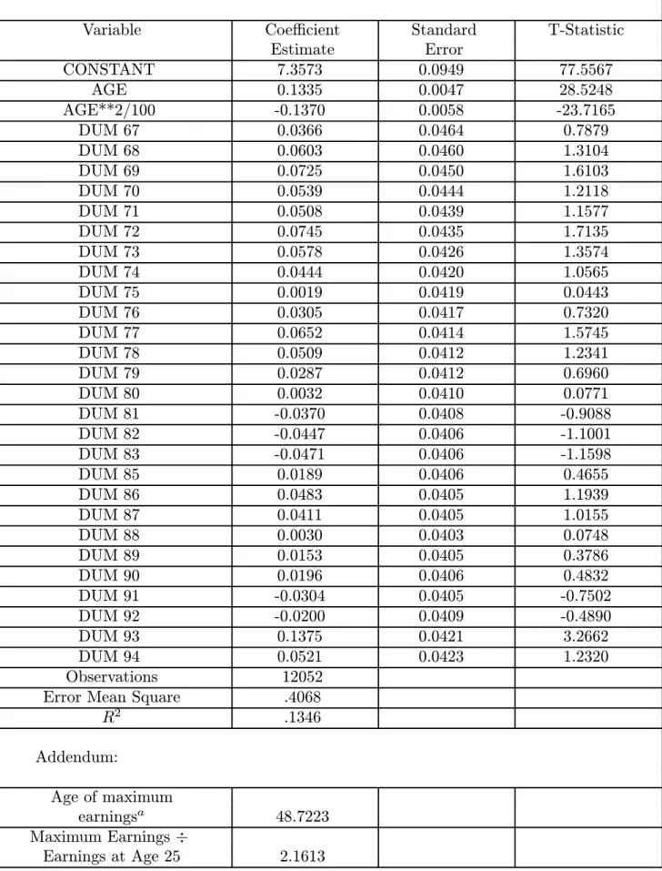
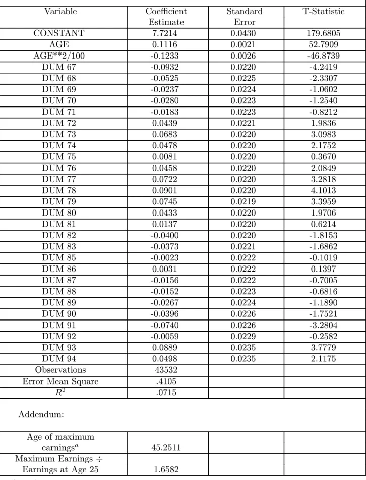
The estimates in Table A1 conform with our anticipations. Omitting the influence of technological progress, earnings peak in the age range 45—49.3 If we compare peak earnings with earnings at say age 25, the ratio is about 1.5 for the lowest education group and about 2.2 for the highest. Looking at the table for all education groups together, the time dummies show strong annual growth from technological change from 1967—1978; after that there is very little growth, and business cycle dips induce declines in the early 1980s and early 1990s. The slow growth in the second half of the period is consistent with the general slowdown in the rate of technological progress after the early 1970s, which economists have frequently noted.4
Table 2 is particularly important for this paper’s model: for individual ages, Table 2 presents weighted—average estimates of the variance of the residual from equation (1). The table omits the youngest workers – for whom labor market participation is especially erratic. Each column except the first then reveals a clear pattern: the variance of the regression error rises with age. The increase for thefirst column is miniscule. For column 2, however, between ages 25—39 and 46—60 the increase is 25%; for column 3, it is 62%; for college graduates, it is 65%; and for the sample as a whole, it is 44%.
Maximum Likelihood. As explained in the introduction, we assume that workers under-stand their initial earning differences but that young workers are unsure about how they will fair relative to their peers as the differences reshuffle and grow with age. The purpose of this paper is to study the consequences for saving behavior of the resulting uncertainty for individual households. The key to our analysis is the variance pattern in Table 2. To proceed, we examine the error term of equation (1) in detail.
A common approach in the earnings dynamics literature is to specify the regression error as the sum of two components:
it =µi+ηit, (2)
with µ an individual—specific characteristic, and η an independent, idiosyncratic error. This assumes that individuals have differences in life—long earning ability, which the life— long component of their regression error, µi, captures. Typically, one would assume that
3 Positive technological progress will increase the age at which earnings actually peak
– the faster the technological change, the later the peak.
4 It is also true that the PSID data on earnings corresponds to take home pay – it
omits “benefits” such as employer contributions to social security, to private pensions, and for medical insurance. To the extent that benefits have risen relative to wages and salaries in the recent past, the coefficients on the dummy variables are biased downward.
µ and η are independently normally distributed. This is the “random effects” model of . The random effects model by itself, however, will not explain the pattern of rising variances in Table 2.
Although one might guess that cross—sectional differences in earnings vary from year to year, that presumably does not lead to the variance pattern of Table 2. Earnings will tend to be high in general in years of business—cycle prosperity, and low in troughs, but our time dummies should capture such phenomena. Although conceivably cross—sectional variation is higher in some years than others, the PSID attempts to represent the entire population at each date: as the original respondents (from 1968) aged and died, the PSID replaced them with young households. Thus, the fraction of, say, 50 year olds in the sample should match the U.S. population as a whole in every year. Sample weights should correct for minor problems of representativeness, and all of our regressions use weights. Since the sample then represents all ages in every year, year to year cycles should not affect the pattern of variances by age in Table 2.
One possible hypothesis, say,H0, that could explain the pattern in Table 2 is that older
workers endure larger idiosyncratic shocks. In other words, perhaps the variance of ηit in (2) rises with age. For example, upward steps in earnings typically follow promotions, and for young workers promotions may be frequent and small, but for older workers promotions may be infrequent and sizable. Letting zit be the age of worker i at time t, a simple specification would then be
it =
µi+ηit, for zit ≤45,
µi+ηit∗, for zit >45, (3) where age 45 is the middle of a working life, µi and ηit and ηit∗ are independent normal random variables with zero mean, and the variance of η∗ is larger than the variance of η.
A second hypothesis, say, H00, is that µi changes over a worker’s life span. One story could be as follows. In youth, a worker does “technical” tasks – assembly line jobs, assigned research work, etc. In the second half of a career, a worker may rise to a managerial position in which he is directing younger workers. If a worker does assume managerial responsibilities, his earnings trajectory takes an upward step; if not, his earnings may be level or even erode as his technical skills become obsolete. Another story could be that some workers experience health problems in old age, and their earnings suffer, while others do not. A third possibility is that in youth, a worker trains for a career involving a particular technology or product; over time, the technology or product may grow in importance and the worker may prosper, or a new technology or product may arrive and make the worker’s training obsolete. A simple formulation is
it=
µi+ηit, for zit ≤45,
µ∗i +ηit, for zit >45, (4) where µ and µ∗ and η are normal random variables with zero means; η is independent of the other two; andµandµ∗ are distributed bivariate normal with the marginal distribution of the latter having a higher variance. We might expect the correlation coefficient for µ and µ∗ to be positive but less than one.
The procedure that we employ nests (3)—(4): we assume a components of error for-mulation
it= µµi∗+ηit, for zit ≤45,
i +ηit∗, for zit >45, (5) where µand µ∗ andη andη∗ are normal random variables with zero means; η andη∗ are each independent of the other three, and have varianceση andση∗, respectively; andµand µ∗ are distributed bivariate normal with marginal variances σµ and σµ∗ and correlation
ρ∈(−1,1).
Consider a household with index i. Let the vector θ includeαandβ from (1) and the variances and correlation from (5). Letting xit be the vector of covariates for household i at time t, use the notation
eit=e(yit, xit,θ)≡ln(yit)−α0−α1·zit −α2·[zit]2/100−
1994
j=1967
βj ·Dj(t). (6)
Let times before the household is age 45 be indexed with s; let the times after age 45 be indexed with t. Let the normal density function for a variable z with mean 0 and standard deviationσ beφ(z|σ). Then the likelihood function for the household if none of its observations are top coded is
Li(θ)≡ ∞ −∞ ∞ −∞ φ(µi, µ∗i |σµ,σµ∗,ρ)· s φ(eis−µi|ση)· t φ(eit−µ∗i |ση∗)dµidµ∗i . (7)
The likelihood function for top coded households is only slightly different. Top coding can only occur in 1983. Suppose household i is top coded at age ¯s < 45. Then the likelihood function for the household’s observations is
¯ Li(θ)≡ ∞ ei¯s ∞ −∞ ∞ −∞ φ(µi, µ∗i |σµ,σµ∗,ρ)·φ(e−µi|ση)· s φ(eis−µi|ση)· t φ(eit−µ∗i |ση∗)dµidµ∗i de . (8)
Similarly if the top coding occurs after age 45.
IfI is the set of non-top coded households and ¯I the set of top coded households, then maximum likelihood estimation determines θ from
θ = arg max θ0 i∈I Li(θ0)· ¯i∈I¯ ¯ L¯i(θ0). (9)
Table 2A in the Appendix exhibits maximum likelihood estimates ofαandβ. Rather than force the changes to take place instantly, we exclude observations for ages 3 years before and after age 45. The results resemble those from OLS in Table A1. This is not surprising: other than top coded observations, OLS should provide consistent estimates.
Table 3 presents our estimates of the precisions hη = 1/ση, hη∗ = 1/ση∗, hµ = 1/σµ, and hµ∗ = 1/σµ∗ and of the correlation coefficient ρ. Under H0, sinceση <ση∗, we would have
hη > hη∗ but hµ ≈hµ∗; under H00, since σµ <σµ∗, we would have
hη ≈hη∗ but hµ > hµ∗.
Table 3 strongly favorsH00. In every column, hµ> hµ∗: in columns 1—5, respectively, hµ∗ is 82% as large as hµ, 76%, 77%, 48%, and 68% as large. In most cases hη and hη∗ are almost the same. The one anomaly is column 1, where hη∗ is 18% larger than hη –
and even then the inequality is in the opposite direction from what H0 predicts.
The next section assumes H00 and turns to a model of household saving.
2. Life Cycle Saving
This section lays out a traditional life cycle model emphasizing saving for retirement. Then it adds the precautionary saving that is this paper’s focus.
Saving for Retirement. We begin with a traditional life—cycle model emphasizing saving in youth and middle age and dissaving in old age (e.g., Modigliani [1986]).
Let the number of “equivalent adults” per household be ns. Let a household’s head constitute 1 “equivalent adult.” For a married household, let the spouse constitute ξS
additional equivalent adults. Although ξS might be 1, it could also be substantially less if there are scale economies to household size. If at agesthe household head has a spouse, set nS
s = 1; otherwise, set nSs = 0. Similarly, let nCs be the number of children in a household when the head’s age is s, and let ξC be the adult equivalency of each child. A recent literature (e.g., Banks et al. [1998], Bernheim et al. [2001], Hurd and Rohwedder [2003]) identifies an empirical drop in consumption at retirement; Laitner [2003] associates this with the increase in leisure time. Let ξR be the drop at retirement. Then if R is the age of retirement, let
ns = 1 +ξ S ·nS
s +ξC ·nCs , if s < R,
ξR·(1 +ξS·nsS), if s≥R. . (10)
We follow Tobin [1967], who suggests a utility—flow model ns·u(
cs ns
).
The idea is that a single—member household with consumption c1 and the same household at a different age withnequivalent adults and consumptioncn achieve the same per capita
current utilityflow whencn =n·c1, and that a household weightsu(.) withnbecause the
household values the per capita utility flows of all members equally.
This paper’s life—cycle maximization model is then as follows: for household i, born at t, and retiring at age R, we solve for consumption cits at each age s
max cits T 0 e−δ·s·qs·nis·u cits nis ds (11)
subject to: ∂aits
∂s =rs·aits+ψis·w·(1−τ)·e
g·(t+s)+SS
its−cits, ait0 = 0 =aitT ,
aits ≥0 all s ,
where δ is the subjective discount rate; equivalent adults, nis, come from (10); and, aits is the household’s net worth (e.g., net asset) position at age s. We assume that financial institutions do not allow borrowing without collateral; hence, the household’s net worth can never be negative. As is common in the literature, we assume u(.) is isoelastic:5
u(x) = xγ
γ , with γ <1 and γ = 0;
ln(x), otherwise. (12) The maximal life span is T years.
The household suppliesψis“effective hours” in the labor market per hour of work time; thus, if w·eg·(t+s), where g >0 is the rate of labor augmenting technological progress, is the economy wide average wage rate, the household’s pretax earnings are ψis·w·eg·(t+s) per hour at age s. We assume a proportional income tax with rate τ. Life spans are uncertain. Let qs be the probability of surviving through age s. To simplify, we average male and female survival rates and assume a husband and wife die together. Aftertax earnings at age s are
ψis·w·eg·(t+s)·(1−τ).
We assume that markets offer actuarially fair annuities and that all households take advantage of them. The underlying interest rate is r. At age s, an annuity pays
r− q˙s qs .
This exceeds r sinceqs is a declining function of s. The aftertax rate of return on savings is rs ≡ r− ˙ qs qs · (1−τ). (13)
5 This is the only additively separable case with homotheticity. The latter is virtually
Economists have long realized that Social Security benefits reduce households’ needs for life—cycle wealth. The termSSitsin the budget constraint of (11) reflects Social Security taxes in youth and benefits in old age. The Social Security tax is proportional up to a cap; benefits vary with lifetime earnings and a progressive structure of brackets. This paper assumes that over time the cap and the benefit brackets move proportionately to the level eg·t of technology, which preserves the homothetic structure of (11).
Precautionary Saving. This subsection modifies the framework above to incorporate un-certainty about lifetime earnings. Although in our framework markets provide securities (i.e., annuities) that protect a household against mortality risk, we assume that prob-lems stemming from moral hazard preclude market insurance against earnings uncertainty. Households respond with self—insurance efforts. We call the additional wealth that self— insurance stimulates “precautionary saving.”
The earnings dynamics analysis of Section 1 provides the template. Each household’s age—trajectory of “effective hours” is a quadratic function of age:
Q(age)≡α0+α1·age +α2·
age2
100 , (14)
with αi as estimated – see Table A2 in the Appendix. Each household is born with a different earning ability – which Section 1’s individual effect µ captures. We assume that a household discovers its µ as it begins work. Nevertheless, in midlife the house-hold’s individual effect changes to µ∗, and we assume that though the household knows the distribution from which µ∗ will emerge, it only learns its actual realization from the distribution at age 45. Section 1 posits a bivariate normal distribution for (µ, µ∗) pairs in the population as a whole, with zero means and parametersσµ,σµ∗, andρ. For consistency with the regression model, we assume that condition on its beginning individual effect µ, a young household perceives that it faces a normal distribution for µ∗ with6
µ∗ ∼N ρ·(σµ∗/σµ)·µ, σ2µ∗ ·(1−ρ2) . (15) If Q(.) is as in (14) and household i is age s, and if M is midlife (M = 45 in this paper), we then have ψis ≡ψ(µi, µ∗i, s) = µi·Q(s), if s≤M, µ∗i ·Q(s), if M < s≤R, 0, if s > R, (16)
where R is the age of retirement. This paper treats R as exogenously given.7 From this point forward, we ignore the error componentsηandη∗ from our likelihood function: think of them as characterizing measurement error. Section 1 provides a possible story for the change from µi to µ∗i in midlife.
6 The first argument inN(., .) below is the mean, and the second is the variance. Note
that the mean in this case is the mean conditional on individual effectµin the first period of life; the unconditional mean, as stated, is zero by assumption.
Aggregate Household Life—Cycle Net Worth. Let At be aggregate household life—cycle net worth at time t if households face lifetime earning uncertainty, and let Act be the same in the certainty case.
Although our focus is precautionary saving, we develop a control, or comparison case as follows. Suppose household i, born at t, learns its µi and its µ∗i at its inception. Such households have no lifetime uncertainty; hence, they have no need for precautionary wealth accumulation. In this case, given (16), we can solve (11).8 Call the resulting net worth at
age s for a household born at time s and having earning abilities µ and µ∗ ac(µ, µ∗, t, s).
Let Section 1’s bivariate normal density for (µ, µ∗) be
φ(µ, µ∗|σµ,σµ∗,ρ),
recalling that the population means for µ and for µ∗ are zero. Then average household assets at time t are
T 0 ∞ −∞ ∞ −∞ φ(µ, µ∗|σµ,σµ∗,ρ)·qs·ac(µ, µ∗, t−s, s)dµ dµ∗ds . (17) Similarly, average gross—of—tax earnings are
w·eg·t· R 0 ∞ −∞ ∞ −∞ φ(µ, µ∗|σµ,σµ∗,ρ)·qs·ψ(µ, µ∗, s)·eg·sdµ dµ∗ds . (18) Call the integral in (18) E. If we multiply (17) by the population of the economy, we have Act; if we multiply (18) by the population, we have the economy’s gross—of—tax wage bill. A ratio of the two is independent of the population’s absolute size. Furthermore, an important consequence of homothetic preferences is that technological change and the wage w each affect (17) and (18) strictly proportionately. Thus,
Act
w·eg·t·E = Ac0
w·E , (19)
with the ratio independent of t, w, and the population.9
If there is lifetime earning uncertainty, the analysis is slightly more complicated. As before, let M be the age at midlife. Let J(aM, µ, µ∗, t) be second—period—of—life utility for a household born at t, entering its second period with net worth aM, having second— period—of—life earning ability µ∗, and having first—period ability µ. Then
8 Problem (11) is a standard optimal control problem – except for the constraint
aits ≥ 0. All of this paper’s computations employ Mariger’s [1987] algorithm for dealing with the constraint.
9 To be more precise, the fact that ratio (19) is independent of time and w reflects
the homotheticity of preferences, our assumptions about the Social Security system, and our assumptions that the underlying interest rate is fixed and the wage grows only with technology. The last assumptions mean that we are studying the household sector of an economy that has reached a so-called steady—state equilibrium.
J(aM, µ, µ∗, t)≡max cts T M e−δ·s·qs·ns·u cts ns ds (20) subject to: ∂ats ∂s =rs·ats+ψ(µ, µ ∗, s)·w·(1−τ)·eg·(t+s)+SS(µ, µ∗) ts−cts, atM =aM atT = 0, ats ≥0 alls ∈[M, T].
(Notice that J(.) depends on µ because a household’s Social Security benefits depend on its lifetime earnings – though ψ(µ, µ∗, s) for s ≥M does not dependent on µ.) Similarly, letI(aM, µ, t) be first—period—of—life utility if the household has earning abilityµand ends its first period with net worth aM. Since Social Security taxes depend only on current earnings, we can write SS(µ, .)ts fors ≤M. Then
I(aM, µ, t)≡max cts M 0 e−δ·s·qs·ns·u cts ns ds (21) subject to: ∂ats ∂s =rs·ats+ψ(µ, µ ∗, s)·w·(1−τ)·eg·(t+s)+SS(µ, .)ts −cts, at0 = 0 atM =aM, ats ≥0 all s∈[0, M]. For a given µ and t, we can solve for aM from
aM =aM(µ, t) = arg max
a {I(a, µ, t) +Eµ∗|µ J(a, µ, µ
∗, t) }, (22) where the density for µ∗ conditional on µcomes from (15).
For the model with uncertainty, our procedure is as follows: determineaM from (22); then determine assets a(µ, µ∗, t−s, s) from (20)—(21); and, then substitute the latter into (17) in place of ac(.). Line (18) remains as before. As in (19), our isoelastic preferences enable us to derive
At
w·eg·t·E = A0
w·E , (23)
with E as above, and with the last ratio independent of time, w, and the economy’s population.
3. Simulations
We want to compare (19) and (23) tofind the quantitative importance of precautionary saving. Laitner [2001] suggests the empirical ratio for 1995 of private net worth to gross— of—tax labor earnings for the U.S. was about 4.61.10 Because this paper’s model omits
estate building, we do not necessarily expect our simulations to produce ratios as high as the empirical one.
Calibration. Although early life—cycle analyses calibrated their parameters in part on the basis of author introspection (e.g., Tobin [1967]), this paper relies heavily on recent estimates from empirical studies.
The child, spouse, and retirement adult—equivalency weights in (10) are potentially important determinants of life—cycle saving – high relative weights for children, for exam-ple, front load household consumption and can drastically reduce total life—cycle wealth accumulation (e.g., Auerbach and Kotlikoff [1987, ch.11]). Many authors set ξC in the range of .30—.50 and ξS equal to 1.00 (e.g., Mariger [1987]). Using U.S. Consumer Expen-diture Survey data from 1984—2000, Laitner [2003] finds support for values ξS ≤ .50 and
ξC ≤.25. These presumably reflect returns to scale for larger households. In fact,ξS =.50 would be consistent with U.S. Social Security benefits to couples, and a low ξC perhaps implies that parents reduce their own consumption in years in which they have children at home. For our base case, we set ξS =.50 and ξC = .25. Banks et al. [1998], Bernheim et al. [2001], and Laitner [2003] find a consumption reduction of 10—20% or more upon retirement. For our base case, we set ξR =.85.
Typical values of the household subjective discount rateδare .00—.02, reflecting house-holds’ impatience to consumer sooner rather than later. Laitner [2003] finds that a house-hold’s consumption per capita seems to grow on average about 2%/year with age. With this rate of growth, a household’s consumption is roughly 2.2 times as high at age 65 as at age 25. Our simulations assume such a growth rate, and derive theδ in each case consistent with it.
The isoelastic parameterγ determines households’ degree of risk aversion: ifγ is near 1, utility is almost linear and households are quite comfortable with substantial year—to— year consumption unevenness; if γ is small, very negative in particular, utility is sharply concave and households are very averse to consumption fluctuations, hence they are very risk averse. Estimates in the literature range from γ = 0 to -4. For instance, Auerbach and Kotlikoff [1987] useγ =−3, Cooley and Prescott [1995] use 0, Rust and Phelan [1997] estimate -.072.11 On the basis of the size of the consumption decline at retirement,
Lait-ner [2003] estimates γ =−1 to -1.5.
We use a standard mortality table for 1995, averaging mortality rates for men and
10 Thefigure is based mainly on U.S. Flow of Funds data. Private net worth does include
the capitalized value of private pension rights, but it does not include Social Security benefits (which receive separate treatment in our analysis). The denominator of the ratio is GDP times labor’s share. Labor’s share is .7015 (which we determine from wages and salaries as a share of corporate output).
women. The average life expectancy is 77 years. For simplicity, we assume that a husband and wife die together.
For earnings, we use our estimates for the whole PSID sample ofαi from Table A2 in the Appendix. Our base—case estimates of hµ, hµ∗, and ρ are described in Section 1 and presented in column 5 of Table 3.
We use the U.S. Social Security System 1995 proportional tax rate, .1052, on earnings; the System’s earnings cap ($61,200/year for 1995); and its 1995 benefit formula. U.S. National Income and Product Account government spending (Federal and state and local) on goods and services suggestsτ =.231. Based on the slow rate of technological progress after 1970, we set g=.01.
For our base case, we set r = .05. This is derived as follows. The ratio of ratio of corporate wages and salaries to corporate output is about .2985.12 Multiplying this times GDP and subtracting total depreciation, we have return to capital net of depreciation. We further subtract the cost to households of financial services (e.g., brokerage fees and financial counseling, service charges of financial intermediaries, and handling expenses for life insurance and pension plans).13 Then we divide by the sum of the current—cost nonresidential private capital stock, the residential private capital stock, the government fixed capital stock, and the stock of business inventories. The ratio is the average rate of return on capital; under marginal cost pricing and constant returns to scale, this is also the marginal return. The average return 1951—2001 is .055; the 1995 return is .051. Our net—of—tax return for households is r ·(1 −τ). Other calculations are, of course, possible. If we exclude residential housing services from GDP, exclude depreciation on residential housing from total depreciation, and omit the stock of residential housing from our denominator above, the average (gross of tax) rate of return is .081, and the 1995 value is .076. Conversely, Laitner and Stolyarov [2003] argue that intangible capital may be 50 percent as large as the nonresidential capital stock, and with such a correction the average rate of return (reinstating residential capital) falls to .050 and the 1995 rate to .046.
There is no need to set w – homotheticity makes the numerators of (19) and (23) linear in w just as the denominator is, so the wage cancels out of the ratio in each case.
Table 4 summarizes our base—case parameter choices.
Simulations. Table 5 presents three sets of simulations. Thefirst, see row 1, generates ag-gregative ratiosA/(w·E) for our specification with uncertainty over earnings in the second half of life. A household resolves the uncertainty at age 45 – see (20)—(22). The second— row specification eliminates uncertainty,fixing, past age 45, mean earnings conditional on initial earnings. Economic theory shows that row 2 ratios will be smaller than row 1. The third row of Table 5 follows all possible first and second period of life outcomes, with a household knowing its µand µ∗ as it begins work – see (19). We take row 1 minus row 3 as our measure of precautionary wealth accumulation. (Note that there is no theoretical reason that this measure must always be positive.)
12 All of the U.S. National Income and Product Accounts data comes from
http://www.bea.doc.go/bea/nd1.ham,
either the interactive “NIPA tables” or the interactive “fixed asset tables.”
13 See lines 87—90 of interactive NIPA Table 2.4.5. In general, these “personal business
Table 5 presents results for values of γ between 0 and -4. As we would expect, a lowerγ, implying more curvature in the utility functionu(.), leads to higher precautionary wealth accumulation. For γ = 0, our measure of precautionary wealth, the difference between row 1 and row 3, is slightly negative. For γ =−1, precautionary saving increases national wealth by 5.3%; for γ = −1.5, the increase is 8.3%; for γ =−2, it is 11.1%; and, for γ = −4, the increase is 20.5%. Since the empirical ratio A/(w·E) is about 4.61, for
γ =−1 life—cycle saving including precautionary wealth accumulation explains about 73% of U.S. wealth. With γ =−2, the explained fraction rises to 77%; with γ =−4, it is 84%. For comparison, Modigliani [1986] argues that the life—cycle model can account for roughly 80% of U.S. net worth.
The last row of Table 5 suggests a problem with very low values ofγ: for γ less than -1, the corresponding value of the subjective discount rateδis negative – yet we explained above that values δ ∈ [0, .02], reflecting some impatience on the part of households, seem the most plausible. One possibility is that the empirical analysis yielding our base—case calibration of consumption growth did not include households’ uncertainty about their earnings – see, for example, Caballero [1990].
A second possibility is that slight changes in our calibrations would help. Mathemati-cally, if ˆct is the percentage growth rate of a household’s consumption per capita over ages in which the household’s composition is not changing and in which new information about future earnings is not becoming available, we have14
ˆ ct =
rt·(1−τ)−δ
1−γ . (24)
Our base case sets ˆct = .02. For a given γ, however, we can see that δ can be larger if rt is higher or if ˆct is lower. The lowest estimate of ˆct in Laitner [2003] is .0176. Table 6 considers .015 – a rate of growth at which a household’s consumption per capita would rise by a factor of about 1.8 over 40 years. If we exclude residential capital (and its service flow and depreciation), we argued above that we might set rt = .076. Table 6 considers this as well.
For either ˆct =.015 orrt =.076, Table 6 shows that a non-negativeδ emerges forγ as low as -1.5. Precautionary saving then augments life—cycle wealth accumulation by 6—7%. In both cases, the percent of U.S. net worth accounted for is smaller, however, than when
γ =−1 in Table 5.
A third possibility is that our utility function – although very standard in the eco-nomics literature – is too restrictive.15
We proceed assuming that values of γ much below -1 yield implausible implications forδ.
Returning to Table 5, the large difference between rows 2 and 3 is a surprise. Consider the column withγ =−1. In the certainty—equivalent case, each householdfinishes life with average earnings conditional on its starting earnings. Total life—cycle saving is only 58%
14 In fact, our numerical calculations assume discrete time – providing an approximation
to (24).
of empirical national net worth. In row 3, initial earnings are the same, but though there is a distribution of second—stage—of—life earnings, each household knows its second—stage realization as it begins adulthood.16 A household expecting a low second—period realization
will save extra in youth; a household expecting a high second—period realization will save less. The reactions will be asymmetric, however: the liquidity constraint ats ≥ 0 puts a restriction on the reduction in saving for a household anticipating high earnings late in life, but there is no corresponding limitation for the increase in saving for a household that is pessimistic about its future earnings. Row 3 generates 69—70% of empirical net worth. Making second—period—of—life earnings uncertain until age 45 – see row 1 – only increases life—cycle net worth to 73% of the empirical total. Although a full recognition of the uninsurable earning uncertainty that households face is appealing from the point of view of realism, in practice the step from row 2 to row 3 is much larger than the step from row 3 to row 1.
Sensitivity Analysis. Table 7 considers alternative child and retirement weights. In all cases the subjective discount rate remains as in Table 5.
Suppose γ =−1. With ξC =.50, a value consistent with Mariger [1987] and others, the role of precautionary saving virtually disappears (uncertainty actually lowers aggrega-tive life—cycle net worth slightly). As we would expect, higher consumption for children substantially lowers the fraction of empirical net worth that the model can explain – from 73 percent in Table 5 to 60 percent in Table 7.
With ξC = .25 as in Table 5, changes in the fall in consumption at retirement have little effect on the role of precautionary saving – as in Table 5, precautionary wealth accumulation is about 5 percent of the life—cycle total. As one would expect, if the weight on retirement consumption is higher, young households save more and aggregative life—cycle net worth is higher. In Table 5, life—cycle saving explains 75 percent of 1995 empirical net worth when γ =−1; in Table 7 it explains 78 percent with ξR =.90, but only 69 percent with ξR=.80.
Table 8 summarizes our last experiment. It employshµ,hµ∗, andρfrom column 4 (i.e., college graduates) in Table 3. The second—period—of—life standard deviation is noticeably higher, and the correlation ρ lower, than for other education categories. The college educated group makes up about one—quarter of the whole sample (by sampling weight).
Precautionary saving increases life—cycle accumulation by 7.4% in column 2, Table 8 – up from 5.3% in the same column of Table 5. Perhaps more surprising,Ac/(w·E) for the certainty case is 12% larger than Table 5. Again, asymmetric responses to increases and decreases of second—period earnings seem quantitatively more important to total wealth accumulation than uncertainty about second—period—of—life earnings.
16 In row 1, at age 22 a household knows its µ and the conditional distribution for its
µ∗; the household learns its actual µ∗ at age 45. In row 2, at age 22 a household learns µ and µ∗, with the latter equaling its conditional mean from row 1. In row 3, at age 22 a household learns both µ and µ∗; µ∗ can take any of the values possible in row 1.
4. Conclusion
This paper studies the quantitative importance of precautionary wealth accumula-tion relative to life—cycle saving for retirement. The first section examines panel data on earnings from the PSID. We find that the cross—sectional variance of earnings within a cohort rises with age. Using a bivariate normal model of random effects, we find that second—period—of—life earnings are strongly positively correlated with initial earnings but indeed have a higher variance. The paper’s next section studies the consequences for life— cycle saving. It assumes that households know their youthful earning power as they enter the labor market but that they know only the conditional distribution of their second— period—of—life earnings. Only in midlife do they learn their actual second—period earning ability.
For our most plausible calibrations, precautionary saving only adds 5—6% to aggrega-tive life—cycle wealth accumulation. Nevertheless, our earnings model emerges as quite important: even if second—period—of—life earning changes are fully predictable from youth, so that precautionary saving (i.e., responsiveness to uncertainty) plays no role, the vari-ety of earning profiles that our bivariate normal model generates itself stimulates enough extra wealth accumulation to merit careful consideration. In the presence of liquidity constraints, predictions of rising earnings decrease youthful saving less than anticipations of falling earnings raise it. In the end, heterogeneity of earning profiles, even without uncertainty, tends to increase aggregative life—cycle wealth accumulation.
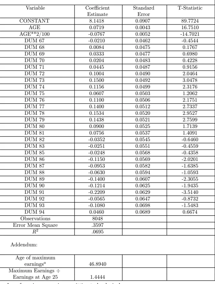
Table A1. Weighted Ordinary Least Squares PSID 1967—94: Less Than High School Education
Variable Coefficient Standard T-Statistic Estimate Error CONSTANT 8.1418 0.0907 89.7724 AGE 0.0719 0.0043 16.7510 AGE**2/100 -0.0767 0.0052 -14.7021 DUM 67 -0.0210 0.0462 -0.4544 DUM 68 0.0084 0.0475 0.1767 DUM 69 0.0333 0.0477 0.6980 DUM 70 0.0204 0.0483 0.4228 DUM 71 0.0445 0.0487 0.9156 DUM 72 0.1004 0.0490 2.0464 DUM 73 0.1500 0.0492 3.0478 DUM 74 0.1156 0.0499 2.3176 DUM 75 0.0607 0.0503 1.2062 DUM 76 0.1100 0.0506 2.1751 DUM 77 0.1400 0.0512 2.7337 DUM 78 0.1534 0.0520 2.9527 DUM 79 0.1438 0.0521 2.7599 DUM 80 0.0900 0.0525 1.7139 DUM 81 0.0756 0.0537 1.4091 DUM 82 -0.0352 0.0545 -0.6460 DUM 83 -0.0251 0.0551 -0.4559 DUM 85 -0.0248 0.0568 -0.4358 DUM 86 -0.1150 0.0569 -2.0201 DUM 87 -0.0953 0.0582 -1.6385 DUM 88 -0.0630 0.0594 -1.0593 DUM 89 -0.1400 0.0607 -2.3055 DUM 90 -0.1214 0.0625 -1.9435 DUM 91 -0.2209 0.0629 -3.5140 DUM 92 -0.0565 0.0647 -0.8732 DUM 93 -0.1080 0.0698 -1.5483 DUM 94 0.0460 0.0689 0.6674 Observations 8048 Error Mean Square .3597
R2 .0695 Addendum: Age of maximum earningsa 46.8940 Maximum Earnings ÷ Earnings at Age 25 1.4444
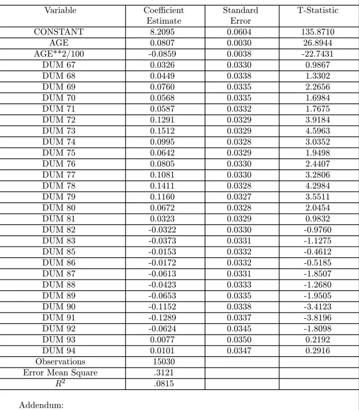
Table A1 (cont.). Weighted Ordinary Least Squares PSID 1967—94: High School Education
Variable Coefficient Standard T-Statistic Estimate Error CONSTANT 8.2095 0.0604 135.8710 AGE 0.0807 0.0030 26.8944 AGE**2/100 -0.0859 0.0038 -22.7431 DUM 67 0.0326 0.0330 0.9867 DUM 68 0.0449 0.0338 1.3302 DUM 69 0.0760 0.0335 2.2656 DUM 70 0.0568 0.0335 1.6984 DUM 71 0.0587 0.0332 1.7675 DUM 72 0.1291 0.0329 3.9184 DUM 73 0.1512 0.0329 4.5963 DUM 74 0.0995 0.0328 3.0352 DUM 75 0.0642 0.0329 1.9498 DUM 76 0.0805 0.0330 2.4407 DUM 77 0.1081 0.0330 3.2806 DUM 78 0.1411 0.0328 4.2984 DUM 79 0.1160 0.0327 3.5511 DUM 80 0.0672 0.0328 2.0454 DUM 81 0.0323 0.0329 0.9832 DUM 82 -0.0322 0.0330 -0.9760 DUM 83 -0.0373 0.0331 -1.1275 DUM 85 -0.0153 0.0332 -0.4612 DUM 86 -0.0172 0.0332 -0.5185 DUM 87 -0.0613 0.0331 -1.8507 DUM 88 -0.0423 0.0333 -1.2680 DUM 89 -0.0653 0.0335 -1.9505 DUM 90 -0.1152 0.0338 -3.4123 DUM 91 -0.1289 0.0337 -3.8196 DUM 92 -0.0624 0.0345 -1.8098 DUM 93 0.0077 0.0350 0.2192 DUM 94 0.0101 0.0347 0.2916 Observations 15030 Error Mean Square .3121
R2 .0815 Addendum: Age of maximum earningsa 46.9510 Maximum Earnings ÷ Earnings at Age 25 1.5127
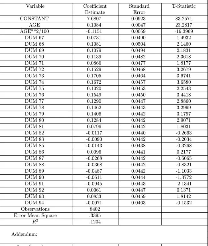
Table A1 (cont.). Weighted Ordinary Least Squares PSID 1967—94: Some College Education
Variable Coefficient Standard T-Statistic Estimate Error CONSTANT 7.6807 0.0923 83.2571 AGE 0.1084 0.0047 23.2817 AGE**2/100 -0.1151 0.0059 -19.3969 DUM 67 0.0731 0.0490 1.4932 DUM 68 0.1081 0.0504 2.1460 DUM 69 0.1079 0.0494 2.1831 DUM 70 0.1139 0.0482 2.3618 DUM 71 0.0866 0.0477 1.8177 DUM 72 0.1529 0.0468 3.2679 DUM 73 0.1705 0.0464 3.6741 DUM 74 0.1672 0.0457 3.6580 DUM 75 0.1020 0.0453 2.2543 DUM 76 0.1549 0.0450 3.4418 DUM 77 0.1290 0.0447 2.8860 DUM 78 0.1462 0.0443 3.2999 DUM 79 0.1406 0.0442 3.1797 DUM 80 0.1284 0.0442 2.9071 DUM 81 0.0796 0.0442 1.8031 DUM 82 -0.0117 0.0440 -0.2663 DUM 83 -0.0090 0.0442 -0.2034 DUM 85 -0.0143 0.0438 -0.3268 DUM 86 0.0096 0.0441 0.2177 DUM 87 -0.0268 0.0442 -0.6065 DUM 88 -0.0368 0.0442 -0.8321 DUM 89 -0.0487 0.0442 -1.1033 DUM 90 -0.0611 0.0444 -1.3772 DUM 91 -0.0945 0.0443 -2.1341 DUM 92 0.0061 0.0447 0.1371 DUM 93 0.0833 0.0459 1.8142 DUM 94 -0.0071 0.0463 -0.1532 Observations 8402 Error Mean Square .3395
R2 .1204 Addendum: Age of maximum earningsa 47.0866 Maximum Earnings ÷ Earnings at Age 25 1.7530
Table A1 (cont.). Weighted Ordinary Least Squares PSID 1967—94: College/more Education
Variable Coefficient Standard T-Statistic Estimate Error CONSTANT 7.3573 0.0949 77.5567 AGE 0.1335 0.0047 28.5248 AGE**2/100 -0.1370 0.0058 -23.7165 DUM 67 0.0366 0.0464 0.7879 DUM 68 0.0603 0.0460 1.3104 DUM 69 0.0725 0.0450 1.6103 DUM 70 0.0539 0.0444 1.2118 DUM 71 0.0508 0.0439 1.1577 DUM 72 0.0745 0.0435 1.7135 DUM 73 0.0578 0.0426 1.3574 DUM 74 0.0444 0.0420 1.0565 DUM 75 0.0019 0.0419 0.0443 DUM 76 0.0305 0.0417 0.7320 DUM 77 0.0652 0.0414 1.5745 DUM 78 0.0509 0.0412 1.2341 DUM 79 0.0287 0.0412 0.6960 DUM 80 0.0032 0.0410 0.0771 DUM 81 -0.0370 0.0408 -0.9088 DUM 82 -0.0447 0.0406 -1.1001 DUM 83 -0.0471 0.0406 -1.1598 DUM 85 0.0189 0.0406 0.4655 DUM 86 0.0483 0.0405 1.1939 DUM 87 0.0411 0.0405 1.0155 DUM 88 0.0030 0.0403 0.0748 DUM 89 0.0153 0.0405 0.3786 DUM 90 0.0196 0.0406 0.4832 DUM 91 -0.0304 0.0405 -0.7502 DUM 92 -0.0200 0.0409 -0.4890 DUM 93 0.1375 0.0421 3.2662 DUM 94 0.0521 0.0423 1.2320 Observations 12052 Error Mean Square .4068
R2 .1346 Addendum: Age of maximum earningsa 48.7223 Maximum Earnings ÷ Earnings at Age 25 2.1613
Table A1 (cont.). Weighted Ordinary Least Squares PSID 1967—94: All Education Groups
Variable Coefficient Standard T-Statistic Estimate Error CONSTANT 7.7214 0.0430 179.6805 AGE 0.1116 0.0021 52.7909 AGE**2/100 -0.1233 0.0026 -46.8739 DUM 67 -0.0932 0.0220 -4.2419 DUM 68 -0.0525 0.0225 -2.3307 DUM 69 -0.0237 0.0224 -1.0602 DUM 70 -0.0280 0.0223 -1.2540 DUM 71 -0.0183 0.0223 -0.8212 DUM 72 0.0439 0.0221 1.9836 DUM 73 0.0683 0.0220 3.0983 DUM 74 0.0478 0.0220 2.1752 DUM 75 0.0081 0.0220 0.3670 DUM 76 0.0458 0.0220 2.0849 DUM 77 0.0722 0.0220 3.2818 DUM 78 0.0901 0.0220 4.1013 DUM 79 0.0745 0.0219 3.3959 DUM 80 0.0433 0.0220 1.9706 DUM 81 0.0137 0.0220 0.6214 DUM 82 -0.0400 0.0220 -1.8153 DUM 83 -0.0373 0.0221 -1.6862 DUM 85 -0.0023 0.0222 -0.1019 DUM 86 0.0031 0.0222 0.1397 DUM 87 -0.0156 0.0222 -0.7005 DUM 88 -0.0152 0.0223 -0.6816 DUM 89 -0.0267 0.0224 -1.1890 DUM 90 -0.0396 0.0226 -1.7521 DUM 91 -0.0740 0.0226 -3.2804 DUM 92 -0.0059 0.0229 -0.2582 DUM 93 0.0889 0.0235 3.7779 DUM 94 0.0498 0.0235 2.1175 Observations 43532 Error Mean Square .4105
R2 .0715 Addendum: Age of maximum earningsa 45.2511 Maximum Earnings ÷ Earnings at Age 25 1.6582
Table A2. Weighted Maximum Likelihood PSID 1967—94: Less Than High School Education
Variable Coefficient Standard T-Statistic Estimate Error CONSTANT 8.279941 0.096553 85.7553 AGE 0.066201 0.004187 15.8112 AGE**2/100 -0.072579 0.004948 -14.6690 DUM 67 -0.007690 0.037809 -0.2034 DUM 68 0.000855 0.038217 0.0224 DUM 69 0.041521 0.037923 1.0949 DUM 70 0.016641 0.037884 0.4393 DUM 71 0.014586 0.037706 0.3868 DUM 72 0.088604 0.037620 2.3552 DUM 73 0.125054 0.036977 3.3820 DUM 74 0.101226 0.037021 2.7343 DUM 75 0.028708 0.036697 0.7823 DUM 76 0.071199 0.036390 1.9566 DUM 77 0.069135 0.036201 1.9098 DUM 78 0.118541 0.036450 3.2521 DUM 79 0.098236 0.036104 2.7209 DUM 80 0.034143 0.036306 0.9404 DUM 81 0.025908 0.036723 0.7055 DUM 82 -0.073257 0.036943 -1.9830 DUM 83 -0.066577 0.037259 -1.7869 DUM 85 -0.058271 0.038735 -1.5043 DUM 86 -0.154304 0.039222 -3.9342 DUM 87 -0.084447 0.040748 -2.0724 DUM 88 -0.032542 0.042085 -0.7732 DUM 89 -0.067380 0.043294 -1.5563 DUM 90 -0.107726 0.045134 -2.3868 DUM 91 -0.199414 0.045936 -4.3411 DUM 92 -0.064014 0.047054 -1.3604 DUM 93 -0.056603 0.051189 -1.1058 DUM 94 0.065458 0.051374 1.2741 Observations 6680 -Log(likelihood) 4193.8052 Addendum: Age of maximum earningsa 45.6061 Maximum Earnings ÷ Earnings at Age 25 1.3609
Table A2 (cont.). Weighted Maximum Likelihood PSID 1967—94: High School Education
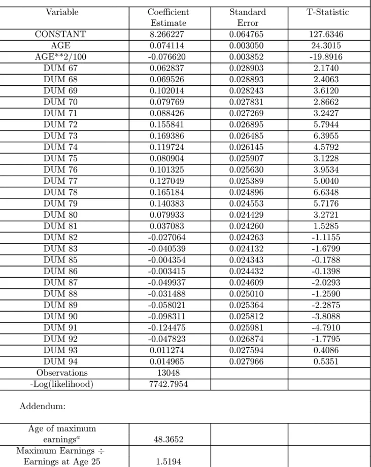
Variable Coefficient Standard T-Statistic Estimate Error CONSTANT 8.266227 0.064765 127.6346 AGE 0.074114 0.003050 24.3015 AGE**2/100 -0.076620 0.003852 -19.8916 DUM 67 0.062837 0.028903 2.1740 DUM 68 0.069526 0.028893 2.4063 DUM 69 0.102014 0.028243 3.6120 DUM 70 0.079769 0.027831 2.8662 DUM 71 0.088426 0.027269 3.2427 DUM 72 0.155841 0.026895 5.7944 DUM 73 0.169386 0.026485 6.3955 DUM 74 0.119724 0.026145 4.5792 DUM 75 0.080904 0.025907 3.1228 DUM 76 0.101325 0.025630 3.9534 DUM 77 0.127049 0.025389 5.0040 DUM 78 0.165184 0.024896 6.6348 DUM 79 0.140383 0.024553 5.7176 DUM 80 0.079933 0.024429 3.2721 DUM 81 0.037083 0.024260 1.5285 DUM 82 -0.027064 0.024263 -1.1155 DUM 83 -0.040539 0.024132 -1.6799 DUM 85 -0.004354 0.024343 -0.1788 DUM 86 -0.003415 0.024432 -0.1398 DUM 87 -0.049937 0.024609 -2.0293 DUM 88 -0.031488 0.025010 -1.2590 DUM 89 -0.058021 0.025364 -2.2875 DUM 90 -0.098311 0.025812 -3.8088 DUM 91 -0.124475 0.025981 -4.7910 DUM 92 -0.047823 0.026874 -1.7795 DUM 93 0.011274 0.027594 0.4086 DUM 94 0.014965 0.027966 0.5351 Observations 13048 -Log(likelihood) 7742.7954 Addendum: Age of maximum earningsa 48.3652 Maximum Earnings ÷ Earnings at Age 25 1.5194
Table A2 (cont.). Weighted Maximum Likelihood PSID 1967—94: Some College Education
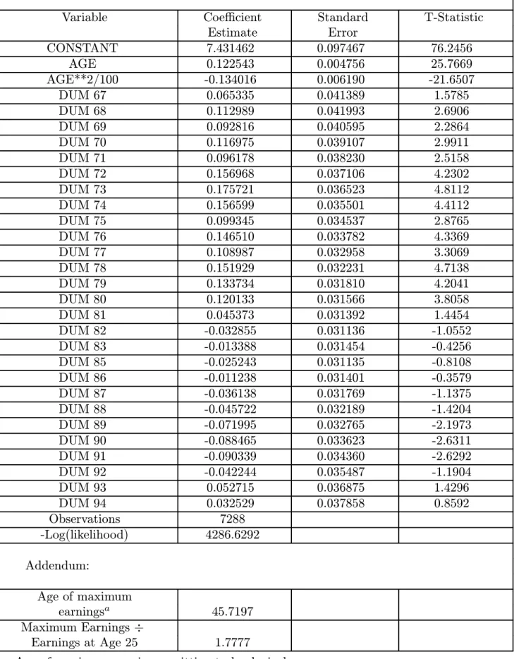
Variable Coefficient Standard T-Statistic Estimate Error CONSTANT 7.431462 0.097467 76.2456 AGE 0.122543 0.004756 25.7669 AGE**2/100 -0.134016 0.006190 -21.6507 DUM 67 0.065335 0.041389 1.5785 DUM 68 0.112989 0.041993 2.6906 DUM 69 0.092816 0.040595 2.2864 DUM 70 0.116975 0.039107 2.9911 DUM 71 0.096178 0.038230 2.5158 DUM 72 0.156968 0.037106 4.2302 DUM 73 0.175721 0.036523 4.8112 DUM 74 0.156599 0.035501 4.4112 DUM 75 0.099345 0.034537 2.8765 DUM 76 0.146510 0.033782 4.3369 DUM 77 0.108987 0.032958 3.3069 DUM 78 0.151929 0.032231 4.7138 DUM 79 0.133734 0.031810 4.2041 DUM 80 0.120133 0.031566 3.8058 DUM 81 0.045373 0.031392 1.4454 DUM 82 -0.032855 0.031136 -1.0552 DUM 83 -0.013388 0.031454 -0.4256 DUM 85 -0.025243 0.031135 -0.8108 DUM 86 -0.011238 0.031401 -0.3579 DUM 87 -0.036138 0.031769 -1.1375 DUM 88 -0.045722 0.032189 -1.4204 DUM 89 -0.071995 0.032765 -2.1973 DUM 90 -0.088465 0.033623 -2.6311 DUM 91 -0.090339 0.034360 -2.6292 DUM 92 -0.042244 0.035487 -1.1904 DUM 93 0.052715 0.036875 1.4296 DUM 94 0.032529 0.037858 0.8592 Observations 7288 -Log(likelihood) 4286.6292 Addendum: Age of maximum earningsa 45.7197 Maximum Earnings ÷ Earnings at Age 25 1.7777
Table A2 (cont.). Weighted Maximum Likelihood PSID 1967—94: College/more Education
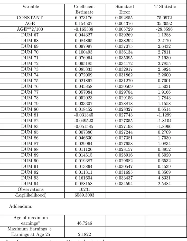
Variable Coefficient Standard T-Statistic Estimate Error CONSTANT 6.973176 0.092855 75.0972 AGE 0.154507 0.004376 35.3092 AGE**2/100 -0.165338 0.005729 -28.8596 DUM 67 0.044327 0.039269 1.1288 DUM 68 0.084895 0.038292 2.2170 DUM 69 0.097997 0.037075 2.6432 DUM 70 0.100493 0.036134 2.7811 DUM 71 0.076964 0.035095 2.1930 DUM 72 0.095185 0.034172 2.7855 DUM 73 0.085333 0.032917 2.5924 DUM 74 0.072009 0.031862 2.2600 DUM 75 0.021892 0.031270 0.7001 DUM 76 0.045858 0.030509 1.5031 DUM 77 0.057084 0.029784 1.9166 DUM 78 0.052023 0.029156 1.7843 DUM 79 0.033307 0.028818 1.1558 DUM 80 0.018452 0.028327 0.6514 DUM 81 -0.031345 0.027743 -1.1299 DUM 82 -0.049523 0.027355 -1.8104 DUM 83 -0.051585 0.027198 -1.8966 DUM 85 0.007380 0.027244 0.2709 DUM 86 0.046630 0.027381 1.7030 DUM 87 0.029964 0.027658 1.0834 DUM 88 0.011126 0.028157 0.3952 DUM 89 0.014515 0.028916 0.5020 DUM 90 0.019387 0.029682 0.6532 DUM 91 0.013864 0.030547 0.4539 DUM 92 0.011311 0.031695 0.3569 DUM 93 0.161604 0.033437 4.8331 DUM 94 0.088158 0.034594 2.5484 Observations 10231 -Log(likelihood) 6589.3093 Addendum: Age of maximum earningsa 46.7246 Maximum Earnings ÷ Earnings at Age 25 2.1822
Table A2 (cont.). Weighted Maximum Likelihood PSID 1967—94: All Education Groups
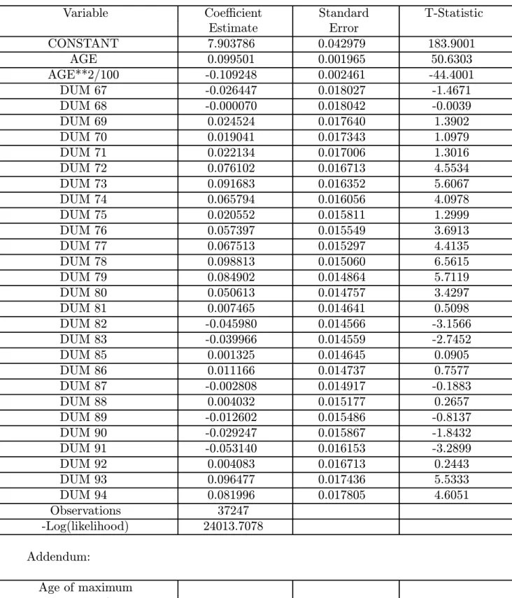
Variable Coefficient Standard T-Statistic Estimate Error CONSTANT 7.903786 0.042979 183.9001 AGE 0.099501 0.001965 50.6303 AGE**2/100 -0.109248 0.002461 -44.4001 DUM 67 -0.026447 0.018027 -1.4671 DUM 68 -0.000070 0.018042 -0.0039 DUM 69 0.024524 0.017640 1.3902 DUM 70 0.019041 0.017343 1.0979 DUM 71 0.022134 0.017006 1.3016 DUM 72 0.076102 0.016713 4.5534 DUM 73 0.091683 0.016352 5.6067 DUM 74 0.065794 0.016056 4.0978 DUM 75 0.020552 0.015811 1.2999 DUM 76 0.057397 0.015549 3.6913 DUM 77 0.067513 0.015297 4.4135 DUM 78 0.098813 0.015060 6.5615 DUM 79 0.084902 0.014864 5.7119 DUM 80 0.050613 0.014757 3.4297 DUM 81 0.007465 0.014641 0.5098 DUM 82 -0.045980 0.014566 -3.1566 DUM 83 -0.039966 0.014559 -2.7452 DUM 85 0.001325 0.014645 0.0905 DUM 86 0.011166 0.014737 0.7577 DUM 87 -0.002808 0.014917 -0.1883 DUM 88 0.004032 0.015177 0.2657 DUM 89 -0.012602 0.015486 -0.8137 DUM 90 -0.029247 0.015867 -1.8432 DUM 91 -0.053140 0.016153 -3.2899 DUM 92 0.004083 0.016713 0.2443 DUM 93 0.096477 0.017436 5.5333 DUM 94 0.081996 0.017805 4.6051 Observations 37247 -Log(likelihood) 24013.7078 Addendum: Age of maximum earningsa 45.5391 Maximum Earnings ÷ Earnings at Age 25 1.5854
Bibliography
[1] Abowd, John; and, Card, David, “On the Covariance Structure of Earnings and Hours Changes,” Econometrica 57, no. 2 (March 1989): 411—446.
[2] Aiyagari, S.R., “Uninsured Idiosyncratic Risk and Aggregate Saving,”Quarterly Jour-nal of Economics 109, no. 2 (May 1994): 659—684.
[3] Altig, David; Auerbach, Alan J.; Kotlikoff, Laurence J.; Smetters, Kent A.; and Walliser, Jan, “Simulating Fundamental Tax Reform in the United States,” American Economic Review vol. 91, no. 3 (June 2001): 574—595.
[4] Auerbach, Alan J.; and Kotlikoff, Laurence J. Dynamic Fiscal Policy. Cambridge: Cambridge University Press, 1987.
[5] Banks, James; Blundell, Richard; and Tanner, Sarah, “Is There a Retirement—Savings Puzzle?” American Economic Review 88, no. 4 (September 1998): 769—788.
[6] Barro, Robert J., “Are Government Bonds Net Worth?” Journal of Political Economy 82, no. 6 (November/December 1974): 1095—1117.
[7] Barsky, Robert; Kimball, Miles; Juster, F. Thomas; and Shapiro, Matthew, “Pref-erence Parameters and Behavioral Heterogeneity: An Experimental Approach in the Health and Retirement Study,” Quarterly Journal of Economics vol. 112, no. 2 (May 1997): 537—579.
[8] Bernheim, B. Douglas, Skinner, Jonathan, and Weinberg, Steven, “What Accounts for the Variation in Retirement Wealth Among U.S. Households,” American Economic Review 91, no. 4 (September 2001): 832—857.
[9] Caballero, Ricardo J., “Consumption Puzzles and Precautionary Savings,”Journal of Monetary Economics 25, no. 1 (January 1990): 113—136.
[10] Cooley, Thomas F., and Prescott, Edward C., “Economic Growth and Business Cy-cles,” in T.F. Cooley, ed., Frontiers of Business Cycle Research. Princeton, New Jersey: Princeton University Press, 1995.
[11] Deaton, A., “Saving and Liquidity Constraints,” Econometrica 59, no. 5 (September 1991): 1221—1248.
[12] Gokhale, Jagadeesh; Kotlikoff, Laurence J.; Sefton, James; and Weale, Martin, “Sim-ulating the Transmission of Wealth Inequality via Bequests,” Journal of Public Eco-nomics vol. 79, no. ‘ (January 2001): 93—128.
[13] Hurd, Michael; and Rohwedder, Susann, “The Retirement—Consumption Puzzle: An-ticipated and Actual Declines in Spending at Retirement,” NBER working paper 9586, http://www.nber.org/papers/w9586.
[14] Laitner, John, “Wealth Accumulation in the U.S.: Do Inheritances and Bequests Play a Significant Role?” Michigan Retirement Research Center working paper 2001—019, www.mrrc.isr.umich.edu, 2001.
[15] Laitner, John, “Wealth Inequality and Altruistic Bequests,” American Economic Re-view vol. 92, no. 2 (May 2002): 270—273.
[16] Laitner, John, “Labor Supply Responses to Social Security,” Michigan Retirement Research Center working paper 2003—050, www.mrrc.isr.umich.edu, 2003.
[17] Laitner, John, “Wealth Accumulation in the U.S.: Do Inheritances and Bequests Play a Significant Role?” working paper, Department of Economics, University of Michigan, February, 2004.
[18] Laitner, John; and, Stolyarov, Dmitriy, “Technological Change and the Stock Mar-ket,” American Economic Review 93, no. 4 (September 2003): 1240—1267.
[19] Lillard, Lee; and, Weiss, Yoram. “Components of Variation in Panel Earnings Date: American Scientists 1960—70,” Econometrica 47, no. 2 (March 1979): 54—77.
[20] Mariger, Randall P., “A Life—Cycle Consumption Model with Liquidity Constraints: Theory and Empirical Results,” Econometrica 55, no. 3 (May 1987): 533—557.
[21] Modigliani, Franco, “Life Cycle, Individual Thrift, and the Wealth of Nations,” Amer-ican Economic Review76, no. 3 (June 1986): 297—313.
[22] Rust, John; and, Phelan, Christopher. “How Social Security and Medicare Affect Retirement Behavior in a World of Incomplete Markets,” Econometrica 65, no. 4 (July 1997): 781—831.
[23] Tobin, J., “Life Cycle Saving and Balanced Growth,” in W. Fellner (ed.), Ten Eco-nomic Studies in the Tradition of Irving Fisher. New York: Wiley, 1967.
[24] Weil, Philippe, “Nonexpected Utility in Macroeconomics,”Quarterly Journal of Eco-nomics 105, no. 1 (February 1990): 29—42.
[25] Zeldes, Stephen, “Optimal Consumption with Stochastic Income: Deviations from Certainty Equivalence,” Quarterly Journal of Economics104, no. 2 (May 1989): 275— 298.
Table 1. Panel Study of Income Dynamics Sample 1967—1994a
Panel less high some college all
Length: than school college or
HS more 1—5 329 278 103 108 818 6—10 161 214 104 99 578 11—15 114 184 87 129 514 16—20 99 165 95 130 489 21—25 63 175 102 167 507 26—28 47 121 79 114 361 Total House— holds: 813 1137 570 747 3267 Total Obs. 8,048 15,030 8,402 12,052 43,532 Obs. with Censured Earnings 1 4 4 59 68 Obs. with Adjusted Hours:b 1,594 2,155 1,164 1,609 6,522 Obs. Dropped Zero Hrs: 98 122 107 117 444 Average Earningsc $19,264 $23,954 $27,076 $38,723 $27,778
a. Men only; no poverty sample; ages max{education+ 6,16} to 60. b. Work hours adjusted upward to minimum 1750 hours/year. c. Arithmetic average; 1984 dollars; NIPA consumption deflator.
Table 2. Estimated Variance of Residual from Weighted OLS: PSID Sample 1967—1994a
Age less high some college all
than school college or
HS more 25 0.311984 0.398072 0.212237 0.300392 0.329970 26 0.262474 0.354262 0.254899 0.264066 0.313142 27 0.260435 0.210086 0.290596 0.258597 0.266634 28 0.395252 0.194260 0.281459 0.245593 0.282218 29 0.260636 0.207678 0.217061 0.315352 0.277497 30 0.365447 0.266462 0.341118 0.279861 0.335799 31 0.431972 0.290941 0.267845 0.260505 0.327952 32 0.215023 0.293851 0.277570 0.274925 0.311889 33 0.274406 0.324884 0.271092 0.288077 0.332506 34 0.385872 0.248387 0.290102 0.295364 0.346200 35 0.379533 0.279906 0.286025 0.393355 0.388124 36 0.400243 0.269780 0.335601 0.305611 0.373906 37 0.446240 0.243054 0.250060 0.341668 0.369742 38 0.446234 0.340350 0.286133 0.386692 0.416816 39 0.295150 0.318533 0.254221 0.534404 0.434403 40 0.267611 0.292404 0.299539 0.395925 0.387590 41 0.306671 0.308220 0.246820 0.420451 0.392671 42 0.316903 0.278106 0.261265 0.340663 0.363474 43 0.280287 0.260034 0.239901 0.571841 0.413591 44 0.259459 0.263336 0.419063 0.440348 0.409213 45 0.318383 0.258221 0.400519 0.788129 0.519896 46 0.311886 0.246555 0.348500 0.319797 0.380750 47 0.274505 0.327321 1.054556 0.415975 0.538985 48 0.297978 0.248192 0.536444 0.368542 0.411322 49 0.326165 0.313183 0.269459 0.875103 0.525585 50 0.313074 0.306346 0.325590 0.421587 0.418631 51 0.327585 0.344874 0.292986 0.413396 0.425698 52 0.347307 0.380379 0.411005 0.383428 0.456921 53 0.276323 0.301929 0.416874 0.489554 0.436239 54 0.353970 0.433464 0.355427 0.441288 0.475476 55 0.312131 0.463306 0.417202 0.508088 0.508746 56 0.353727 0.367588 0.392770 0.654748 0.505648 57 0.440915 0.424415 0.331049 0.649548 0.558536 58 0.402615 0.387770 0.404991 0.557092 0.522803 59 0.372167 0.387991 0.513761 0.728239 0.551823
Table 2 (cont.). Estimated Variance of Residual from Weighted OLS: PSID Sample 1967—1994a
Aver— less high some college all
age than school college or
for HS more
Age
25—39 0.342060 0.282701 0.274401 0.316297 0.340453
46—60 0.351944 0.352180 0.443121 0.530550 0.489763
a. As in Table 1: men only; no poverty sample; ages max{education+ 6,16} to 60; work hours adjusted upward to minimum 1750 hours/year.
Table 3. Maximum Likelihood Precision Estimates (Standard Deviation): PSID Sample 1967—1994a
Para— less high some college all
meter than school college or
HS more hµ 2.3882 2.6407 2.6428 2.4991 2.2968 (0.0963) (0.0707) (0.0947) (0.0762) (0.0359) hη 2.4195 2.5894 2.6326 2.4747 2.4952 (0.0300) (0.0191) (0.0246) (0.0201) (0.0109) hµ∗ 1.9724 2.0141 2.0213 1.1856 1.5614 (0.0690) (0.0751) (0.1260) (0.0573) (0.0324) hη∗ 2.8461 2.6717 2.4546 2.4879 2.6286 (0.0383) (0.0349) (0.0526) (0.0412) (0.0202) ρ 0.7955 0.7165 0.6471 0.5749 0.7009 (0.0405) (0.0390) (0.0671) (0.0530) (0.0217) a. As in Table 1: men only; no poverty sample; ages max{education+ 6,16} to 60; work hours
Table 4. Parameter Values and Empirical Ratios
Name Value
Parameter
ξC .25
ξS .50
ξR .85
consumption growth with age .02
τ .231
g .01
Social Security tax rate .1052
r .05 hµ 2.2968 hµ∗ 1.5614 ρ .7009 Age adulthood 22 child bearing 24 M 45 retirement 64 T 90 Ratio
aggregate net worth/labor earnings 4.610 Source: see text.
Table 5. Simulation Results: Ratio wA
·E for Base—Case Calibration
γ = 0 γ =−1 γ =−1.5 γ =−2 γ =−4 Uncertainty Case 3.167 3.380 3.475 3.564 3.868 Certainty—equivalent Case 2.679 2.679 2.679 2.679 2.679 Certainty Case 3.209 3.209 3.209 3.209 3.209
[Row 1 - Row 3] ÷ Row 3
-.013 .053 .083 .111 .205
Uncertainty—CaseA/(w·E) ÷ empirical ratio
.687 .733 .754 .773 .839
Implied Subjective Discount Rate δ
.018 -.002 -.012 -.022 -.063
Table 6. Simulation Results: Ratio wA
·E for Alternative Calibrations
γ = 0 γ =−1 γ =−1.5 γ =−2 γ =−4 Calibration with ˆct =.015 Uncertainty Case 2.514 2.704 2.791 2.873 3.152 Certainty—equivalent Case 2.057 2.057 2.057 2.057 2.057 Certainty Case 2.633 2.633 2.633 2.633 2.633
[Row 1 - Row 3] ÷Row 3
-.045 .027 .060 .091 .197
Uncertainty—CaseA/(w·E) ÷ empirical ratio
.545 .587 .605 .623 .684
Implied Subjective Discount Rate δ
.023 .008 .001 -.007 -.037 Calibration with rt =.076 Uncertainty Case 2.804 3.021 3.117 3.208 3.510 Certainty—equivalent Case 2.306 2.306 2.306 2.306 2.306 Certainty Case 2.909 2.909 2.909 2.909 2.909
[Row 1 - Row 3] ÷Row 3
-.036 .039 .072 .103 .207
Uncertainty—CaseA/(w·E) ÷ empirical ratio
.608 655 .676 .696 .761
Implied Subjective Discount Rate δ
.037 .018 .008 -.002 -.042
Table 7. Simulation Results: Ratio wA
·E for Alternative Values of ξC and ξR
γ = 0 γ =−1 γ =−1.5 γ =−2 γ =−4 Calibration with ξC =.50 Uncertainty Case 2.562 2.768 2.863 2.952 3.257 Certainty Case 2.795 2.795 2.795 2.795 2.795
[Row 1 - Row 2] ÷ Row 2
-.083 -.010 .024 .056 .165
Uncertainty—CaseA/(w·E) ÷ empirical ratio
.556 .600 .621 .640 .707 Calibration with ξR =.80 Uncertainty Case 2.961 3.171 3.265 3.353 3.652 Certainty Case 3.019 3.019 3.019 3.019 3.019
[Row 1 - Row 2] ÷ Row 2
-.019 .050 .081 .111 .210
Uncertainty—CaseA/(w·E) ÷ empirical ratio
.642 .688 .708 .727 .792 Calibration with ξR =.90 Uncertainty Case 3.370 3.585 3.682 3.772 4.087 Certainty Case 3.397 3.397 3.397 3.397 3.397
[Row 1 - Row 2] ÷ Row 2
-.008 .055 .084 .110 .203
Uncertainty—CaseA/(w·E) ÷ empirical ratio
.731 .778 .799 .818 .887
Table 8. Simulation Results: Ratio wA
·E for Table 3, column 4, Precisions and Correlation Coefficient
γ = 0 γ =−1 γ =−1.5 γ =−2 γ =−4 Uncertainty Case 3.520 3.871 4.017 4.153 4.587 Certainty—equivalent Case 2.445 2.445 2.445 2.445 2.445 Certainty Case 3.604 3.604 3.604 3.604 3.604
[Row 1 - Row 3] ÷ Row 3
-.023 .074 .115 .152 .273
Uncertainty—Case A/(w·E) ÷ empirical ratio
.763 .840 .871 .901 .995
Implied Subjective Discount Rateδ
.018 -.002 -.012 -.022 -.063