Sur les methodes efficaces d’estimation statistique a haute dimension

(1)

HAL Id: tel-02433016

https://hal.archives-ouvertes.fr/tel-02433016

Submitted on 8 Jan 2020

HAL is a multi-disciplinary open access archive for the deposit and dissemination of sci-entific research documents, whether they are pub-lished or not. The documents may come from

L’archive ouverte pluridisciplinaire HAL, est destinée au dépôt et à la diffusion de documents scientifiques de niveau recherche, publiés ou non, émanant des établissements d’enseignement et de

On Efficient Methods for High-dimensional Statistical

Estimation

Dmitry Babichev

To cite this version:

Dmitry Babichev. On Efficient Methods for High-dimensional Statistical Estimation. Machine Learn-ing [stat.ML]. PSL Research University, 2019. English. �tel-02433016�

(2)

TH `ESE DE DOCTORAT

de l’Universit´e de recherche Paris Sciences Lettres

PSL Research University

Préparée à l’ École normale supérieure

On Efficient Methods for High-dimensional Statistical Estimation

Sur les m´ethodes efficaces d’estimation statistique `a haute dimension

´Ecole doctorale n

◦

386

´ECOLE DOCTORALE DE SCIENCES MATH ´EMATIQUES DE PARIS CENTRE

Sp´ecialit´e

INFORMATIQUE

COMPOSITION DU JURY:

M. Arnak Dalalyan

ENSAE ParisTech, Rapporteur M. St´ephane Chr´etien

NPL, Rapporteur M. Francis Bach

Inria Paris, Directeur de th`ese M. Anatoli Juditsky

UGA, Co-directeur de th`ese Olivier Capp´e

CNRS, Pr´esident du Jury Franck Iutzeler

UGA, Membre du Jury

Soutenue par Dmitry Babichev le 22.02.2019

Dirig´ee parFrancis BACH

(3)

(4)

The best angle from which to approach any problem is the try-angle

(5)

(6)

Abstract

In this thesis we consider several aspects of parameter estimation for statistics and machine learning, and optimization techniques applicable to these problems. The goal of parameter estimation is to find the unknown hidden parameters, which govern the data, for example parameters of an unknown probability density. The construction of estimators through optimization problems is only one side of the coin, finding the optimal value of the parameter often is an optimization problem that needs to be solved, using various optimization techniques. Hopefully these optimization problems are convex for a wide class of problems, and we can exploit their structure to get fast convergence rates.

The first main contribution of the thesis is to develop moment-matching techniques for multi-index non-linear regression problems. We consider the classical non-linear regression problem, which is unfeasible in high dimensions due to the curse of di-mensionality; that is why we assume a model, which states that in fact the data is a nonlinear function of several linear projections of data. We combine two existing techniques: average derivative estimator (ADE) and Sliced Inverse Regression (SIR) to develop the hybrid method (SADE) without some of the weak sides of its parents: it works both in multi-index models and with weak assumptions on the data distri-bution. We also extend this method to high-order moments. We provide theoretical analysis of constructed estimators both for finite sample and population cases.

In the second main contribution we use a special type of averaging for stochastic gradient descent. We consider generalized linear models for conditional exponential families (such as logistic regression), where the goal is to find the unknown value of the parameter. Classical approaches, such as Stochastic Gradient Descent (SGD) with constant step-size are known to converge only to some neighborhood of the optimal value of the parameter, even with Rupert-Polyak averaging. We propose the averaging of moment parameters, which we call prediction functions. For finite-dimensional models this type of averaging surprisingly can lead to negative error, i.e., this approach provides us with the estimator better than any linear estimator can ever achieve. For infinite-dimensional models our approach converges to the optimal prediction, while parameter averaging never does.

The third main contribution of this thesis deals with Fenchel-Young losses. We consider multi-class linear classifiers with the losses of a certain type, such that their

(7)

dual conjugate has a direct product of simplices as a support. The corresponding saddle-point convex-concave formulation has a special form with a bilinear matrix term and classical approaches suffer from the time-consuming multiplication of ma-trices. We show, that for multi-class SVM losses, under mild regularity assumption and with smart matrix-multiplication sampling techniques, our approach has an iter-ation complexity which is sublinear in the size of the data. It means, that to do one iteration, we need to pay only trice 𝑂(𝑛+𝑑+𝑘): for number of classes 𝑘, number

of features 𝑑 and number of samples 𝑛, whereas all existing techniques use at least

one of 𝑛𝑑, 𝑛𝑘 or𝑑𝑘 arithmetical operations per iteration. This is possible due to the

right choice of geometries and using a mirror descent approach.

Keywords : parameter estimation, moment-matching, constant step-size SGD, conditional exponential family, Fenchel-Young loss, mirror descent.

(8)

Résumé

Dans cette thèse, nous examinons plusieurs aspects de l’estimation des paramètres pour les statistiques et les techniques d’apprentissage automatique, aussi que les méthodes d’optimisation applicables à ces problèmes. Le but de l’estimation des paramètres est de trouver les paramètres cachés inconnus qui régissent les données, par exemple les paramètres dont la densité de probabilité est inconnue. La construction d’estimateurs par le biais de problèmes d’optimisation n’est qu’une partie du prob-lème, trouver la valeur optimale du paramètre est souvent un problème d’optimisation qui doit être résolu, en utilisant diverses techniques. Ces problèmes d’optimisation sont souvent convexes pour une large classe de problèmes, et nous pouvons exploiter leur structure pour obtenir des taux de convergence rapides.

La première contribution principale de la thèse est de développer des techniques d’appariement de moments pour des problèmes de régression non linéaire multi-index. Nous considérons le problème classique de régression non linéaire, qui est irréalisable dans des dimensions élevées en raison de la malédiction de la dimensionnalité et c’est pourquoi nous supposons que les données sont en fait une fonction non linéaire de plusieurs projections linéaires des données. Nous combinons deux techniques exis-tantes : “average derivative estimator” (ADE) et “Sliced Inverse Regression” (SIR) pour développer la méthode hybride (SADE) sans certains des aspects faibles de ses parents : elle fonctionne à la fois dans des modèles multi-index et avec des hypothèses faibles sur la distribution des données. Nous étendons également cette méthode aux moments d’ordre élevé. Nous fournissons une analyse théorique des estimateurs con-struits à la fois pour les cas d’échantillons finis et les cas population.

Dans la deuxième contribution principale, nous utilisons un type particulier de calcul de la moyenne pour la descente stochastique du gradient. Nous considérons des modèles linéaires généralisés pour les familles exponentielles conditionnelles (comme la régression logistique), où l’objectif est de trouver la valeur inconnue du paramètre. Les approches classiques, telles que la descente à gradient stochastique (SGD) avec une taille de pas constante, ne convergent que vers un certain voisinage de la valeur optimale du paramètre, même avec le calcul de la moyenne de Rupert-Polyak. Nous proposons le calcul de la moyenne des paramètres de moments, que nous appelons fonctions de prédiction. Dans le cas des modèles à dimensions finies, ce type de calcul de la moyenne peut, de façon surprenante, conduire à une erreur négative, c’est-à-dire que cette approche nous fournit un estimateur meilleur que tout estimateur linéaire ne

(9)

peut jamais le faire. Pour les modèles à dimensions infinies, notre approche converge vers la prédiction optimale, alors que le calcul de la moyenne des paramètres ne le fait jamais.

La troisième contribution principale de cette thèse porte sur les pertes de Fenchel-Young. Nous considérons des classificateurs linéaires multi-classes avec les pertes d’un certain type, de sorte que leur double conjugué a un produit direct de simplices comme support. La formulation convexe-concave à point-selle correspondante a une forme spéciale avec un terme de matrice bilinéaire, et les approches classiques souffrent de la multiplication des matrices qui prend beaucoup de temps. Nous montrons que pour les pertes SVM multi-classes, sous hypothèse de régularité légère et avec des techniques d’échantillonnage efficaces, notre approche a une complexité d’itération qui est sous-linéaire dans la taille des données. Cela signifie que pour faire une itération, nous n’avons besoin de payer que trois fois : 𝑂(𝑛+𝑑+𝑘) pour le nombre de classes 𝑘,

le nombre de caractéristiques 𝑑 et le nombre d’échantillons 𝑛, alors que toutes les

techniques existantes utilisent au moins une des opérations arithmétiques 𝑛𝑑, 𝑛𝑘 ou 𝑑𝑘 par itération. Ceci est possible grâce au bon choix des géométries et à l’utilisation

d’une approche de descente en miroir.

Mots Clés : estimation des paramètres, méthode des moments, SGD à pas con-stant, famille exponentielle conditionnelle, fonction objectif du Fenchel-Young, de-scente en miroir.

(10)

Acknowledgements

First of all, I would like to thank my supervisor Francis Bach. His guidance and ability to explain difficult concepts in easy words is the quality, which helped me through all my Ph.D. His politics of open door, when anyone can come and answer questions when his door is open was a great support. Also, I would like to thank my co-advisor Anatoli Juditsky, with whom I had several very fruitful discussions and who instilled in me statistical thinking.

This thesis has received funding from the European Union’s H2020 Framework Programme (H2020-MSCA-ITN-2014) under grant agreement n642685 MacSeNet. I would like to thank Helen Cooper for all the training, summer schools and workshops she helped to organize as a part of this framework. I am grateful to Pierre Van-dergheynst, with whom I had an opportunity to work during my academic internship in Lausanne, EPFL. I am also grateful to Dave Betts, who was my mentor to the audio restoration field during my industrial internship in Cambridge.

I also would like to thank Arnak Dalalyan and Stephane Chretien for accepting to review my thesis. I would also like to express my sincere gratitude to Olivier Cappé and Franck Iutzeler for accepting to be part of the jury for my thesis.

I would like to thank all members of Willow and Sierra team, old and new ones, for all the group meetings, thanks to which I expanded my scientific outlook. Especially I want to say thank you to my friend and colleague Dmitrii Ostrovskii, with whom I was working on the 3rd project, and who was able to explain me a large amount of information in a short time.

Also, I am grateful to all my friends with whom I spent a lot of joyful hours and days and who share my hobbies. I would like to thank Andrey, Dasha, Kolya, Tolik, Anya and Katya, my teammates in the intellectual game "What? Where? When?". I would like to thank Marwa, who introduced me to the world of climbing. Thank you, Vitalic for our almost daily talks. Also, I say thank my friends Denis, Dima, and Petr for their support.

I would like to thank my parents who opened for me a wonderful world of math-ematics and their faith in me. I say thank my sister Tanka for all her sister care and readiness to come to the rescue at any moment.

Last but not least, I am very grateful to my girlfriend Tatiana Shpakova for her love and who was always there in easy and difficult times.

(11)

(12)

Contributions and thesis outline

In Chapter 1 we give a brief overview of parameter estimation, concerning the

method of moments, maximum likelihood and loss minimization problems.

Chapter2is dedicated to a special application of method of moments for non-linear regression. This chapter is based on the journal article: Slice inverse regression with score functions, D. Babichev, F. Bach, In Electronic Journal of Statistics [Babichev and Bach, 2018b]. The main contributions of this chapter are as follows:

— We propose score function extensions to sliced inverse regression problems, both for the first-order and second-order score functions.

— We consider the infinite sample case and show that in the population case our estimators are superior to the non-sliced versions.

— We consider also finite sample case and show their consistency given the exact score functions. We provide non-asymptotical bounds, given sub-Gaussian assumptions.

— We propose to learn the score function as well, in two steps, i.e., first learning the score function and then learning the effective dimension reduction space, or directly, by solving a convex optimization problem regularized by the nuclear norm.

— We illustrate our results on a series of experiments.

In Chapter 3we consider special type of averaging for Stochastic SGD applied to generalized linear models. This chapter is based on the conference paper published as an UAI 2018 paper, which was accepted as an oral presentation: Constant step size stochastic gradient descent for probabilistic modeling, D. Babichev, F.Bach, Proceed-ings in Uncertainty in Artificial Intelligence [Babichev and Bach, 2018a]. The main contributions of this chapter are:

— For generalized linear models, we propose averaging moment parameters in-stead of natural parameters for constant step size stochastic gradient descent. — For finite-dimensional models, we show that this can sometimes (and

supris-ingly) lead to better predictions than the best linear model.

— For infinite-dimensional models, we show that it always converges to optimal predictions, while averaging natural parameter never does.

(17)

benchmarks with many observations.

In Chapter 4 we develop sublinear method for Fenchel-Young losses, this is joint work with Dmitrii Ostrovskii. We have submitted this work to ICML 2019 under a title Sublinear-time training of mlticlass classifiers with Fenchel-Young losses, Dmitry Babichev, Dmitrii Ostrovskii and Francis Bach. The main contributions of this chap-ter are:

— We develop efficient algorithms for solving the regularized empirical risk min-imization problems via associated saddle-point problem and using : (i) sam-pling for computationally heavy matrix multiplication and (ii) right choice of geometry for mirror descent type algorithms.

— The less aggressive partial sampling scheme is applicable for any loss mini-mization problem, such that its dual conjugate has a direct product of simlices as a support. This leads to the cost 𝑂(𝑛(𝑑+𝑘)) of one iteration.

— The more aggressive full sampling scheme, applied to multiclass hinge loss leads to the sublinear cost 𝑂(𝑑+𝑛+𝑘) of one iteration.

(18)

Chapter 1

Introduction

In this chapter we give the brief overview of two main pillars of this thesis: param-eter estimation, and optimization (mostly convex minimization and convex-concave saddle point problems).

1.1 Principles for parameter estimation

Parameter estimation is a branch of statistics and machine learning, that solves problems of estimation of an unknown set of parameters given some observations. There are a big variety of different methods and models and we consider the three probably most famous of them: moment matching, maximum likelihood and risk min-imization. The main application of parameter estimation is density and conditional density estimation (and more generally model estimation), which in turn are used in regression, classification and clustering problems.

1.1.1 Moment matching

Moment matching is a technique for finding the values of parameters, using sev-eral moments of the distribution, i.e., expectations of powers of random variable. The method of moments was introduced at least by Chebyshev and Pearson in the late 1800s (see for example [Casella and Berger, 2002] for a discussion). Suppose, that we have a real valued random variable 𝑋 drawn from a family of distributions

{𝑓(_{· |}𝜃)_|𝜃_∈Θ_}.

Given a sample (𝑥1, . . . , 𝑥𝑛), the goal is to estimate the true value of the

parame-ter 𝜃*. The classical approach is to consider the first𝑘 moments: 𝜇𝑖 =E[𝑋𝑖] =𝑔𝑖(𝜃),

𝑖= 1, . . . , 𝑘, and solve the non-linear system of equations to find the estimator 𝜃ˆ: ⎧ ⎪ ⎪ ⎪ ⎪ ⎨ ⎪ ⎪ ⎪ ⎪ ⎩ ˆ 𝜇1 = 1 𝑛 𝑛 ∑︀ 𝑖=1 𝑥𝑖 =𝑔1(ˆ𝜃), ... ˆ 𝜇𝑘 = 1 𝑛 𝑛 ∑︀ 𝑖=1 𝑥𝑘 𝑖 =𝑔𝑘(ˆ𝜃).

(19)

Even though the method is called moment matching, it is non necessary to use moments of random variable, but in general it can use any functions ℎ𝑖(𝑋) as long

as the expectations ∫︀

ℎ𝑖(𝑥)𝑓(𝑥|𝜃)𝑑𝑥 can be easily computed. This approach can be

extended for the case of random vectors and cross-moments [Hansen,1982]. Now we discuss some good and bad points of this approach. Also we illustrate the method on several examples, starting from the toy ones and finishing with state-of-the-art methods applicable to non-linear regression.

Disadvantages and advantages

The main advantage of this approach is that it is quite simple and the estimators are consistent under mild assumptions [Hansen, 1982]. Also in some cases the solu-tions can be found in closed form, where maximum likelihood approach may require a large computational effort.

However in some sense, this approach is inferior to the maximum likelihood ap-proach and estimators are often biased. In some cases, especially for small samples, the results can be outside of the parameter space. Also the nonlinear set of equations may be hard to solve.

Uniform distribution example

Let us start with a simple example, where we need to estimate the parameters of the one-dimensional uniform distribution: 𝑋 _∼ 𝑈[𝑎, 𝑏]. The first and the second moments can be evaluated as𝜇1 =E𝑋 = ₂1(𝑎+𝑏) and 𝜇2 =E𝑋2 = 1₃(𝑎2 +𝑎𝑏+𝑏2). Solving the system of these two equations, given a sample (𝑥1, . . . , 𝑥𝑛) and using the

sample moments 𝜇ˆ1 and 𝜇ˆ2 instead of true ones, we get a formula for estimating parameters 𝑎 and 𝑏: (𝑎, 𝑏) = (ˆ𝜇1− √︁ 3(ˆ𝜇2−𝜇ˆ21),𝜇ˆ1+ √︁ 3(ˆ𝜇2−𝜇ˆ21)). Linear regression example

Consider now a simple linear regression model, where 𝑦=𝑥⊤𝑏+𝜀, where 𝑦 _∈_R,

vectors 𝑥, 𝑏 _∈ _R𝑑 and error _𝜀 has a zero expectation. The goal is to estimate the

unknown vector of parameters 𝑏. Consider the cross moment _E(𝑥𝑖𝑦) =_E(𝑥𝑖𝑥⊤𝑏), for 𝑖 = 1, . . . , 𝑑, where 𝑥𝑖 _{is the} _𝑖_{-th component of} _𝑥_{. Replacing the expectations with}

empirical ones for the sample (𝑥𝑖, 𝑦𝑖), we get the equation:

𝑦1𝑥1+· · ·+𝑦𝑛𝑥𝑛 𝑛 = 𝑥1𝑥⊤1 +· · ·+𝑥𝑛𝑥⊤𝑛 𝑛 · ˆ 𝑏,

which is the traditional normal equation [Goldberger, 1964]. Finally, arranging the vectors in the matrix 𝑋 _∈ _R𝑛×𝑑 and 𝑦 _∈ _R𝑛, we recover the ˆ𝑏 = (𝑋𝑇𝑋)−1𝑋𝑇𝑦,

Hence in this particular formulation the moment matching estimator coincides with the ordinary least squares estimator.

(20)

Exponential families

Note, that for exponential families with probability density given by 𝑓(𝑥_|𝜃) = ℎ(𝑥) exp(𝜃⊤𝑇(𝑥)₋𝐴(𝜃), moment matching is equivalent to maximum likelihood es-timation [Lehmann and Casella, 2006]. We discuss this in more details in the next section.

Score functions

Consider the general non-linear regression problem

𝑦=𝑓(𝑥) +𝜀, 𝑥_∈_R𝑑, 𝑦 _∈_R, error 𝜀 independent of the data and _E𝜀= 0.

The ambitious goal is to estimate the unknown function 𝑓, given samples (𝑥𝑖, 𝑦𝑖).

However it is impossible to solve this problem in this loose formulation, due to the curse of dimensionality and parametric regression setup. Indeed, classical non-parametric estimation results show that convergence rates with any relevant perfor-mance measure can decrease as 𝑛−𝐶/𝑑 [Tsybakov, 2009, Györfi et al., 2002]. This

means that the number of sample points 𝑛 to reach some level of precision is

expo-nential in the dimension𝑑. A classical way to circumvent the curse of dimensionality

is to impose an additional condition: the dependence on some hidden lower dimension of data. Let us start with a simple assumption:

— 𝑥 is normal and 𝑓(𝑥) = 𝑔(𝑤⊤𝑥), with a matrix𝑤_∈_R𝑑×𝑘_.

If 𝑘 = 1, this model is called a single-index model and a multi-index in the other case [Horowitz,2012]. In this formulation, the goal is to estimate the unknown matrix of parameters𝑤_∈_R𝑘×𝑑 and we can use moment matching techniques. We use again

cross-moments and it is not difficult to show that for a single-index, using Stein’s lemma, that E(𝑦𝑥)∼ 𝑤1 [Stein, 1981, Brillinger, 1982]. Indeed, using independence of noise, the Gaussian probability density 𝑝(𝑥) _∼ exp(₋𝑥2_/₂₎ and integration by parts: E(𝑦𝑥) =E(︀(𝑓(𝑥) +𝜀)𝑥)︀ =E(︀𝑔(𝑤⊤1𝑥)𝑥 )︀ = ∫︁ 𝑔(𝑤⊤₁𝑥)𝑝(𝑥)𝑥𝑑𝑥= = ∫︁ 𝑔(𝑤⊤₁𝑥)_∇𝑝(𝑥)𝑑𝑥= ∫︁ ∇𝑔(𝑤₁⊤𝑥)𝑝(𝑥)𝑑𝑥_∼𝑤1.

The straightforward extension of this approach uses the notion of score function:

𝒮1(𝑥) =−∇log𝑝(𝑥),

where𝑝(𝑥)is the probability density of data𝑥. We use a moment matching technique

in the form E(𝒮1(𝑥)𝑦)∼𝑤1 as it is done in [Stoker,1986]. The most recent approach for multi-index models by [Janzamin et al., 2014] and [Janzamin et al., 2015] uses the notion of high-order scores 𝒮𝑚(𝑥) = (−1)𝑚

∇(𝑚)_𝑝₍_𝑥₎

𝑝(𝑥) (which are tensors) and cross moments E[𝑦· 𝒮𝑚(𝑥)] to train neural networks.

(21)

Contribution of this thesis

One more extension of the method of moments uses conditional moments E(𝑥|𝑦),

known as Sliced Inverse Regression (SIR, [Li, 1991]) and second order moments

E(𝑥𝑥⊤|𝑦) (Principal Hessian Directions PHD, [Li, 1992]) which use a normal

dis-tribution assumption. We develop a new method, combining strong sides of Stein’s

lemma and SIR in Chapter2of this thesis. We proposed new approaches (SADE and

SPHD) and develop analysis for both population and sample cases.

1.1.2 Maximum likelihood

Maximum likelihood estimation or MLE is an another classical approach to es-timate the unknown parameters, maximizing the likelihood function: it means intu-itively, that the selected parameter makes the data most probable. More formally, let

𝑋 = (𝑥1, . . . , 𝑥𝑛)be a random sample from a family of distributions{𝑓(· |𝜃)|𝜃 ∈Θ},

then

ˆ

𝜃 _∈arg max

𝜃∈Θ ℒ

(𝜃;𝑋),

where ℒ(𝜃;𝑋) = 𝑓𝑋(𝑋|𝜃) is the so-called Likelihood function: that is, the joint

probability density for the given realization of sample.

In practice, it is often convenient to work with the negative natural logarithm of the likelihood function, called the negative log-likelihood: 𝑙(𝜃;𝑋) =₋ln_ℒ(𝜃;𝑋). If the data (𝑥1, . . . , 𝑥𝑛) are independent and identically distributed, then the joint

distribution density can be written as a product of densities for a single 𝑥𝑖 and the

average negative log-likelihood minimization problem takes the form: arg min 𝜃∈Θ ˆ 𝑙(𝜃;𝑋) = arg min 𝜃∈Θ − 1 𝑛 𝑛 ∑︁ 𝑖=1 ln𝑓(𝑥𝑖 |𝜃),

where 𝑓(𝑥𝑖|𝜃)is the value of the probability density at the point 𝑥𝑖.

Advantages and disadvantages

Under mild assumptions the maximum likelihood estimator is consistent, asymp-totically efficient and asympasymp-totically normal [LeCam, 1953, Akaike, 1998]. Even though for a simple model, solutions can be found in closed form, for more advanced models, methods of optimization must be used to get the solution. Hopefully the optimization problem is convex for a wide class of likelihood estimators, such as ex-ponential families and conditional exex-ponential families [Koller and Friedman, 2009,

Murphy, 2012]. On the other hand, the optimization problem could be not convex if we consider for example mixture models. Moreover, maximum likelihood estimators are robust to mis-specified data: if the real data distribution 𝑓* does not come from

the model {𝑓(_{· |}𝜃) _| 𝜃 _∈ Θ_}, we can still use the approach and the solution with infinity data will be the projection (in the Kullback-Leibler sense) of 𝑓* to the set of

(22)

Example: Exponential families

The probability density for an exponential family can be written in the following form:

𝑓(𝑥_|𝜃) =ℎ(𝑥) exp(𝜃⊤𝑇(𝑥)₋𝐴(𝜃)),

where ℎ(𝑥) is the base measure, 𝑇(𝑥) _∈_R𝑑 is the sufficient statistics and 𝐴 the

log-partition function, which is always convex. Note that we do not assume that the data distribution𝑝(𝑥)comes from this exponential family. Then the average negative log-likelihood is equal to ˆ ℓ(𝜃;𝑥) = 1 𝑛 𝑛 ∑︁ 𝑖=1 [︁ 𝐴(𝜃)₋𝜃⊤𝑇(𝑥𝑖) ]︁ ,

which is a convex problem and can be solved, using any convex minimization ap-proach. Another view to this problem is moment matching: the solution can be found as: 𝐴′(𝜃) = 1 𝑛 𝑛 ∑︁ 𝑖=1 𝑇(𝑥𝑖),

where we consider the moment of the sufficient statistics 𝑇(𝑥). Note, that in a fact a big variety of classical distributions can be represented in this form: Bernoulli, normal, Poisson, exponential, Gamma, Beta, Dirichlet and many others. However, also, there are few which are not for example Student’s distribution and mixtures of classical distribution are not in this family.

Example: Conditional Exponential families

Now, let us consider the classical conditional exponential families:

𝑓(𝑦_|𝑥, 𝜃) = ℎ(𝑦)_·exp(𝑦_·𝜂𝜃(𝑥)−𝑎(𝜂𝜃(𝑥))).

Again, writing down the average negative log-likelihood, the goal is to minimize 1 𝑛 𝑛 ∑︁ 𝑖=1 [︁ −𝑦𝑖·𝜂𝜃(𝑥𝑖) +𝑎(𝜂𝜃(𝑥𝑖)) ]︁ .

These families are used for regression and classification problems and closely related to the generalized linear models [McCullagh and Nelder,1989], if the natural parameter is linear combination in known basis: 𝜂𝜃(𝑥) =𝜃⊤Φ(𝑥). On of the most popular choices

of function 𝑎′(_·)is the sigmoid function 𝑎′(𝑡) = 𝜎(𝑡) = 1/(1 +𝑒−𝑡), which leads to the logistic regression model. Let us illustrate the connection of logistic regression with a Bernoulli distribution. Let𝑝be a parameter of Bernoulli distribution with𝑥_{∈ {}0,1_}, then the probability density is written as:

𝑞(𝑥_|𝑝) =𝑥log𝑝₋(1₋𝑥) log(1₋𝑝) =𝑥log 𝑝

(23)

= exp(𝑥_·𝜃₋log(1 +𝑒𝜃)),

where𝜃 = log₁₋𝑝_𝑝 and hence logistic model is unconstrained reformulation of Bernoulli model, and the lack of constraint is often seen as a benefit for optimization.

Another common choice is Poisson regression [McCullagh, 1984], where 𝑎(𝑡) = exp(𝑡), which is used, when the dependent variable is a count.

Contribution of this thesis

In Chapter 3 of this thesis we consider constant step-size stochastic gradient de-scent for conditional exponential families. Instead of averaging of parameters 𝜃, we

propose averaging of so-called prediction functions 𝜇 = 𝑎′(𝜃⊤Φ(𝑥)), which leads to better convergence to the optimal prediction, especially for infinite-dimensional mod-els.

1.1.3 Loss functions

One more view to the parameter estimation problem is risk minimization, which goes beyond the maximum likelihood approach. A non-negative real-valued loss func-tion ℓ(𝑦,𝑦ˆ) measures the performance for classification or regression problem: i.e., the difference between prediction 𝑦ˆof a and the true outcome 𝑦. The expected loss 𝑅(𝜃) = _E[ℓ(𝑓(𝑥_|𝜃), 𝑦)] is called the risk. However, in practice the true distribution 𝑃(𝑥, 𝑦)is inaccessible and the empirical risk used instead. Hence, the classical regu-larized empirical risk minimization problem is written as:

min 𝜃 1 𝑛 𝑛 ∑︁ 𝑖=1 ℓ(︀𝑓(𝑥𝑖|𝜃), 𝑦𝑖 )︀ +𝜆Ω(𝜃), (1.1.1)

where Ω(𝜃) is a regularizer, which is used to avoid overfitting. There are several classical choices of loss function, and we start with in some sense the most intuitive ones:

0₋1 loss

This loss, which is also called misclassification loss is used in classification prob-lems, where the response 𝑦 is located in a finite set. The definition speaks for itself:

the loss is zero, in the case of true classification and one in the other case:

ℓ(𝑓(𝑥𝑖|𝜃), 𝑦𝑖) = 1 ⇐⇒ 𝑓(𝑥𝑖|𝜃)̸=𝑦𝑖.

It is known to lead to NP-hard problems, even for linear classifiers [Feldman et al.,

2012,Ben-David et al.,2003]. That is why in practice people use a convex relaxation of the 0₋1 loss functions (see below).

(24)

Quadratic loss

One of the other classical choices for loss function in the case of regression problems is the quadratic loss:

ℓ(𝑓(𝑥𝑖|𝜃), 𝑦𝑖) = (𝑓(𝑥𝑖|𝜃)−𝑦𝑖)2.

It has a simple form, smooth (in contradiction to the ℓ1 loss) and convex. Thus, the empirical risk minimization problem becomes mean squared error minimization.

The connection with likelihood estimators can be shown, using the linear model with Gaussian noise:

𝑦=𝑥⊤𝜃+𝜀, where 𝜀_{∼ 𝒩}(0, 𝜎2).

Then, the negative log-likelihood is

𝑙(𝑦;𝑥, 𝜃)_∼(𝑥⊤𝜃₋𝑦)2,

and the empirical likelihood minimization problem for this problem is equivalent to the mean squared error minimization (but the application of least squares is not limited to Gaussian noise).

Let us illustrate also a connection of quadratic loss with regression: consider that we are looking for a function 𝑓, such that 𝑦 = 𝑓(𝑥) +𝜀, where 𝑥 _∈ _R𝑑 _and _𝑦 _∈

R.

Then, the expected loss (risk) can be written as

𝑅(𝑓) = ∫︁

ℓ(𝑓(𝑥), 𝑦)𝑝(𝑥, 𝑦) 𝑑𝑥 𝑑𝑦.

Solving this functional minimization problem for the quadratic loss, we get the solu-tion 𝑓(𝑥) = _E𝑦[𝑦|𝑥], which is the conditional expectation of 𝑦 given 𝑥 and is known

as the regression function. Convex surrogates

Here we consider the main examples for convex surrogates of the 0₋1loss, which make the computation more tractable.

Hinge loss. It is written as

ℓ(𝑓(𝑥𝑖|𝜃), 𝑦𝑖) = max(0,1−𝑓(𝑥𝑖|𝜃)𝑦𝑖),

and is used in soft-margin support vector machines (SVM) approach introduced in its modern form by [Cortes and Vapnik, 1995]. The method tries to find a hyperplane which separates the data. In practice, usually regularized problem is considered due to non-robustness, especially for separable data:

[︃ 1 𝑛 𝑛 ∑︁ 𝑖=1 max (0,1₋𝑦𝑖𝜃𝑥𝑖) ]︃ +𝜆_‖𝜃_‖2.

(25)

programming problem (originally [Cortes and Vapnik,1995], see also [Bishop,2006]). However, now the most recent approaches are used, such as gradient descent and stochastic gradient descent types [Shalev-Shwartz et al., 2011].

Logistic loss and Exponential loss. The logistic loss is defined asℓ(𝑓(𝑥𝑖|𝜃), 𝑦𝑖) =

log(1 + exp(₋𝑦 _· 𝑓(𝑥𝑖|𝜃))) and the Exponential loss is defined as ℓ(𝑓(𝑥𝑖|𝜃), 𝑦𝑖) =

exp(₋𝑦_·𝑓(𝑥𝑖|𝜃)). In fact, these two losses are dictated by maximum log-likelihood

formulations: the logistic loss takes its origin in logistic regression and exponential loss is used in Poisson regression. Moreover, we can say that every negative log-likelihood minimization problem is equivalent to loss minimization problem, if we introduce the corresponding log-likelihood loss. The opposite is typically not true (for example for the hinge loss).

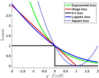
Graphical representation

We summarize the discussed losses in the Figure 1-1, where we renormalize some of them to pass through the point (1,0). The dashed line represents the regression formulation and solid ones are for classification problems.

-2 -1.5 -1 -0.5 0 0.5 1 1.5 2 0 0.5 1 1.5 2 2.5 3 Exponential loss Hinge loss 0-1 loss Logistic loss Square loss

Figure 1-1 – Graphical representation of classical loss functions. Contribution of this thesis

In Chapter 4 of this thesis we consider so-called Fenchel-Young losses for mul-ticlass linear classifiers, which extend convex surrogates to the mulmul-ticlass setting. This leads to saddle-point convex-concave problems with expensive matrix multipli-cations. Using stochastic optimization methods for non-Euclidean setup (using mirror descent) and specific variance reduction techniques we are able to reach sublinear (in the natural dimensionality of the problem) running time complexity per iteration.

(26)

1.2 Convex optimization

In this section we discuss the basics of convex optimization. Convexity is a pre-vailing setup for optimization problems, due to the theoretical guarantees for this class of functions. The classical convex minimization problem is the following:

min

𝑥∈𝒳 𝑓(𝑥),

where𝒳 ∈R𝑑is a convex set: for any two points𝑥, 𝑦 ∈ 𝒳 and for every𝛼∈[0,1]the

point 𝛼𝑥+ (1₋𝛼)𝑦 is also in _𝒳. This means, that for any two points inside the set,

the whole segment, connecting these points is also in the set. The function𝑓 is convex

as well: for any 𝑥, 𝑦 _{∈ 𝒳} and 𝛼_∈[0,1]: 𝑓(𝛼𝑥+ (1₋𝛼)𝑦)₆𝛼𝑓(𝑥) + (1₋𝛼)𝑓(𝑦) and this means, that the epigraph of function 𝑓 is a convex set: every chord lies above

the graph of a function. It is known for convex minimization problems, that: — If a local minimum exists, it is also a global minimum.

— The set of all global minima is convex (note, that global minimum is not necessarily unique).

Consider the unconstrained minimization problem, where𝒳 =_R𝑑_{. The first property}

provides us with the criterion of global minimum: if the function 𝑓 is differentiable,

then

∇𝑓(𝑥*) = 0 _⇔ 𝑥* is global minimum.

If the function𝑓 is not differentiable, we still can use the criterion, where the gradient

of the function is replaced by a sub-gradient: a generalization of gradient for convex function which defines the cone of directions in which the function increases [ Rock-afellar, 2015]:

𝜕𝑓(𝑥*)_∋0 _⇔ 𝑥* is global minimum.

However in practice, only for simple problems the solution can be found in closed form. For the majority of convex problems computational iterative methods are used, and the starting point for them are gradient descent or the steepest descent

𝑥𝑡+1 =𝑥𝑡₋𝛾𝑡∇𝑓(𝑥𝑡).

The idea is straightforward: we are looking for the direction in which the function increases and then descend in the opposite direction. Classical choices for stepsize are constant and decaying: 𝛾𝑡 =𝐶𝑡−𝛼, where 𝛼∈[0,1].

We also consider classical assumptions, such that bounded gradients, smoothness (which requires differentiability) and strong convexity (for more details see [Nesterov,

2013, Bubeck,2015]):

The first definition is the weakest one: bounded gradients, which does not require differentiability:

(27)

𝑥_{∈ 𝒳} and for any 𝑔(𝑥)_∈𝜕𝑓(𝑥):

‖𝑔(𝑥)_‖₆𝐵.

Definition 1.2. The function 𝑓 is called smooth with Lipschitz constant𝐿 if, for all 𝑥, 𝑦 _{∈ 𝒳}:

𝑓(𝑦)₆𝑓(𝑥) +_∇𝑓(𝑥)⊤(𝑦₋𝑥) + 𝐿

2‖𝑦−𝑥‖ 2

,

which is equivalent to, when 𝑓 is convex,

‖∇𝑓(𝑥)_{− ∇}𝑓(𝑦)_‖₆𝐿_‖𝑥₋𝑦_‖.

Definition 1.3. The function 𝑓 is called strongly convex with constant 𝜇 if, for all 𝑥, 𝑦 _{∈ 𝒳}:

𝑓(𝑦)_>𝑓(𝑥) +_∇𝑓(𝑥)⊤(𝑦₋𝑥) + 𝜇

2‖𝑦−𝑥‖ 2_.

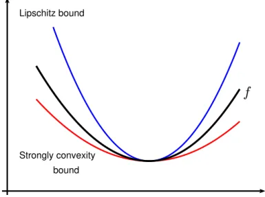
The intuitive definition of Lipschitz smoothness is that at every point, the function

𝑓 can be bounded above by quadratic function with coefficient 𝐿/2, strong convexity

means, that at every point the function 𝑓 is bounded below by quadratic function

with coefficient𝜇/2. A graphical representation of one dimensional case can be found in Figure 1-2.

Lipschitz bound

Strongly convexity bound

Figure 1-2 – Graphical representation of Lipschitz smoothness and strong convexity.

1.2.1 Euclidean geometry

Note, that we did not define norms for smoothness and strong convexity. If we define them as standard Euclidean norms, we reproduce the so-called Euclidean ge-ometry and constants𝐿and𝜇correspond to the biggest and the smallest eigenvalues

(28)

Projected gradient descent

The gradient descent method for constrained problem is called projected gradi-ent descgradi-ent (see [Bertsekas, 1999] and references therein) and one iteration is the following: 𝑥𝑡+1 = Π𝒳 (︀ 𝑥𝑡₋𝛾𝑡𝑔(𝑥𝑡) )︀ , with 𝑔(𝑥𝑡)_∈𝜕𝑓(𝑥𝑡) where Π𝒳(𝑥) = arg min

𝑦∈𝒳 ‖

𝑥₋𝑦_‖ is the Euclidean projection of the point𝑥 to the set

𝒳. We illustrate this approach in Figure 1-3. We can also to look at this equation

through the prism of proximal approaches [Moreau, 1965,Rockafellar,1976] as done for example in [Beck and Teboulle, 2003]:

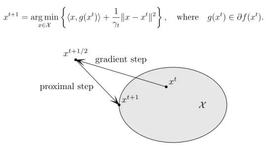
𝑥𝑡+1 = arg min 𝑥∈𝒳 {︂ ⟨𝑥, 𝑔(𝑥𝑡)_⟩+ 1 𝛾𝑡‖ 𝑥₋𝑥𝑡_‖2 }︂ , where 𝑔(𝑥𝑡)_∈𝜕𝑓(𝑥𝑡). xt xt+1/2 xt+1 X gradient step proximal step

Figure 1-3 – Graphical representation of projected gradient descent: firstly we do gradient step and then project onto 𝒳.

Note, that the proximal operator should be simple, i.e., the structure of the set 𝒳

be simple enough to compute it in either in closed form or with a number of iterations commensurate with the computation of the gradient.

Now we formulate main results for functions with different assumpions (short proofs can be found for example in [Bubeck, 2015]):

Theorem 1.1. Let 𝑓 be convex with bounded gradients with constant 𝐵; the radius

of set 𝒳 is 𝑅, i.e., sup

𝑥,𝑦∈𝒳‖

𝑥 ₋𝑦_‖ = 2𝑅. Then the projected gradient descent with

decaying stepsize 𝛾𝑡= _𝐵𝑅√_𝑡 satisfies:

𝑓(¯𝑥𝑡)₋𝑓(𝑥*)₆ 𝑅𝐵_√ 𝑡 , where 𝑥¯ 𝑡 = 1 𝑡 𝑡 ∑︁ 𝑖=1 𝑥𝑖.

(29)

Theorem 1.2. Let 𝑓 be convex and 𝐿-smooth on _𝒳. Then the projected gradient

descent with constant stepsize 𝛾𝑡= _𝐿1 satisfies:

𝑓(𝑥𝑡)₋𝑓(𝑥*)₆ 4𝐿‖𝑥 1₋_𝑥*

‖2

𝑡 .

Hence in case of 𝐿-smooth function we get an1/𝑡 convergence rate. If we add an

assumption about strong convexity of the function 𝑓, we recover exponential rate:

Theorem 1.3. Let 𝑓 be 𝜇 strongly convex and 𝐿-smooth on _𝒳. Then the projected

gradient descent with constant stepsize 𝛾𝑡= _𝐿1 satisfies: ‖𝑥𝑡+1₋𝑥*_‖2 ₆exp(︁₋𝑡_· 𝜇

𝐿 )︁

‖𝑥1₋𝑥*_‖2.

Note also that acceleration techniques, proposed by Nesterov can be used to in-crease the convergence rates. The first work in this direction [Nesterov, 1983] was proposed for smooth functions and unconstrained setup. It improved the rates from 1/𝑡 to1/𝑡2. The case of non-smooth function was considered in [Nesterov, 2005] and improved the rates from1/√𝑡 to1/𝑡, using a special smoothing technique, which can

be applied to functions with explicit max-structure. Constrained problems were con-sidered in [Nesterov,2007] and [Beck and Teboulle,2009] with the same convergence rates.

Note, that Theorems 1.1, 1.2 and 1.3 use Euclidean geometries: definitions of

smoothness and strongly convexity are given with respect with usual Euclidean ge-ometry. In the next section we extend these result for a more general setup.

1.2.2 Non-Euclidean geometry

The ideas of non-Euclidean approach are to exploit the geometry of the set 𝒳

and achieve the rates of projected gradient descent with constants adapting to the geometry of the set𝒳. Let us fix an arbitrary norm‖·‖X and a compact set𝒳 ∈R𝑑.

We introduce a definition of the dual norm:

Definition 1.4. The norm‖·‖X* is called the dual norm, if‖𝑔‖_X* = sup

𝑥∈_R𝑑_:_‖_𝑥_‖

X61

𝑔⊤𝑥.

Now we need to adapt definitions of bounded gradients, smoothness and strong convexity: (see for example [Bubeck,2015,Beck and Teboulle, 2003]) (i) we say, that function 𝑓(𝑥) has bounded gradients, if

‖𝑔_‖_X* 6𝐵 for any 𝑔(𝑥)∈𝜕𝑓(𝑥).

(ii) we say, that function 𝑓(𝑥) is𝐿-smooth with respect to norm _{‖ · ‖}_X if

(30)

where ‖ · ‖X* is dual norm, (iii) 𝜇-strongly convex if

𝑓(𝑦)_>𝑓(𝑥) +_∇𝑓(𝑥)⊤(𝑦₋𝑥) + 𝜇

2‖𝑦−𝑥‖ 2 X.

The idea of the mirror approach is to consider a so-called potential function Φ(𝑥) (which is also called DGF — distance generating function or mirror map), then switch to the mirror space (using gradient of potential), do the gradient step in this space, return back to the main space and project the point to the set𝒳.

Mirror descent

More formally, one step of Mirror descent [Nemirovsky and Yudin,1983] is

∇Φ(𝑥𝑡+1/2) =_∇Φ(𝑥𝑡)−𝛾𝑡∇𝑓(𝑥𝑡),

𝑥𝑡+1 _∈ΠΦ_𝒳(𝑥𝑡+1/2),

whereΠΦ

𝒳(𝑥, 𝑦) = arg min

𝑥∈𝒳

𝐵Φ(𝑥, 𝑦)is the projection in the Bregman divergence sense:

𝐵Φ(𝑥, 𝑦) = Φ(𝑥)−Φ(𝑦)− ∇Φ(𝑦)⊤(𝑥−𝑦). However, this notation could be difficult to embrace and [Beck and Teboulle, 2003] introduced the equivalent definition without switching to the mirror space, and one step of mirror descent can be written as:

𝑥𝑡+1 = arg min 𝑥∈𝒳 {︂ ⟨𝑥,_∇𝑓(𝑥𝑡)_⟩+ 1 𝛾𝑡 𝐵𝜑(𝑥, 𝑥𝑡) }︂ . (Mirror descent)

Note the similarity with projected gradient descent. In practice, the potentialΦ(𝑥) should be a strictly convex and differentiable function with the following properties:

— Φ(𝑥) is 1-strongly convex on _𝒳 with respect to _{‖ · ‖}_X.

— The effective square radius of set 𝒳, which is defined as Ω = sup

𝑥∈𝒳

Φ(𝑥) ₋ inf

𝑥∈𝒳Φ(𝑥)should be small.

— The proximal step above should be feasible.

Finally, we can formulate convergence rates for the Mirror descent algorithm for non-smooth case (a short proof can be found for example in [Bubeck,2015]):

Theorem 1.4. Let Φ be a 1-strongly convex with respect to _{‖ · ‖}_X and 𝑓 be convex

with 𝐵-bounded gradients with respect to _{‖ · ‖}_X. Then mirror descent with 𝛾𝑡= √ 2Ω 𝐵√𝑡 satisfies: 𝑓(¯𝑥𝑡)₋𝑓(𝑥*)₆𝐵 √︂ 2Ω 𝑡 , where 𝑥¯ 𝑡₌ 1 𝑡 𝑡 ∑︁ 𝑖=1 𝑥𝑖.

Note, that there are various extensions of mirror descent, such as mirror prox [ Ne-mirovski,2004], Dual Averaging [Nesterov, 2007] and extentions to saddle point min-imax problems [Juditsky and Nemirovski, 2011a,b, Nesterov and Nemirovski, 2013].

(31)

One more direction is NoLips approach, where the idea is to get rid of the Lipschitz-continuous gradient, using convexity condition which captures the geometry of the constraints [Bauschke et al.,2016].

Examples of geometries

ℓ2 geometry. This is the simplest geometry, which actually corresponds to the

Euclidean case. Indeed, in this case Φ(𝑥) = 1₂_‖𝑥_‖2

2 is 1-strongly convex with respect to the ℓ2 norm on the wholeR𝑑. The Bregman divergence, associated with this norm

is 𝐵𝜑(𝑥, 𝑦) = 1₂‖𝑥− 𝑦‖22 and one step of mirror descent is reduced to one step of projected gradient descent. Note, that Theorem1.4 is reduced to Theorem1.1in this case.

ℓ1 geometry. This is more interesting choice of geometry, which is also called sim-plex setup. If we define potential as negative entropy:

Φ(𝑥) =

𝑑

∑︁

𝑖=1

𝑥𝑖log𝑥𝑖,

then, using Pinsker’s inequality, we can show, that Φ is 1-strongly convex with re-spect to ℓ1 norm on the simplex ∆𝑑 = {𝑥 ∈ R𝑑+ :

𝑑

∑︀

𝑖=1

𝑥𝑖 = 1}. The Bregman

di-vergence associated with negative entropy is so-called he Kullback-Leibler didi-vergence:

𝐵𝜑(𝑥, 𝑦) = 𝐷KL(𝑥‖𝑦) = 𝑑

∑︀

𝑖=1

𝑥𝑖log 𝑥_𝑦𝑖

𝑖. The effective squared radius of ∆𝑑 is Ω = log𝑑

and moreover the solution for one step of MD can be found in closed form and lead to so-called multiplicative updates. This implies, that if we minimize function 𝑓 on the

simplex ∆𝑑, such that ‖∇𝑓‖∞ are bounded, the right choice of geometry give rates

as 𝑂(︀log𝑑 𝑡

)︀

, whereas the Euclidean geometry give rates only as 𝑂(︀_𝑑

𝑡

)︀ .

One more classical setup is often used: the ℓ1 ball can be obtained from the

simplex setup, by doubling the number of variables. Instead of 𝑑real values (positive

or negative), we consider 2𝑑 positive values and transform the 𝑑-dimensional ball to

the 2𝑑-dimensional simplex.

1.2.3 Stochastic setup

In this section we consider stochastic approaches going back to [Robbins and

Monro,1951], where we do not use the gradient∇𝑓(𝑥), but evaluate the noisy version of it: namely a stochastic oracle ̃︀𝑔(𝑥), such that E𝑔̃︀(𝑥) = ∇𝑓(𝑥). The classical setting in machine learning is when the objective function 𝑓 is the sampled mean of

observations 𝑓𝑖 (probably with some regularizer term):

𝑓(𝑥) = 1 𝑛 𝑛 ∑︁ 𝑖=1 𝑓𝑖(𝑥) +𝑅(𝑥),

(32)

and we can choose oracle as 𝑓𝑖(𝑥), where 𝑖 is chosen uniformly from 𝑛 points. In

fact, all negative log-likelihood minimization and loss minimization problems have this form. This also applies to the situation of single pass SGD where the bounds are then on the generalization error. To define the quality of an oracle ̃︀𝑔(𝑥), we assume the existence of the moment

𝐵2 = sup

𝑥∈𝒳E‖̃︀

𝑔(𝑥)_‖2_X*,

in the non-smooth case, and assume the existence of the variance in the smooth case:

𝜎2 = sup

𝑥∈𝒳E‖̃︀

𝑔(𝑥)_{− ∇}𝑓(𝑥)_‖2_X*,

where the norm depends on the geometry. Let us consider the general Stochastic Mirror Descent approach:

𝑥𝑡+1 = arg min 𝑥∈𝒳 {︂ ⟨𝑥,_̃︀𝑔(𝑥𝑡)_⟩+ 1 𝛾𝑡 𝐵𝜑(𝑥, 𝑥𝑡) }︂

. (Stochastic Mirror Descent)

Now we can formulate the theorem: [Juditsky et al., 2011,Lan, 2012,Xiao, 2010] Theorem 1.5. LetΦbe a 1-strongly convex with respect to _‖·‖𝒳 and𝐵2 be the second

moment of an oracle ̃︀𝑔(𝑥). Then Stochastic Mirror Descent with stepsize 𝛾𝑡 =

√ 2Ω 𝐵√𝑡 satisfies: E𝑓(¯𝑥𝑡)−𝑓(𝑥*)6𝐵 √︂ 2Ω 𝑡 , where 𝑥¯𝑡= 1 𝑡 𝑡 ∑︁ 𝑖=1 𝑥𝑖.

Note the similarity of this result with Theorem 1.4: the only difference is that bounded gradients are replaced with the bounded moment of the oracle.

1.3 Saddle point optimization

In this section we consider saddle point optimization. Consider two convex and compact sets 𝒳 ∈ R𝑑1 and 𝒴 ∈ R𝑑2. Let 𝜑(𝑥, 𝑦) : 𝒳 × 𝒴 → R be a function, such

that 𝜑(_·, 𝑦) is convex and 𝜑(𝑥,_·) is concave. The goal is to find min

𝑥∈𝒳max𝑦∈𝒴 𝜑(𝑥, 𝑦).

A classical example is obtained from Fenchel duality below. We present here results from [Juditsky and Nemirovski,2011a,b,Nesterov and Nemirovski,2013], concerning the mirror descent approach.

Introduce the (sub)gradient field: 𝐺(𝑥, 𝑦) = (︁𝜕𝑥𝜑(𝑥, 𝑦),−𝜕𝑦𝜑(𝑥, 𝑦)

)︁

— analogue of (sub)gradients for saddle point problems. Then subgradients are given by

(︁

(33)

The analogue of bounded gradients is written as:

Definition 1.5. Function 𝜑(𝑥, 𝑦) has bounded gradients, if _‖𝑔𝒳(𝑥, 𝑦)_‖𝒳* 6 ℒ_𝒳 and

‖𝑔𝒴(𝑥, 𝑦)_‖𝒴* 6ℒ_𝒴 for any (𝑥, 𝑦)∈(𝒳 × 𝒴).

To evaluate the quality of the point (_̃︀𝑥,𝑦_̃︀)_∈ (_{𝒳 × 𝒴}), we introduce the notion of the so-called duality gap:

Definition 1.6. The duality gap is ∆𝑑𝑢𝑎𝑙(̃︀𝑥,𝑦̃︀) = max

𝑦∈𝒴 𝜑(̃︀𝑥, 𝑦)−min𝑥∈𝒳 𝜑(𝑥,𝑦̃︀).

Observe, that the duality gap is the sum of the primal gapmax

𝑦∈𝒴 𝜑(𝑥, 𝑦̃︀ )−𝜑(𝑥 *_{, 𝑦}*₎

and the dual gap 𝜑(𝑥*, 𝑦*)₋min

𝑥∈𝒳 𝜑(𝑥,̃︀𝑦). Introduce the variable 𝑧 = (𝑥, 𝑦) and the set 𝒵 =_{𝒳 × 𝒴}. The main motivation of the duality gap is that it can be controlled in the following way, similar for the convex optimization:

∆𝑑𝑢𝑎𝑙(𝑧̃︀)6𝑔(̃︀𝑧) ⊤

(𝑧_̃︀₋𝑧),

where 𝑔(_̃︀𝑧)in the gradient field 𝐺(𝑧_̃︀), for more details see Bertsekas[1999].

Recall, that in order to apply mirror descent, we firstly need to construct potential and choose geometries. LetΦ𝒳(𝑥)be a potential, defined for variable the𝑥, such that

it is 1-strongly convex with respect to a norm ‖ · ‖X on 𝒳. Similarly, let Φ𝒴(𝑦) be

a potential, defined for the variable 𝑦, such that it is 1-strongly convex with respect

to a norm ‖ · ‖Y on𝒴. Let Ω𝒳 and Ω𝒴 be the effective square radii of sets𝒳 and 𝒴

with respect to the corresponding norms.

Let us construct the composite potential Φ𝒵(𝑧) = ℒ 𝒳 √ Ω𝒳 Φ𝒳(𝑥) + ℒ 𝒴 √ Ω𝒴 Φ𝒴(𝑦),then

one step of Saddle Point Mirror Descent (SP-MD) is the following:

𝑧𝑡+1 _∈arg min {︂ ⟨𝑔𝑡, 𝑧_⟩+ 1 𝛾𝑡 𝐵Φ𝒵(𝑧, 𝑧 𝑡₎ }︂ , 𝑔𝑡 _∈𝐺(𝑥𝑡, 𝑦𝑡) SP-MD Finally we can formulate the convergence rates:

Theorem 1.6. Let function 𝜑(𝑥, 𝑦) has a bounded gradients with constants _ℒ𝒳 and

ℒ𝒴. Then SP-MD with stepsize 𝛾𝑡 =

√︁ 2 𝑡 satisfies: max 𝑦∈𝒴 𝜑(¯𝑥 𝑡_{, 𝑦}₎ −min 𝑥∈𝒳 𝜑(𝑥,𝑦¯ 𝑡₎ 6(︁√︀Ω𝒳ℒ𝒳 + √︀ Ω𝒴ℒ𝒴 )︁√︂2 𝑡. Fenchel duality

We finish this introduction with the classical Fenchel duality result which provides us with the way to switch from convex problems to saddle-point problems. Let us firstly define the notion of the Fenchel conjugate of the convex function 𝑓:

(34)

Definition 1.7. The function 𝑓*(𝑦) given by 𝑓⋆₍_𝑦_{) := sup}_{⟨_{𝑦, 𝑥}_{⟩ −}_𝑓₍_𝑥₎_|_𝑥_∈

R𝑛}

is called the Fenchel conjugate of the function 𝑓.

Now we can formulate the theorem [see e.g. Borwein and Lewis, 2010]:

Theorem 1.7. (Fenchel’s duality theorem) Let 𝑓 : _{𝒳 →} _R and 𝑔 : _{𝒴 →} _R be

convex functions and 𝐴:_{𝒳 → 𝒴} be a linear map. Then

inf 𝑥∈𝒳 {︁ 𝑓(𝑥) +𝑔(𝐴𝑥) }︁ = sup 𝑦∈𝒴 {︁ −𝑓*(𝐴⊤𝑦)₋𝑔*(₋𝑦) }︁ .

Finally, we provide the way to switch between primal, dual and saddle point formulations of the convex problem:

Primal problem: inf

𝑥

{︁

𝑓(𝑥) +𝑔(𝐴𝑥) }︁

.

Dual problem: sup

𝑦

{︁

−𝑓*(𝐴⊤𝑦)₋𝑔*(₋𝑦)}︁.

Saddle problem: inf

𝑥 sup_𝑦

{︁

𝑓(𝑥)₋𝑔*(₋𝑦) +𝑦⊤𝐴𝑥}︁.

Machine learning motivation. These optimization problems are motivated by machine learning applications, where 𝑥 is the parameter to estimate, matrix 𝐴 the

data, 𝑔 the loss and 𝑓 the regularizer (note similarity with regularized empirical

risk minimization (1.1.1)). Dual or saddle problem formulations help to switch to an equivalent task, which in some sense has a simpler structure, like bilinear saddle-point problem with composite terms and moreover allows to control the duality gap.

(35)

(36)

Chapter 2

Sliced inverse regression with score

functions

Abstract

We consider non-linear regression problems where we assume that the response depends non-linearly on a linear projection of the covariates. We propose score func-tion extensions to sliced inverse regression problems, both for the first- order and second-order score functions. We show that they provably improve estimation in the population case over the non-sliced versions and we study finite sample estimators and their consistency given the exact score functions. We also propose to learn the score function as well, in two steps, i.e., first learning the score function and then learning the effective dimension reduction space, or directly, by solving a convex op-timization problem regularized by the nuclear norm. We illustrate our results on a series of experiments.

This chapter is based on the journal article: Slice inverse regression with score functions, D. Babichev, F. Bach, In Electronic Journal of Statistics [Babichev and Bach, 2018b].

2.1 Introduction

Non-linear regression and related problems such as non-linear classification are core important tasks in machine learning and statistics. In this chapter, we consider

a random vector 𝑥 _∈ _R𝑑, a random response _𝑦 _∈

R, and a regression model of the

form

𝑦=𝑓(𝑥) +𝜀, (2.1.1)

which we want to estimate from 𝑛 independent and identically distributed (i.i.d.)

observations (𝑥𝑖, 𝑦𝑖), 𝑖 = 1, . . . , 𝑛. Our goal is to estimate the function 𝑓 from these

data. A traditional key difficulty in this general regression problem is the lack of parametric assumptions regarding the functional form of 𝑓, leading to a problem of

(37)

a function𝑓 within an infinite-dimensional vector space.

While several techniques exist to estimate such a function, e.g., kernel methods, local-averaging, or neural networks [see, e.g., Györfi et al., 2002, Tsybakov, 2009], they also suffer from the curse of dimensionality, that is, the rate of convergence of the estimated function to the true function (with any relevant performance measure)

can only decrease as a small power of 𝑛, and this power cannot be larger than a

constant divided by 𝑑. In other words, the number 𝑛 of observations for any level of

precision is exponential in dimension.

A classical way of by-passing the curse of dimensionality is to make extra assump-tions regarding the function to estimate, such as the dependence on a lower unknown low-dimensional subspace, such as done by projection pursuit or neural networks. More precisely, throughout the chapter, we make the following assumption:

(A1) For all 𝑥 _∈_R𝑑, we have _𝑓₍_𝑥_{) =}_𝑔₍_𝑤⊤_𝑥₎_{for a certain matrix} _𝑤

∈ R𝑑×𝑘 and

a function 𝑔 :_R𝑘 _→ _R. Moreover, 𝑦 =𝑓(𝑥) +𝜀 with 𝜀 independent of 𝑥 with

zero mean and finite variance.

The subspace ofR𝑑spanned by the𝑘columns𝑤1, . . . , 𝑤𝑘∈R𝑑of𝑤has dimension

less than or equal to 𝑘, and is often called the effective dimension reduction (e.d.r.)

space. The model above is often referred to as a multiple-index model [Yuan, 2011]. We will always make the assumption that the e.d.r. space has exactly rank 𝑘, that is

the matrix 𝑤 has rank 𝑘 (which implies that𝑘 ₆𝑑).

Given𝑤, estimating𝑔may be done by any technique in non-parametric regression,

with a convergence rate which requires a number of observations𝑛 to be exponential

in 𝑘, with methods based on local averaging (e.g., Nadaraya-Watson estimators) or

on least-squares regression [see, e.g., Györfi et al., 2002, Tsybakov, 2009]. Given the non-linear function𝑔, estimating 𝑤is computationally difficult because the resulting

optimization problem may not be convex and thus leads to several local minima. The difficulty is often even stronger since one often wants to estimate both the function 𝑔

and the matrix𝑤.

Our main goal in this chapter is to estimate the matrix 𝑤, with the hope of

obtaining a convergence rate where the inverse power of 𝑛 will now be proportional

to 𝑘 and not 𝑑. Note that the matrix 𝑤 is only identifiable up to a (right) linear

transform, since only the subspace spanned by its column is characteristic.

Method of moments vs. optimization. This multiple-index problem and the goal of estimating 𝑤 only can be tackled from two points of views: (a) the method

of moments, where certain moments are built so that the effect of the unknown func-tion 𝑔 disappears [Brillinger,1982,Li and Duan,1989], a method that we follow here

and describe in more details below. These methods rely heavily on the model being correct, and in the instances that we consider here lead to provably polynomial-time algorithms (and most often linear in the number of observations since only moments are computed). In contrast, (b) optimization-based methods use implicitly or ex-plicitly non-parametric estimation, e.g., using local averaging methods to design an objective function that can be minimized to obtain an estimate of𝑤[Xia et al.,2002a,

(38)

descent techniques are used to obtain a local minimum. While these procedures offer no theoretical guarantees due to the potential unknown difficulty of the optimiza-tion problem, they often work well in practice, and we have observed this in our experiments.

In this chapter, we consider and improve a specific instantiation of the method of moments, which partially circumvents the difficulty of joint estimation by estimating

𝑤directly without the knowledge of𝑔. The starting point for this method is the work

by Brillinger [1982], which shows, as a simple consequence of Stein’s lemma [Stein,

1981], that if the distribution of 𝑥is Gaussian, (A1) is satisfied with 𝑘= 1 (e.d.r. of dimension one, e.g., a single-index model), and the input data have zero mean and identity covariance matrix, then the expectation E(𝑦𝑥) is proportional to 𝑤. Thus,

a certain expectation, which can be easily approximated given i.i.d. observations, simultaneously eliminates 𝑔 and reveals 𝑤.

While the result above provides a very simple algorithm to recover 𝑤, it has

several strong limitations: (a) it only applies to normally distributed data 𝑥, or more

generally to elliptically symmetric distributions [Cambanis et al., 1981], (b) it only applies to 𝑘 = 1, and (c) in many situations with symmetries, the proportionality constant is equal to zero and thus we cannot recover the vector 𝑤. This has led to

several extensions in the statistical literature which we now present.

Using score functions. The use of Stein’s lemma with a Gaussian random vari-able can be directly extended using the score function 𝒮1(𝑥) defined as the negative gradient of the log-density, that is, 𝒮1(𝑥) =−∇log𝑝(𝑥) = _𝑝−₍_𝑥1₎∇𝑝(𝑥), which leads to the following assumption:

(A2) The distribution of 𝑥 has a strictly positive density 𝑝(𝑥) which is differen-tiable with respect to the Lebesgue measure, and such that 𝑝(𝑥) _→ 0 when

‖𝑥_{‖ →}+_∞.

We will need the score to be sub-Gaussian to obtain consistency results. Given Assumption (A2), then Stoker[1986] showed, as a simple consequence of integration by parts, that, for 𝑘 = 1 and if Assumption (A1) is satisfied, then _E(𝑦_𝒮1(𝑥)) is proportional to 𝑤, for all differentiable functions 𝑔, with a proportionality constant

that depends on𝑤and_∇𝑔. This leads to the “average derivative method” (ADE) and

thus replaces the Gaussian assumption by the existence of a differentiable log-density,

which is much weaker. This however does not remove the restriction 𝑘 = 1, which

can be done in two ways which we now present.

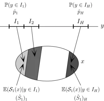
Sliced inverse regression. Given a normalized Gaussian distribution for 𝑥 (or

any elliptically symmetric distribution), then, if (A1) is satisfied, almost surely in 𝑦,

the conditional expectation E(𝑥|𝑦) happens to belong to the e.d.r. subspace. Given

several distinct values of𝑦, the vectors_E(𝑥_|𝑦) or any estimate thereof, will hopefully span the entire e.d.r. space and we can recover the entire matrix 𝑤, leading to “slice

inverse regression” (SIR), originally proposed by Li and Duan [1989], Duan and Li

[1991], Li[1991]. This allows the estimation with 𝑘 > 1, but this is still restricted to Gaussian data. In this chapter, we propose to extend SIR by the use of score functions

(39)

to go beyond elliptically symmetric distributions, and we show that the new method combining SIR and score functions is formally better than the plain ADE method. From first-order to second-order moments. Another line of extension of the simple method of Brillinger [1982] is to consider higher-order moments, namely the matrixE(𝑦𝑥𝑥⊤)∈R𝑑×𝑑, which, with normally distributed input data𝑥and, if (A1) is

satisfied, will be proportional (in a particular form to be described in Section2.2.2) to the Hessian of the function𝑔, leading to the method of “principal Hessian directions”

(PHD) from Li [1992]. Again, 𝑘 > 1 is allowed (more than a single projection), but thus is limited to elliptically symmetric data. HoweverJanzamin et al.[2014] proposed to used second-order score functions to go beyond this assumption. In order to define this new method, we consider the following assumption:

(A3) The distribution of 𝑥 has a strictly positive density 𝑝(𝑥) which is twice differentiable with respect to the Lebesgue measure, and such that 𝑝(𝑥) and

‖∇𝑝(𝑥)_{‖ →}0 when_‖𝑥_{‖ →}+_∞.

Given (A1) and (A3), then one can show [Janzamin et al., 2014] that E(𝑦𝒮2(𝑥)) will be proportional to the Hessian of the function 𝑔, where _𝒮2(𝑥) = ∇2log𝑝(𝑥) +

𝒮1(𝑥)𝒮1(𝑥)⊤ = _𝑝₍1_𝑥₎∇2𝑝(𝑥), thus extending the Gaussian situation above where 𝒮1 was a linear function and 𝒮2(𝑥), up to linear terms, proportional to𝑥𝑥⊤.

In this chapter, we propose to extend the method above to allow an SIR estimator for the second-order score functions, where we condition on 𝑦, and we show that the

new method is formally better than the plain method of Janzamin et al. [2014]. Learning score functions through score matching. Relying on score functions immediately raises the following question: is estimating the score function (when not available) really simpler than our original problem of non-parametric regression? Fortunately, a recent line of work [Hyvärinen,2005] has considered this exact problem, and formulated the task of density estimation directly on score functions, which is particularly useful in our context. We may then use the data, first to learn the score, and then to use the novel score-based moments to estimate 𝑤. We will also consider

a direct approach that jointly estimates the score function and the e.d.r. subspace, by regularizing by a sparsity-inducing norm.

Fighting the curse of dimensionality. Learning the score function is still a non-parametric problem, with the associated curse of dimensionality. If we first learn the score function (through score matching) and then learn the matrix 𝑤, we will not

escape that curse, while our direct approach is empirically more robust.

Note that Hristache, Juditsky and Spokoiny [Hristache et al., 2001] suggested iterative improvements of the ADE method, using elliptic windows which shrink in the directions of the columns of 𝑤, stretch in all others directions and tend to flat

layers orthogonal to 𝑤. Dalalyan, Juditsky and Spokoiny [Dalalyan et al., 2008]

generalize the algorithm to multi-index models and proved √𝑛-consistency of the

(40)

and weaker dependence for 𝑑 > 4. In particular, they provably avoid the curse of dimensionality. Such extensions are outside the scope of this chapter.

Contributions. In this chapter, we make the following contributions:

— We propose score function extensions to sliced inverse regression problems, both for the first-order and second-order score functions. We consider the infinite sample case in Section 2.2 and the finite sample case in Section 2.3. They provably improve estimation in the population case over the non-sliced versions, while we study in Section 2.3 finite sample estimators and their con-sistency given the exact score functions.

— We propose in Section 2.4 to learn the score function as well, in two steps, i.e., first learning the score function and then learning the e.d.r. space parameter-ized by 𝑤, or directly, by solving a convex optimization problem regularized

by the nuclear norm.

— We illustrate our results in 2.5 on a series of experiments.