Cable Parameters for Homogenous Cable-Beam Models
for Space Structures
Kaitlin Spak, Gregory Agnes, and Daniel Inman
Abstract In this paper, a method to determine the effective homogenous beam parameters for a stranded cable is presented.
There is not yet a predictive model for quantifying the structural impact of cable harnesses on space flight structures, and towards this goal, the authors aim to predict cable damping and resonance behavior. Cables can be modeled as shear beams, but the shear beam model assumes a homogenous, isotropic material, which a stranded cable is not. Thus, the cable-beam model requires calculation of effectively homogenous properties, including density, area, bending stiffness, and modulus of rigidity to predict the natural frequencies of the cable. Through a combination of measurement and correction factors, upper and lower bounds for effective cable properties are calculated and shown to be effective in a cable-beam model for natural frequency prediction.
Keywords Cable parameters • Cable modeling • Cable bending stiffness • Cable beam model • Cable vibration
Nomenclature
A Cross-sectional area c Viscous damping coefficient D Cable outer diameter d Individual wire diameter E Elastic modulus
EI Cable bending stiffness
Fs Transfer function matrix for use in distributed transfer function method
G Shear modulus
G(s) Hysteretic damping function I Moment area of inertia
k Spring stiffness, varies by cable size
L Beam length
M, N Left and right boundary condition matrices for distributed transfer function method r Layer diameter
Sysm System matrix
s Laplace transformed time coordinate T Axial tension in cable
Tm Transformation matrix t Time coordinate
K. Spak ()
Virginia Tech, Blacksburg, VA, USA e-mail:[email protected]
G. Agnes
Jet Propulsion Laboratory, California Institute of Technology, Pasadena, CA, USA D. Inman
Department of Aerospace Engineering, University of Michigan, Ann Arbor, MI, USA
F.N. Catbas (ed.), Dynamics of Civil Structures, Volume 4: Proceedings of the 32nd IMAC, A Conference and Exposition
on Structural Dynamics, 2014, Conference Proceedings of the Society for Experimental Mechanics Series,
DOI 10.1007/978-3-319-04546-7__2, © The Society for Experimental Mechanics, Inc. 2014
V Volume fraction
w Beam displacement as a function of time and distance
x Spatial coordinate; distance along the beam in the axial direction
ˇ Lay angle
State space vector of displacement solution and derivatives for distributed transfer function method Shear coefficient
Poisson’s ratio
Density
Angle between cable neutral axis and individual wire, as viewed from cable end Total beam rotation
2.1
Introduction
The control of space structures depends on accurate knowledge of their dynamic response to inputs. Thus, space structure models need to be high-fidelity and as realistic as possible to ensure accurate positioning. When lightweight structures are dressed with relatively heavy power and signal cables, the structures’ dynamic response changes [1,2]. In an effort to quantify and predict the dynamic response of cabled space structures, the study of cable dynamics is becoming increasingly important as requirements for dynamic mechanical stability of spacecraft become more stringent [3].
Cables used on spacecraft span a wide range of sizes, construction, and insulation. Currently, determination of cable parameters such as bending stiffness are performed experimentally through dynamic testing, and studies conducted to date used experimental data to back out the desired cable properties [4]. Ideally, cable parameters could be input into models based on basic measurements and properties of the cable rather than relying on experimental testing, which is more expensive and time consuming, and must be performed for each individual cable configuration. Therefore, this effort was conducted to determine how cable parameters could be simply calculated from wire measurements, material properties, and cable configuration.
In this paper, methods to determine cabled beam parameters a priori are presented. The cable parameters are used in a shear beam model to predict the natural frequencies of four types of cable. Comparison to experimental data to establish the validity of these methods concludes the paper.
2.2
Background
Cables can be modeled as shear beams [3]. Using a beam model is relatively straightforward and provides useful dynamic response data that can incorporate tension, internal damping and connection points. Beam models are not capable of determining internal friction forces directly, but instead rely on effective beam properties such as bending stiffness and damping to capture the frictional effects. Thus, determining these parameters to accurately portray the dynamic response is important.
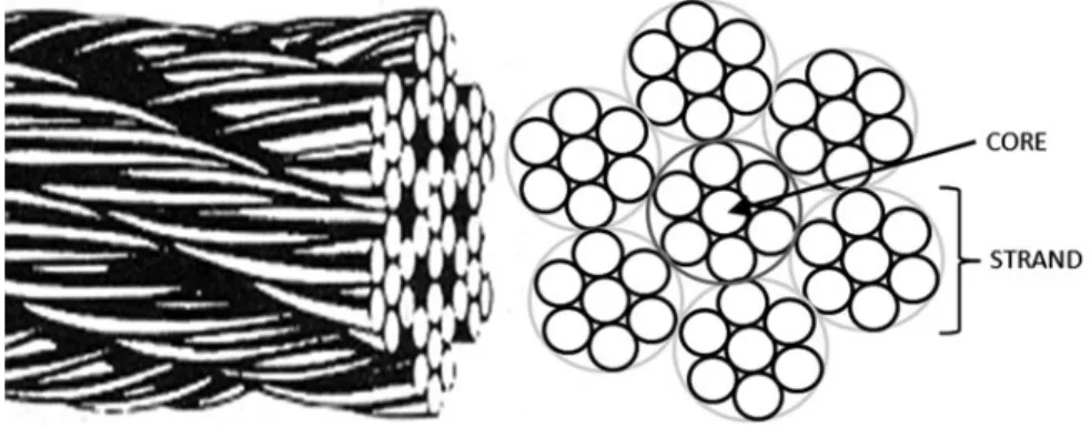
The cables used for space structures are generally made of an aluminum or copper core surrounded by EMI shielding and some type of electrical insulation. A core wire surrounded by layer wires is known as a strand. Cables have a core wire or strand surrounded by helically twisted wires or strands in successive layers. An “mn” designation is used to describe cable
Fig. 2.1 A 77 multi-strand cable consisting of a 17 core strand surrounded by a single layer of 17 strands
configuration, in which m is the number of strands and n is the number of wires in each strand. Figure2.1shows the layout of a 77 stranded cable comprising a 17 core and six 17 layer strands. Cables made up of wires in multiple small strands are more flexible than cables made up of a single strand with the same total number of wires. Cables may be helically twisted, in which each layer is wrapped in the same direction, or contra-helically twisted, in which the wrapping direction alternates with each successive layer. The lay angle is the angle that the layer wires makes with the core; cable lay angles generally range from 2.5ıto 35ı, with most mathematical analysis of cable behavior departing from reality beyond 20ı[5].
2.3
Cable Anatomy
The cable configurations investigated were 17, 119, 148, and 77, as shown in Fig.2.2. Five samples of each cable type were used, which were provided at cost by Southern California Braiding, Inc, a manufacturer of space-flight compatible cables. The cables were manufactured and wrapped on a planetary machine which ensured repeatability and uniformity between each sample. A contra-helical lay was used so that the cables would lay as straight as possible and natural curvature would not be a factor in the overall cable bending behavior. Cables were tied every 4–6 in. and wrapped with an outer layer of Kapton.
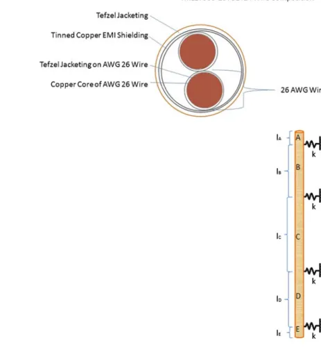
All of the cables used in this study were made with MIL27500-26TG2T14 wire. This wire, commonly used for space applications, consists of two 26AWG twisted wire pairs individually insulated, an EMI shield made of tinned copper, and outer Tefzel (ETFE) insulation layer. Figure2.3shows the components that make up the individual wire that is bundled together to make the cable. Figure2.4shows an idealized layout of the wire used for calculations. The wire has a left hand (s) lay and is shrink-wrapped with the Tefzel insulation, so there is an evident twist to the wire. The maximum and minimum wire diameters resulting from the twisting effect are averaged to give the effective wire diameter of 2.5 mm used throughout the study. Wire size measurements were taken from published values when possible [6] and verified with actual measurement. It is clear that the properties of the wire are different depending on whether the copper cores of the 26AWG wires are aligned with the horizontal (bending) axis or with the vertical axis.
Fig. 2.2 Cable configurations investigated for this study; from
left to right, 17, 119, 148, and 77
Fig. 2.3 Deconstructed cable wire, from top to bottom: Kapton wrapped cable, individual wire, and wire components: EMI shield, two 26AWG twisted wire pairs, and wire filler label
Fig. 2.4 Anatomy of MIL27500-26TG2T14 wire
Fig. 2.5 DTFM cable model configuration
2.4
Beam Model
Although there are many ways to model helical cables, for the purposes of determining dynamic response and interaction between cables and structures, a beam model has many advantages. Instead of modeling the forces in between the wires, which is difficult at best, the beam model assumes that the cable can be modeled as a homogenous cylindrical beam, with damping incorporated through damping terms of various forms and variable bending stiffness. The difficulty lies in determining the homogenous beam parameters to use, since a stranded cable is certainly neither isotropic nor homogenous. Past studies have “smeared” the cable properties across each layer to some success [7].
Since the ultimate goal of this work is to determine the effect of cable harnesses on the damping and dynamics of space structures, a model that can eventually incorporate the cable connection points is desirable. Thus, the distributed transfer function method (DTFM) was used to solve the beam model derived from the equation of motion. The distributed transfer function method provides exact solutions for the dynamic response of both branched and un-branched systems without requiring calculation of the system eigensolutions [8]. For the cables investigated here, an un-branched system was used with five segments and four mounting points, following the method of Yang [9]. Figure2.5shows the model configuration, designed to mimic the experimental test setup in terms of cable segments and boundary conditions.
The equation of motion is put into state space form and is combined with boundary condition matrices to form the characteristic equation. For an un-branched system such as a straight cable, the characteristic equation consists of the exponential of the state space matrix and transition matrices that relate the sections and include the spring connections to ground as shown in Fig.2.5.
To use the DTF method for a cable, the basic beam equation of motion is modified to include shear terms, a tension term, and damping terms (both viscous and hysteretic). The full equation of motion is:
A@ 2w @t2 EI G @4w @t2@x2 CEI @4w @x4 cEI AG @3w @t @x2 Z t 0 g .t /@ 4w @x4dtCc @w @t CT @2w @x2 D0
Here, wDw(x,t) is the transverse displacement of the cable and is a function of time, t, and distance, x. The coefficients , A, E, I,, and G are cable parameters discussed at length in the next section, while T is the cable tension and c is the viscous damping coefficient and g is a hysteretic damping form. Although damping is not yet considered in this investigation, the determination of damping parameters will be a future step, so they are included in the model.
The Laplace transform is taken of the equation of motion and the state space matrix is developed. Boundary condition matrices for the cable are modeled as free ends. Due to the inadequacies of a standard boundary condition model for representation of the interaction between the cable and a host structure [2], the free–free configuration was used with the connection points modeled as springs consisting of an aluminum tie down and cable tie component in series.
The state space matrix for the system is
Fs D 2 6 6 6 6 4 0 1 0 0 0 0 1 0 0 0 0 1 As2Ccs EIG.s/ s 0 EI s G CcEI sAGT EIG.s/ s 0 3 7 7 7 7 5
where G(s) is the hysteretic damping function, set to 0 for this study, as is the viscous damping constant c. Thus, the undamped state space matrix becomes
Fs D 2 6 6 4 0 1 0 0 0 0 1 0 0 0 0 1 A EIs 2 0 s G T EI 0 3 7 7 5
For the case of multiple system sections, the state space matrix is used for each section, along with a transformation matrix between sections. The transformation matrix is
TmD 2 6 6 4 1 0 0 0 0 1 0 0 0 kCcs EI 1 0 kcs EI 0 0 1 3 7 7 5
where the spring stiffness and damping terms represent the connection stiffness: k is the axial spring stiffness of the cable tie/TC 105 tab interface, k is the rotational spring stiffness, and the c terms are corresponding damping coefficients to be
determined with further experiments. The characteristic equation for the five-section cable model becomes det .MCN .Sysm//D0
which is solved numerically to yield natural frequencies for the system. M and N represent boundary conditions, in this case for a free–free configuration, and Sysmis the system matrix, consisting of a combination of the exponential of the Fsmatrix multiplied by each section length and transformation matrix as given by Sysm.
SysmDeFsl5TmeFsl4TmeFsl3TmeFsl2TmeFsl1
Displacements, mode shapes and frequency response functions can also be found through appropriate manipulation of the Sysmmatrix. The model was compared to published values for multi-span beams to ensure that it accurately captures the results due to the multiple pinned connections.
2.5
Cable Parameters
The cable parameters used in a shear beam model include bending stiffness (comprising both the modulus of elasticity and moment of inertia), density, area, modulus of rigidity, and shear coefficient. To predict the cable response, these values must be correlated to cable and wire properties such as modulus of elasticity and rigidity, cable geometry, and construction,
Table 2.1 Material properties
for cable components Property Copper Tefzel
Modulus of elasticity 110 GPa 1.2 GPa Modulus of rigidity 45 GPa 0.4 GPa Density 8,930 kg/m3 1,700 kg/m3
Poisson’s ratio 0.343 0.46
which forms the basis for our ongoing investigation. Bending stiffness is particularly important, since it can vary with cable curvature, tension, and wire slip. The wires are made up of essentially two components: copper, which makes up the conductor cores and EMI shielding, and Tefzel, the insulation for interior and exterior wires. The Kapton overwrap was assumed to add no additional stiffness other than keeping the cable wires in radial contact. Table2.1shows the material properties used for standard Tefzel-insulated copper cables.
Area is the most basic of the calculated parameters, but could still be calculated in myriad ways. For each beam property, values were calculated in several ways, ranging from calculations based on overall cable diameter (an over-estimation) to calculations based on individual wire components (an under-estimation). The middle value calculation, in which the overall wire diameter was used to find the area of a single wire and then multiplied by the number of wires in the cable, is commonly used for cross sectional area calculation.
Density was determined by weighing the cables and dividing by the volume, where the area was chosen to correspond to either the overall area, yielding a minimum density, the area calculated by summing the area of the wires, or the area calculated by summing the measured components comprising the wires. Thus, the minimumA value is given by using the maximum area to get a minimum density. Density values for the 119 cable were verified experimentally using Archimedes principle. It appears that the presence of air voids in the cable are taken into account more correctly when the overall volume of the cable is used for density calculations than when the wire component area is used.
The real contribution here comes from the calculation of the modulus values. Obviously, a stranded cable is quite different than a homogenous beam. The field of composite materials yielded useful approximations for wire properties; specifically, the individual wires that make up the cable could be modeled as a concentric cylinder composite, in which the copper conductor takes the role of the strengthening fiber and the Tefzel insulation takes the role of the matrix. Since the Tefzel insulation is tightly bonded to the conductor, the wire can reasonably be considered a composite material. Modulus value were based on a modified rule of mixtures for parallel fibers in a concentric matrix [10]. These expressions depend on the volume fraction of the copper in the wire, which was calculated by dividing the copper area (based on the area of the wire conductors and tinned copper shielding) by the area of the wire as a whole as determined by its outer diameter. For the wire used, vfD0.39528. The matrix fraction, calculated by area of Tefzel over total wire area was vmD0.432768, giving a void fraction of voD0.171952.
The shear modulus of a composite consisting of parallel fibers in a concentric matrix is given by GD 1Cvf Gf C 1vf Gm Gm Gf CGmvf Gf Gm
where vf is the volume fraction of the fiber and Gf and Gmare the shear moduli for fiber and matrix, respectively, where the copper acts as fiber and the Tefzel acts as matrix. This shear value is used for the cable as a whole. Further investigation may refine this value based on the interaction of individual wire shear profiles.
Bending stiffness of cables is considerably more complex; research shows that the bending stiffness of a beam is variable when the beam is a multi-stranded cable [11,12]. In this case, and in the case of space structure vibration, the amplitudes are small enough that there is virtually no slipping between the individual wires, so the bending stiffness approaches a maximum value which can be calculated as a function of the cable material and cable geometry. The bending stiffness for a stranded cable is given by Papailiou as the sum of the minimum bending stiffness plus additional stick or slip terms summed from each wire [11]. The minimum bending stiffness is
EImi nwi r eDEL
d4 64
where ELis the wire longitudinal modulus of elasticity (which itself must be determined by modeling the wire as a composite) and d is the diameter of the individual wire. The additional term to include the sticking between wires is
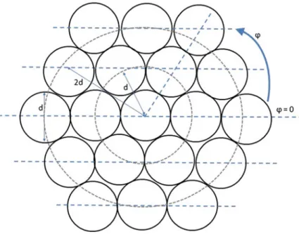
Fig. 2.6 119 cable end layout showing lines of inertia equivalence, layer diameters, and wire angles
where A is the wire area, r is the layer diameter,is the angle that the individual wire’s position makes with the horizontal (neutral) axis, andˇ is the lay angle. Figure 2.6shows the end layout of a 119 cable in which the layer diameters are noted in terms of the wire diameters, and the wire angle is shown starting at 0 radians at the horizontal axis and moving counterclockwise. The bending stiffness is calculated as the sum of the minimum stiffness, plus the stiffness of each additional layer. In the case of the 148 cable which does not have a complete layer, the average value between minimum stiffness (in which the additional layer wires are at the neutral axis) and maximum stiffness (in which additional layer wires are at the top and bottom of the cable) is used. The above bending stiffness equations are only applicable to single stranded concentric cables; for the multi-stranded 17 cable, the equations were modified to take into account the strand behavior of the outer layer. For the multi-stranded cable, the core EI is calculated as a single 17 strand and the outer strands are treated as large individual wires; in the EI wire stick formula, the base E value is used, the area is the area of the strand, r is the distance to the center wire in each strand,is the wire angle for the six outer strand center wires andˇis the lay angle for the strands, not the individual wires. This approach, though novel, worked well; smearing the outer strands as large wires resulted in a lower overall bending stiffness for the multi-stranded cable than the similarly sized single stranded cable, which agreed with experimental data and theory.
To determine the wire modulus of elasticity, the concentric composite model was used [9]. For a beam in bending, the longitudinal modulus of elasticity is used, given by
ELDvfEf CvmEmC 2vf vm 2 EmEfvf 1vf Em.1vm/ 1vf 2v2f C1vm2v2m vmC.1Cvm/ Ef
The modulus for copper and Tefzel are used for the fiber and matrix, and the base longitudinal modulus for a single wire is calculated. However, this expression applies for straight parallel fibers; in the case of a twisted conductor pair, the modulus of elasticity is reduced by as much as 10 %. Thus, a 0.9 factor is included in the wire elastic modulus to take into account this fiber curvature effect.
Another aspect to the model was the calculation of the tie down stiffness. Although past studies determined tie down stiffness through experimental comparison of a known system, the extremely stiff value calculated for finite element analysis in [3] did not represent the experimental connection points well. In addition, experiments performed by the author and colleagues resulted in a wide variety of stiffness values and poor repeatability, so it is clear that further study is required to characterize the connection stiffness. Tie down stiffnesses were also calculated theoretically. The stiffness of the aluminum TC 105 tab was combined in series with the stiffness of the nylon cable tie for each cable size, assuming good contact all the way around the cable. Since this connection stiffness affects the natural frequencies directly, the results presented here are likely to change with increased confidence in the tie down stiffness values. A rotational degree of freedom and both axial and rotational spring damping were added to the model so that the connection can be more correctly represented with more study. Since the cable is modeled as a free–free beam, when the stiffness is very low (essentially zero), there is a rigid body mode;
Table 2.2 Effect of spring
stiffness on frequency Frequency (rad)
k (N/m) 1 2 3 11a 28 232 639 3,245a 389 472 545 7,638b 574 697 783 93,400c 1,118 1,489 >2,000 525,000d 1,147 >2,000 >2,000 aValues calculated experimentally bTheoretical value
cAuthor experimental value dAFRL experimental value [3]
Fig. 2.7 Cable test set up; two end pieces, two buffer zones and a center test section make up the five model cable segments
as the stiffness increases, the rigid body mode moves away from zero. As the stiffness further increases, the initial frequency increases and then splits into multiple frequencies, which matched with the larger cables’ responses well. Table2.2shows the effect of increasing spring stiffness on the first three modes in which it is clear that the spring stiffness affects frequency greatly. For the results presented, stiffness values were chosen based on the experimental results of the author.
2.6
Experimental Comparison
Of course calculating the theoretical cable parameters is only the first step; we must know that these theoretical values are capable of modeling the cable and producing frequency values that are similar to those experimentally found. Each cable was mounted in a test fixture using the same tie-down tabs that the cables would see in space structure assemblies. The cable was “pinned” in four places to make three sections, a center test section and two buffer sections to mitigate end effects. A tensioned wire was used to excite the cable, and a load cell measured the input force while a laser vibrometer measured the output velocity. From these values, a transfer function was obtained for each trial. Five samples of each type of cable were tested between 12 and 14 times, for a total of 60–70 trials per cable type. Figure2.7shows the cable test set up with test and buffer zones identified. Further details on the development of this test are available in [13]. Frequency response functions for the cables always showed a clear first mode that represented bending of the test section, variable frequency and mode number interaction modes in which the bending frequencies of the buffer sections came into play, and a clear higher frequency mode in which the test section showed pure second frequency beam bending.
2.7
Results
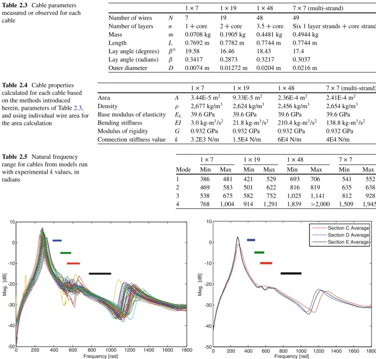
The variety of cable parameters were calculated for each of the four cable types based on the cable measurements. Table2.3
gives the measured values; note that these are all simple measurements that can be taken with a ruler and a scale. Table2.4
gives the middle values calculated for each cable, and Table2.5gives the maximum and minimum values for the first four frequencies for the specific k value for each cable given in Table2.4. Figures2.8,2.9,2.10, and2.11show the experimental results with the first four frequency ranges overlaid with range bars; the larger cables showed multiple peaks near the first beam mode, and seem to be modeled more appropriately with the stiff connection values that cause additional frequencies at the first mode. It is noted that results are best for larger, more beam like cables; this agrees with previously published work that found that the calculation of bending stiffness became more accurate as the number of wires in a given layer increases [14].
Table 2.3 Cable parameters measured or observed for each cable
17 119 148 77 (multi-strand) Number of wires N 7 19 48 49
Number of layers n 1Ccore 2Ccore 3.5Ccore Six 1 layer strandsCcore strand Mass m 0.0708 kg 0.1905 kg 0.4481 kg 0.4944 kg
Length L 0.7692 m 0.7782 m 0.7744 m 0.7744 m Lay angle (degrees) ˇı 19.58 16.46 18.43 17.4 Lay angle (radians) ˇ 0.3417 0.2873 0.3217 0.3037 Outer diameter D 0.0074 m 0.01272 m 0.0204 m 0.0216 m
Table 2.4 Cable properties calculated for each cable based on the methods introduced herein, parameters of Table2.3, and using individual wire area for the area calculation
17 119 148 77 (multi-strand) Area A 3.44E-5 m2 9.33E-5 m2 2.36E-4 m2 2.41E-4 m2
Density 2,677 kg/m3 2,624 kg/m3 2,456 kg/m3 2,654 kg/m3
Base modulus of elasticity EL 39.6 GPa 39.6 GPa 39.6 GPa 39.6 GPa
Bending stiffness EI 3.0 kg-m3/s2 21.8 kg-m3/s2 210.4 kg-m3/s2 138.8 kg-m3/s2
Modulus of rigidity G 0.932 GPa 0.932 GPa 0.932 GPa 0.932 GPa Connection stiffness value k 3.2E3 N/m 1.5E4 N/m 6E4 N/m 4E4 N/m
Table 2.5 Natural frequency range for cables from models run with experimental k values, in radians
17 119 148 77
Mode Min Max Min Max Min Max Min Max 1 386 481 421 529 693 706 541 552 2 469 583 501 622 816 819 635 638 3 538 675 582 752 1,025 1,141 812 928 4 768 1,004 914 1,291 1,839 >2,000 1,509 1,945 0 200 400 600 800 1000 1200 1400 1600 1800 -50 -40 -30 -20 -10 0 10 Frequency [rad] Mag. [dB] 0 200 400 600 800 1000 1200 1400 1600 1800 -50 -40 -30 -20 -10 0 10 Frequency [rad] Mag. [dB] Section C Average Section D Average Section E Average
Fig. 2.8 17 experimental data frequency response functions with frequency range bars for the first four frequencies shown over individual trial runs (left) and averaged runs for each section (right) (color figures online)
200 400 600 800 1000 1200 1400 1600 1800 2000 -50 -45 -40 -35 -30 -25 -20 -15 -10 -5 0 Frequency [rad] Mag. [dB] 200 400 600 800 1000 1200 1400 1600 1800 2000 -50 -45 -40 -35 -30 -25 -20 -15 -10 -5 0 Frequency [rad] Mag. [dB] Section A Average Section B Average Section C Average
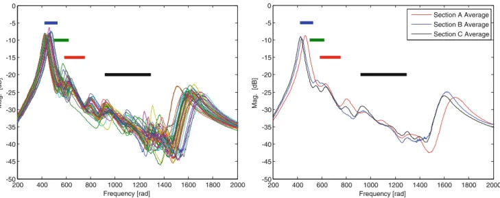
Fig. 2.9 119 experimental data frequency response functions with frequency range bars for the first four frequencies shown over individual trial runs (left) and averaged runs for each section (right)
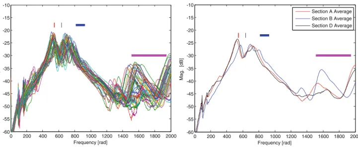
200 400 600 800 1000 1200 1400 1600 1800 2000 -60 -55 -50 -45 -40 -35 -30 -25 -20 -15 -10 Frequency [rad] Mag. [dB] 200 400 600 800 1000 1200 1400 1600 1800 2000 -50 -45 -40 -35 -30 -25 -20 -15 -10 Frequency [rad] Mag. [dB] Section B Average Section D Average Section E Average
Fig. 2.10 148 experimental data frequency response functions with frequency range bars for the first four frequencies shown over individual trial runs (left) and averaged runs for each section (right)
Some difficulty arises in comparison of the model results to the experimental data because of the inherent variation in cable behavior. Although all of the cables show clear large frequency response function peaks at the first bending mode of the center section, the interaction modes between the first and second center section beam modes are erratic; for instance, one section of cable might show two interaction modes between the first and second center section beam modes, while another section of the same type of cable shows three. Even within the results from the same cable section the number of interaction modes varies. In Figs.2.8,2.9,2.10, and2.11, the left hand side shows all of the individual trial runs to demonstrate the variability from trial to trial, while the right side of the figures show the averages for each section of each type of cable. It is clear that a statistical analysis could be beneficial to determine whether the model is capturing the interaction modes correctly. For now, comparison was largely based on whether the model result values were in the neighborhood of the first frequency of the experimental data, which was the case for the medium and large cables. The 17 cables’ frequency values had a greater spread in experimental trials than predicted by the model.
For the 17 cable, the first model frequency (represented by top blue bar in Fig.2.8) was predicted too high; inclusion of damping, which would affect the first mode the most, may adjust this prediction accordingly. The second and third frequencies (next highest green and red bars, respectively) correspond to the interaction modes between 400 and 700 radians, and the fourth frequency, shown as the bottom black bar, is too low to accurately predict the corresponding cable frequency. Thus, the 17 cable model as it is may be useful for determining the interaction modes but provides a poor prediction for
0 200 400 600 800 1000 1200 1400 1600 1800 2000 -60 -55 -50 -45 -40 -35 -30 -25 -20 -15 -10 Frequency [rad] Mag. [dB] 0 200 400 600 800 1000 1200 1400 1600 1800 2000 -60 -55 -50 -45 -40 -35 -30 -25 -20 -15 -10 Frequency [rad] Mag. [dB] Section A Average Section B Average Section D Average
Fig. 2.11 77 experimental data frequency response functions with frequency range bars for the first four frequencies shown over individual trial runs (left) and averaged runs for each section (right)
the major cable bending modes. However, it is possible that the fourth model frequency may still be an interaction mode, and that further values should be compared to predict the pure test second bending mode.
The 119 cable results in Fig.2.9showed good agreement for the first mode, and interaction modes were captured adequately. In this case, the fourth frequency is likely to correspond to interaction modes rather than the second pure bending mode of the test section. The broad range of the fourth model frequency may incorporate multiple interaction modes.
The larger 148 and 77 cables showed a marked decrease in range for the first two modeled frequencies, which corresponded well to the multiple two or three large peaks of the cables’ frequency response functions. The 77 model showed the best agreement, giving credibility to the novel strand bending stiffness calculation method presented earlier. However, it is clear with the larger cables that the variability from section to section and even trial to trial is quite large, with varying numbers of modes at certain frequencies. Even with the narrower range, the modeled frequencies are approximations at best and may not capture all of the small interaction frequencies that are evident.
2.8
Conclusion and Future Work
Effective beam parameters were determined to model non-homogenous cables as homogenous beams. Cable area was calculated through one of three approaches, which were carried through calculations for the volume fraction of materials, cable density, bending stiffness, and shear modulus. An upper and lower bound was determined for the first four frequencies of four types of cables for certain connection stiffness values, but further investigation into the connection stiffness is required for accurate comparison of the model to the experimental data. In addition, the high variability between cable sections and trials indicate that a statistical approach may be necessary to interpret any model with confidence, as the number of modes is variable from trial to trial. In addition to creating a statistical analysis to analyze the experimental cable behavior, the next step involves adding damping to the model; by determining the viscous and hysteretic damping parameters, a more accurate model can be developed, and the additional dissipation facilitated by the cable attachments can be quantified.
Acknowledgements This work was supported by a NASA Office of the Chief Technologist’s Space Technology Research Fellowship. Cables for experimental validation were provided at cost by Southern California Braiding Co. The third author gratefully acknowledges the support of AFOSR Grant number FA9550-10-1-0427 monitored by Dr. David Stargel. Part of this research was carried out at the Jet Propulsion Laboratory, California Institute of Technology, under a contract with the National Aeronautics and Space Administration.
References
1. Goodding J, Babuska V, Griffith DT, Ingram BR, Robertson LM (2008) Studies of free–free beam structural dynamics perturbations due to mounted cable harnesses. In: 48th AIAA/ASME/ASCE/AHS structures, structural dynamics and materials conference, AIAA-2008–1852, April 2008
2. Coombs DM, Goodding JC, Babuska V, Ardelean EV, Robertson LM, Lane SA (2011) Dynamic modeling and experimental validation of a cable-loaded panel. J Spacecr Rockets 48(6):958–972
3. Babuska V, Coombs DM, Goodding JC, Ardelean EV, Robertson LM, Lane SA (2010) Modeling and experimental validation of space structures with wiring harnesses. J Spacecr Rockets 47(6):1038–1052
4. Goodding JC, Ardelean EV, Babuska V, Robertson LM, Lane SA (2011) Experimental techniques and structural parameter estimation studies of spacecraft cables. J Spacecr Rockets 48(6):942–957
5. Ghoreishi SR, Messager T, Cartraud P, Davies P (2007) Validity and limitations of linear analytical models for steel wire strands under axial loading, using a 3D FE model. Int J Mech Sci 49:1251–1261
6. Military specification MIL-C-27500G: cable, power, electrical and cable special purpose electrical shielded and unshielded. General Specification for, May 1988http://www.everyspec.com/MIL-SPECS/MIL-SPECS-MIL-C/MIL-C-27500G_47023/
7. Jolicoeur C, Cardou A (1996) Semicontinuous mathematical model for bending of multilayered wire strands. J Eng Mech 122(7):643–650 8. Yang B, Tang CA (1992) Transfer functions of one-dimensional distributed parameter systems. J Appl Mech 59:1009–1014
9. Yang B (2010) Exact transient vibration of stepped bars, shafts, and strings carrying lumped masses. J Sound Vib 329:1191–1207
10. Sendeckyj GP (1974) Elastic behavior of composites, vol 2, Mechanics of composite materials. Academic, New York, pp 45–83 (Chapter 3) 11. Papailiou KO (1997) On the bending stiffness of transmission line conductors. IEEE Trans Power Deliv 12(4):1576–1588
12. Knapp RH, Liu X (2005) Cable vibration considering interlayer coulomb friction. Int J Offshore Polar Eng 15(3):229–234
13. Spak KS, Agnes GS, Inman DJ (2013) Toward modeling of cable harnessed structures: cable damping experiments. In: 54th AIAA/ASME/ASCE/AHS/ASC structures, structural dynamics, and materials conference, Boston, AIAA-2013–1889, April 2013