Stochastic Optimization for Big Data Analytics: Algorithms and Libraries

Stochastic Optimization for Big Data Analytics:

Algorithms and Libraries

Tianbao Yang‡

SDM 2014, Philadelphia, Pennsylvania

collaborators:

Rong Jin†, Shenghuo Zhu‡ ‡_{NEC Laboratories America,}†_{Michigan State University}

http://www.cse.msu.edu/~yangtia1/sdm14-tutorial.pdf

Outline

1 STochastic OPtimization (STOP) and Machine Learning

2 STOP Algorithms for Big Data Classification and Regression

3 General Strategies for Stochastic Optimization

Introduction

Machine Learning problems and Stochastic Optimization Coverage:

Classification and Regression in different forms

Motivation to employSTochasticOPtimization (STOP) Basic Convex Optimization Knowledge

Learning as Optimization

Least Square Regression Problem:

min w∈Rd 1 n n X i=1 (yi−w>xi)2+ λ 2kwk 2 2

xi ∈Rd: d-dimensional feature vector

yi ∈R: response variable

w∈_Rd_{: unknown parameters}

Learning as Optimization

Least Square Regression Problem:

min w∈Rd 1 n n X i=1 (yi−w>xi)2 | {z } Empirical Loss +λ 2kwk 2 2

xi ∈Rd: d-dimensional feature vector

yi ∈R: response variable

w∈_Rd_{: unknown parameters}

Learning as Optimization

Least Square Regression Problem:

min w∈_Rd 1 n n X i=1 (yi−w>xi)2+ λ 2kwk 2 2 | {z } Regularization

xi ∈Rd: d-dimensional feature vector

yi ∈R: response variable

w∈_Rd_{: unknown parameters}

Learning as Optimization

1. SVMs: hinge loss`(z) = max(0,1−z)p<sub>, wherep= 1,2</sub> 2. Logistic Regression: `(z) = log(1 + exp(−z))

Learning as Optimization

Learning as Optimization

Feature Selection usingElastic Net:

min w∈_Rd 1 n n X i=1 `(yiw>xi)+λ kwk1+γkwk22

Big Data Challenge

Huge amount of data generated on the

internet every day

Facebook users upload3 million photos

Goolge receives3000 million queries

GE100 MillionHours of operational data on the World’s Largest Gas Turbine Fleet

The global internet population is2.1

billionpeople

http://www.visualnews.com/2012/06/19/ how-much-data-created-every-minute/

Why Learning from Big Data is Hard?

empirical loss + regularizer

Too many data points

Issue: can’t afford go through data set many times

Why Learning from Big Data is Hard?

empirical loss + regularizer

High Dimensional Data

Issue: can’t afford second order optimization (e.g. Newton’s method)

Why Learning from Big Data is Hard?

empirical loss + regularizer

Data are distributed over many machines

Issue: expensive (if not impossible) to move data

Warm-up: Vector, Norm, Inner product, Dual Norm

bold letters x∈_Rd_,w∈

Rd : d-dimensional vectors

normkxk: Rd→R+. e.g. `2 normkxk2=

q Pd i=1xi2,`1 norm kxk<sub>1</sub>=Pd i=1|xi|,`∞ normkxk∞= maxi|xi| inner product <x,y>=x>y=Pd i=1xiyi

Warm-up: Convex Optimization

Warm-up: Convergence Measure

Most optimization algorithms are iterative

wt+1 =wt+ ∆wt

Iteration Complexity: the number of iterationsT() needed to have

f(xT)−min

x∈Xf(x)≤ (1)

Convergence rate: afterT iterations, how good is the solution

f(xT)−min x∈Xf(x)≤(T) 0 20 40 60 80 100 0 0.2 0.4 0.6 0.8 1 objective ε(T) Optimal Value

More on Convergence Measure

Convergence Rate Iteration Complexity

linear µT _{(µ <1) O log(}1 ) sub-linear _T1α α >0 O 1 1/α

More on Convergence Measure

Convergence Rate Iteration Complexity

linear µT _{(µ <1) O log(}1 ) sub-linear _T1α α >0 O 1 1/α

More on Convergence Measure

Convergence Rate Iteration Complexity

linear µT (µ <1) O log(1) sub-linear _T1α α >0 O 1 1/α 20 40 60 80 100 0 0.05 0.1 0.15 0.2 0.25 0.3 iterations

distance to optimal objective

More on Convergence Measure

Convergence Rate Iteration Complexity

linear µT (µ <1) O log(1) sub-linear _T1α α >0 O 1 1/α 20 40 60 80 100 0 0.05 0.1 0.15 0.2 0.25 0.3 iterations

distance to optimal objective

0.5T

More on Convergence Measure

Convergence Rate Iteration Complexity

linear µT (µ <1) O log(1) sub-linear _T1α α >0 O 1 1/α 20 40 60 80 100 0 0.05 0.1 0.15 0.2 0.25 0.3 iterations

distance to optimal objective

0.5T

1/T2

More on Convergence Measure

Convergence Rate Iteration Complexity

linear µT (µ <1) O log(1) sub-linear _T1α α >0 O 1 1/α 20 40 60 80 100 0 0.05 0.1 0.15 0.2 0.25 0.3 iterations

distance to optimal objective

0.5T

1/T2

1/T

More on Convergence Measure

Convergence Rate Iteration Complexity

linear µT (µ <1) O log(1) sub-linear _T1α α >0 O 1 1/α 20 40 60 80 100 0 0.05 0.1 0.15 0.2 0.25 0.3 iterations

distance to optimal objective

0.5T 1/T2 1/T 1/T0.5 µT < 1 T2 < 1 T < 1 √ T log 1 < √1 < 1 < 1 2

Factors that affect Iteration Complexity

Domain X: size and geometry

Size of problem: dimension and number of data points

Warm-up: Non-smooth function

Lipschitz continuous: e.g. absolute loss f(z) =|z|

|f(x)−f(y)| ≤Lkx−yk f(x)≥f(y) +∂f(y)>(x−y) −1 −0.5 0 0.5 1 −0.2 0 0.2 0.4 0.6 0.8 |x| non−smooth sub−gradient Iteration complexityO 1 2 or convergence rateO 1 √ T

Warm-up: Smooth Convex function

smooth: e.g. logistic lossf(z) = log(1 + exp(−z))

k∇f(x)− ∇f(y)k∗ ≤βkx−yk

whereβ >0

Second Order Derivative is upper

bounded −0.2−1 −0.5 0 0.5 1 0 0.2 0.4 0.6 0.8 x2 gradient smooth

Full gradient descentO

1 √ orO 1 T2

Stochastic gradient descent O

1 2 or O 1 √ T

Warm-up: Strongly Convex function

strongly convex: e.g. `2₂ normf(x) = 1₂kxk2 2

k∇f(x)− ∇f(y)k∗≥λkx−yk, λ >0 Second Order Derivative is lower bounded

Warm-up: Smooth and Strongly Convex function

smooth and strongly convex:

λkx−yk ≤ k∇f(x)− ∇f(y)k∗ ≤βkx−yk, β ≥λ >0

e.g. square loss: f(z) = 1₂(1−z)2

Iteration complexityO log 1 or convergence rateO(µT)

Warm-up: Stochastic Gradient

Loss:

whereit ∈ {1, . . . ,n} randomly sampled key equation: Eit[∇`(w>xit,yit)] =∇L(w)

Warm-up: Dual

Dual Objective (classification):

min w 1 n n X i=1 `(yiw>xi | {z } z ) +λ 2kwk 2 2 = min w 1 n n X i=1 max αi∈Ω αi(yiw>xi)−`∗(αi) +λ 2kwk 2 2 = max α∈Ω 1 n n X i=1 −`∗(αi)− λ 2 1 λn X i=1 αiyixi 2 2

Outline

1 STochastic OPtimization (STOP) and Machine Learning

2 STOP Algorithms for Big Data Classification and Regression

3 General Strategies for Stochastic Optimization

STOP Algorithms for Big Data Classification and

Regression

In this section, we present several well-known STOP algorithms for solving classification and regression problems

Coverage:

Stochastic Gradient Descent (Pegasos) forL1-SVM(primal) Stochastic Dual Coordinate Ascent (SDCA) forL2-SVM(dual) Stochastic Average Gradient (SAG) forLogistic Regression/Regression

STOP Algorithms for Big Data Classification

Support Vector Machines:

min w∈_Rdf(w) = 1 n n X i=1 `(w>xi,yi) | {z } loss +λ 2kwk 2 2 −1 −0.5 0 0.5 1 1.5 2 0 0.5 1 1.5 2 2.5 3 3.5 4 ywTx loss L1−SVM L2−SVM non−smooth function smooth function L1 SVM:`(w>x,y) = max(0,1−yiw>xi) L2 SVM:`(w>x,y) = max(0,1−yiw>xi)2 Equivalent to C-SVM formulationsC =nλ

STOP Algorithms for Big Data Classification

Support Vector Machines:

min w∈_Rdf(w) = 1 n n X i=1 `(w>xi,yi) | {z } loss +λ 2kwk 2 2 −1 −0.5 0 0.5 1 1.5 2 0 0.5 1 1.5 2 2.5 3 3.5 4 ywTx loss L1−SVM L2−SVM non−smooth function smooth function L1 SVM:`(w>x,y) = max(0,1−yiw>xi) L2 SVM:`(w>x,y) = max(0,1−yiw>xi)2 Equivalent to C-SVM formulationsC =nλ

STOP Algorithms for Big Data Classification

Support Vector Machines:

min w∈_Rdf(w) = 1 n n X i=1 `(w>xi,yi) | {z } loss +λ 2kwk 2 2 −1 −0.5 0 0.5 1 1.5 2 0 0.5 1 1.5 2 2.5 3 3.5 4 ywTx loss L1−SVM L2−SVM non−smooth function smooth function L1 SVM:`(w>x,y) = max(0,1−yiw>xi) L2 SVM:`(w>x,y) = max(0,1−yiw>xi)2 Equivalent to C-SVM formulationsC =nλ

Pegasos (

, primal): STOP for L

SVM

Pegasos (SGD for strongly convex) :

stochastic gradient: ∂`(w>xi,yi) =    −yixi, 1−yiw>xi <0 0, otherwise ∂f(wt;it) =∂`(wt>xit,yit) +λwt

Stochastic Gradient Descent Updates

wt+1=wt−

1

SDCA (

, dual): STOP for

L

SVM

convex conjugate: max(0,1−yw>x)2 = max

α≥0 α−1 4α 2 −αyw>x Dual SVM: max α≥0 D(α) = 1 n n X i=1 αi− α2_i 4 | {z } φ∗_(α i) −λ 2 1 λn n X i=1 αiyixi 2 2 primal solution: wt= 1 λn n X i=1 αt_iyixi SDCA: stochastic dual coordinate ascent

Dual Coordinate Updates

∆αi = max αt i+∆αi≥0 φ∗(αt_i + ∆αi)− λ 2 wt+ 1 λn∆αiyixi 2 2

SAG (

, primal): Stopt for Logit Reg./ Reg.

smooth and strongly convex objective min w∈Rd f(w) = 1 n n X i=1 `(w>xi,yi) + λ 2kwk 2 2 | {z }

smooth and strongly convex

e.g. logistic regression, least square regression

SAG (stochastic average gradient):

wt+1 = (1−ηλ)wt− η n n X i=1 g_it , where g_it =    ∂`(w>_t xi,yi), if i is selected g_it−1, otherwise

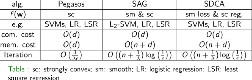
OK, tell me which one is the best?

Let us compare Theoreticallyfirst

alg. Pegasos SAG SDCA

f(w) sc sm & sc sm loss & sc reg.

e.g. SVMs, LR, LSR L2-SVM, LR, LSR SVMs, LR, LSR

com. cost O(d) O(d) O(d)

mem. cost O(d) O(n+d) O(n+d)

Iteration O _λ1 O (n+_λ1) log 1 O (n+_λ1) log 1

Table : sc: strongly convex; sm: smooth; LR: logistic regression; LSR: least

What about

`

regularization?

Lasso or Group Lasso

Issue: Not Strongly Convex Solution: Add`2₂ regularization

min w∈Rd 1 n n X i=1 `(w>xi,yi) +σ K X g=1 kwgk1+ λ 2kwk 2 2 setting λ= Θ(1/)

Outline

1 STochastic OPtimization (STOP) and Machine Learning

2 STOP Algorithms for Big Data Classification and Regression

3 General Strategies for Stochastic Optimization

General Strategies for Stochastic Optimization

General strategies for StochasticGradient Descent Coverage:

SGD for various objectives

Accelerated SGD for Stochastic Composite Optimization Variance Reduced SGD

Stochastic Gradient Descent

min

x∈Xf(x)

stochastic gradient∇f(x;ω): ω is a random variable SGD updates:

xt ←ΠX [xt−1−γt∂f(xt−1;ωt)]

ΠX[ˆx] = minx∈Xkx−ˆxk2₂

Stochastic Gradient Descent

min

x∈Xf(x)

stochastic gradient∇f(x;ω): ω is a random variable SGD updates:

xt ←ΠX [xt−1−γt∂f(xt−1;ωt)]

ΠX[ˆx] = minx∈Xkx−ˆxk2₂

Why Stochastic Gradient Descent Works?

Why decreasing step size? GD vs SGD

xt =xt−1−η∇f(xt−1)

∇f(xt−1)→0

xt=xt−1−ηt∇f(xt−1;ωt) ∇f(xt−1;ωt)6→0, ηt →0

How to decrease the Step size?

SGD for Non-smooth Function: Convergence Rate

kx−yk ≤D and k∂f(x;ω)k∗ ≤G,∀x,y∈ X. Step size: γt = √c_t,c usually needed to be tuned Convergence rate of final solutionxT: O

D2 c +cG 2logT T

Are we good enough? Close but not yet

minimax optimal rate : O√1

T

SGD for Non-smooth Function: Convergence Rate

kx−yk ≤D and k∂f(x;ω)k∗ ≤G,∀x,y∈ X.

Step size: γt = √c_t,c usually needed to be tuned Convergence rate of final solutionxT: O

D2 c +cG 2logT T

Are we good enough? Close but not yet

minimax optimal rate : O√1

T

SGD for Non-smooth Function: Convergence Rate

kx−yk ≤D and k∂f(x;ω)k∗ ≤G,∀x,y∈ X.

Step size: γt = √c_t,c usually needed to be tuned

Convergence rate of final solutionxT: O

D2 c +cG 2logT T

Are we good enough? Close but not yet

minimax optimal rate : O√1

T

SGD for Non-smooth Function: Convergence Rate

kx−yk ≤D and k∂f(x;ω)k∗ ≤G,∀x,y∈ X.

Step size: γt = √c_t,c usually needed to be tuned

Convergence rate of final solutionxT: O

D2 c +cG 2logT T

Are we good enough? Close but not yet

minimax optimal rate : O√1

T

SGD for Non-smooth Function: Convergence Rate

minimax optimal rate : O√1

T Averaging: ¯ xt = 1−1 +η t+η ¯ xt−1+ 1 +η t+ηxt, η≥0 η= 0 standard average ¯ xT = x1+· · ·+xT T Convergence Rate of ¯xT: O η D2 c +cG2 1 T

SGD for Non-smooth Strongly Convex Function:

Convergence Rate

λ-Strongly Convex minimax optimal rate: O(_T1) Step size: γt = _λ1_t Convergence Rate ofxT: O G2_logT λT Averaging: ¯ xt = 1−1 +η t+η ¯ xt−1+ 1 +η t+ηxt, η≥0 Convergence Rate of ¯xT: O ηG2 λT

SGD for Smooth function

Generally No Further improvement uponO√1

T

Special structure may yield better convergence

General Strategies for Stochastic Optimization

General strategies for StochasticGradient Descent Coverage:

SGD for various objectives

Accelerated SGD for Stochastic Composite Optimization

Variance Reduced SGD

Stochastic Composite Optimization

Stochastic Composite Optimization

Accelerated Stochastic Gradient

auxiliary sequence of search solutions

maintain three solutions: xt (action solution), ¯xt (averaged solution),

xm

t (auxiliary solution)

Similar toNesterov’s deterministic method several variants

Stochastic Dual Coordinate Ascent min w∈Rd 1 n n X i=1 `(w>xi,yi) +σ K X g=1 kwgk1+ λ 2kwk 2 2

G. Lan’s Accelerated Stochastic Approximation

Iteratet = 1, . . . ,T

1. compute auxiliary solution

xm_t =β_t−1xt+ (1−βt−1)¯xt

2. update solution

xt+1=Pxt(γtG(x

m

t ;ωt))(think about projection)

3. update averaged solution ¯

xt+1= (1−βt−1)¯xt+βt−1xt+1 (Similar to SGD)

Accelerated Stochastic Approximation

2. γt = t+1₂ γ: Increasing, Never like before

3. Convergence rate of ¯xT: O L T2 + M+σ2 √ T

Variance Reduction: Mini-batch

Tradeoff the batch computation for variance decrease. Batch size

1 _{Constant batch size;}

2 _{Increasing batch size as proportion tot.}

Variance Reduction: Mixed-Grad

Iterate s = 1, . . . ,

Iterate t = 1, . . . ,m

xs_t =xs_t−1−η(∇f(xst−1;ωt)− ∇f(¯xs−1;ωt) +∇f(¯xs−1))

| {z }

StoGrad−StoGrad+Grad

update ¯xs

how variance is reduced?

if ¯xs−1 →x∗,∇f(¯xt−1)→0,∇f(xt−1;ωt)− ∇f(x∗;ωt)→0

¯

xs =xs_m or ¯xs =Pm

t=1xst/m

Constant learning rate

Better Iteration Complexity.: O((n+1_λ) log 1) for sm&sc, O(1/) for smooth

Distributed Optimization: Why?

data distributed over multiple machines moving to single machine suffers

lownetwork bandwidth

limiteddisk or memory

benefits from parallel computation

clusterof machines GPUs

A Naive Solution

Distribute SGD is simple

Mini-batch

synchronization

Mini-batch SGD

Good: reduced variance, faster conv.

Bad: synchronizationis expensive

Solutions:

asynchronized update

convergence: difficult to prove

lesser synchronizations

Distribute SDCA is not trivial

issue: data are correlated

∆αi = arg max−φ∗i(−αti −∆αi)− λn 2 wt+ 1 λn∆αixi 2 2

Not Working

Distribute SDCA

The Basic Variant

mR-SDCA running on machine k

Iterate: for t = 1, . . . ,T

Iterate: for j = 1, . . . ,m

Randomly pick i ∈ {1,· · · ,nk} and let ij =i

Find ∆αk,i byIncDual(w=wt−1,scl =mK) Set αt k,i =αt −1 k,i + ∆αk,i Reduce: wt ←wt−1+_λ1_nPm_j=1∆αk,ijxk,ij ∆αi = arg max−φ∗i(−αti −∆αi)− λn 2mK wt+ mK λn ∆αixi 2 2

Distribute SDCA

Initialize: u0_t =wt−1

Iterate: for j = 1, . . . ,m

Randomly pick i ∈ {1,· · · ,nk} and let ij =i

Find ∆αk,ij byIncDual(w=ujt−1,scl =k) Updateαt_k,ij =α_kt−_,ij1+ ∆αk,ij Updateuj_t=uj_t−1+_λ1_nk∆αk,ijxk,ij ∆αij = arg max−φ∗ij(−αtij−∆αij)− λn 2K uj_t−1+ K λn∆αijxij 2 2

Using Updated Information and Large Step Size

Distribute SDCA

The Practical Variant is much faster than the Basic Variant

0 20 40 60 80 100 −9 −8 −7 −6 −5 −4 −3 −2 −1 0 iterations log(P(w t ) − D( α t )) duality gap DisDCA−p DisDCA−n

Outline

1 STochastic OPtimization (STOP) and Machine Learning

2 STOP Algorithms for Big Data Classification and Regression

3 General Strategies for Stochastic Optimization

Implementations and A Library

In this section, we present some techniques for efficient implementations and a practical library

Coverage:

efficient averaging Gradient sparsification pre-optimization: screening

pre-optimization: data preconditioning distributed (parallel) optimization library

Efficient Averaging

Update rule:

xt = (1−γtλ)xt−1+γtgt

¯

xt = (1−αt)¯xt−1+αtxt

Efficient update when gt has many 0, or gt is sparse,

St = 1−λγt 0 αt(1−λγt) 1−αt St−1, S1 =I yt =yt−1−[St−1]11γtgt ˜ yt = ˜yt−1−([St−1]21+ [St−1]22αt)γtgt xT = [ST]11yT ¯ xT = [ST]21yT+ [ST]22˜yT When Gradient is Sparse

Gradient sparsification

Sparsification by importance sampling

Rti =unif(0,1)

˜

gti =gti[|gti| ≥ˆgi] + ˆgsign(gti)[ˆgiRti ≤ |gti|<ˆgi]

Unbiased sample: Eg˜t =gt.

Tradeoff variance increase for the efficient computation.

Pre-optimization: Screening

Screening for Lasso (Wang et al., 2012)

Distributed Optimization Library: Birds

The birds library implements distributed stochastic dual coordinate

ascent (DisDCA) for classification and regression with a broad support.

For technical details see:

”Trading Computation for Communication: Distributed Stochastic Dual Coordinate Ascent.” Tianbao Yang. NIPS 2013.

”On the Theoretical Analysis of Distributed Stochastic Dual Coordinate Ascent” Tianbao Yang, etc. Tech Report 2013.

The code is distributed under GNU General Publich License (see license.txt for details).

Distributed Optimization Library: Birds

Whatproblems does it Solve? Classification and Regression Loss

1 _{Hinge loss (SVM): L-1 hinge loss, L-2 hinge loss} 2 _{Logistic loss (Logistic Regression)}

3 _{Least Square Regression (Ridge Regression)}

Regularizer

1 _{`2norm: SVM, Logistic Regression, Ridge Regression</sub> 2 <sub>`1norm: Lasso, SVM, LR with`1norm}

Distributed Optimization Library: Birds

Whatdata does it Support?

dense, sparse txt, binary

Whatenvironment does it Support? Prerequisites: Boost Library

Tested on A cluster of Linux Servers (up to hundreds of machines) Tested on Cygwin in Windows with multi-core

How about kernel methods?

Stochastic/Online Optimization Approaches: (Jin et al., 2010;

Orabona et al., 2012),

Linearization + STOP for linear methods

the Nystr¨om method(Drineas & Mahoney, 2005) Random Fourier Features(Rahimi & Recht, 2007) Comparison of two(Yang et al., 2012)

References I

Drineas, Petros and Mahoney, Michael W. On the nystrom method for

approximating a gram matrix for improved kernel-based learning. J.

Mach. Learn. Res., 6:2153–2175, 2005.

Jin, Rong, Hoi, Steven C. H., and Yang, Tianbao. Online multiple kernel

learning: Algorithms and mistake bounds. InProceedings of the 21st

International Conference on Algorithmic Learning Theory, pp. 390–404,

2010.

Ogawa, Kohei, Suzuki, Yoshiki, and Takeuchi, Ichiro. Safe screening of

non-support vectors in pathwise svm computation. InICML (3), pp.

1382–1390, 2013.

Orabona, Francesco, Luo, Jie, and Caputo, Barbara. Multi kernel learning

with online-batch optimization. Journal of Machine Learning Research,

References II

Rahimi, Ali and Recht, Benjamin. Random features for large-scale kernel

machines. InNIPS, 2007.

Wang, Jie, Lin, Binbin, Gong, Pinghua, Wonka, Peter, and Ye, Jieping.

Lasso screening rules via dual polytope projection. CoRR,

abs/1211.3966, 2012.

Yang, Tianbao, Li, Yu-Feng, Mahdavi, Mehrdad, Jin, Rong, and Zhou, Zhi-Hua. ”nystrom method vs random fourier features: A theoretical