Dynamic multicast routing in the Asynchronous Transfer Mode environment

(1)

Dynamic Multicast Routing

in the Asynchronous Transfer Mode

Environment

UCL

James Kadirire

University College

University of London

A thesis submitted to the University of London

for the degree of Doctor of Philosophy (Ph.D.)

(2)

ProQuest Number: 10046063

INFORMATION TO ALL USERS

The quality of this reproduction is dependent upon the quality of the copy submitted.

In the unlikely event that the author did not send a complete manuscript and there are missing pages, these will be noted. Also, if material had to be removed,

a note will indicate the deletion.

uest.

ProQuest 10046063

Published by ProQuest LLC(2016). Copyright of the Dissertation is held by the Author.

This work is protected against unauthorized copying under Title 17, United States Code. Microform Edition © ProQuest LLC.

ProQuest LLC

789 East Eisenhower Parkway P.O. Box 1346

(3)

Abstract

In future multimedia or integrated services (voice, video, data and images) wide-area communications networks, like Asynchronous Transfer Mode (ATM) networks, the ability to multicast information will be useful for many new and existing services.

An investigation of some of the main current dynamic multicast routing algorithms proposed in the literature for multicast (point-to-multipoint) communications is carried out. Dynamic in this thesis is used to mean that nodes which are already in the multicast group may leave or nodes which are not in the multicast group may join at any time during the lifetime of the multicast group. The thesis reveals the short-comings of these algorithms and hence justifies the need for more research into dynamic multicast routing algorithms.

The problem of ‘Geographic Spread^ (GS) (defined in chapter 4) is identified and it is shown via simulations that spreading out the multicast connections ‘geographically’ in the network reduces the mean packet copies per node.

A new dynamic point-to-multipoint routing algorithm for wide-area ATM networks, named the ‘Geographic Spread Dynamic M ulticast' (GSDM) [Kadirire_94] routing algorithm is proposed and implemented. Multiple simulations are performed to test the performance of the GSDM routing algorithm against the implementation of a well known near optimal Steiner tree heuristic commonly referred to in the literature, as the KMB [Kou]. The effect of GS is also investigated to see how it affects the performance of the GSDM algorithm.

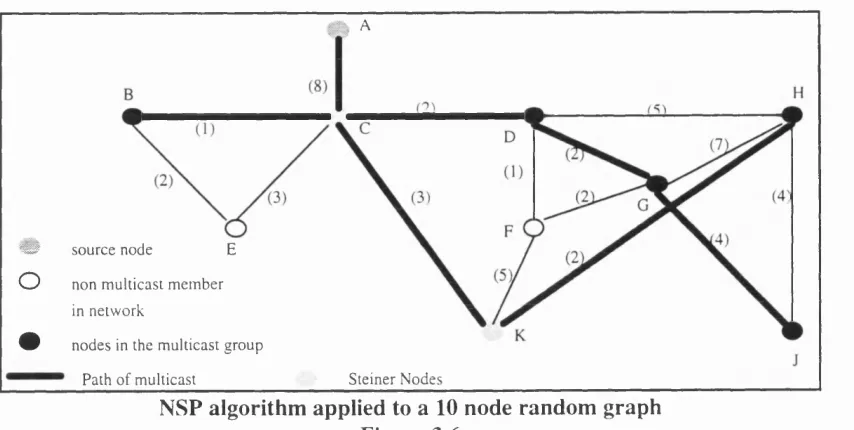
The source rooted shortest path (SP) algorithm, which uses multiple direct point-to-point connections with each of the destinations, the naive source rooted shortest path (NSP) algorithm [Doar_93a], which takes the union of the paths sharing a common link and the Greedy algorithm [Waxman_88], [Waxman_89] are also implemented. The performance of the GSDM routing algorithm is compared against the implementations of these dynamic multicast routing algorithms using randomly generated graphs to simulate the computer networks.

"Also, that the soul be without knowledge, it is not good; ... "

(4)

Preface

Except where otherwise stated in the text, this thesis is the result of my own work and is not the outcome of work done in collaboration. Furthermore, this thesis is not substantially the same as any I have submitted for a degree, diploma or other qualification at any other university. No part of this thesis has already been or is being concurrently submitted for any other degree, diploma or other qualification.

"If any o f you lack wisdom, let him ask o f God, that giveth to all men liberally, and

upbraideth not; and it shall be given him. "

James 1:5

Trademarks

UNIX is a trademark of AT&T.

(5)

Acknowledgements

I wish to thank my supervisor, Graham Knight, for the encouragement and valuable advice he gave me during the course of my research. I would also like to thank my second supervisor, Jon Crowcroft for his assistance and useful discussions during the course of my research. I would also like to thank the various members of the Computer Science Department, who have provided assistance and useful discussions during the course of my research, notably Ian Wakeman, Zheng Wang, Mark Handley and Tony Ballardie. Last but by no means least, I would like to thank my dearest friend, Simon D. Scott at Bath University, who has been a pillar of support and with whom I have had numerous discussions over the course of my research.

I am also indebted to the following people who have read and commented upon this thesis: Graham Knight, Jon Crowcroft, Zheng Wang and Simon D. Scott (Bath University). I am also grateful to all the wonderful people who shared the same office as myself over the three years that I have been at UCL, namely Miles Pebody, Tim Norman, Raghbir Sandhu, Lie Wang and Waleed El-Sonbaty, who have made my stay here, a pleasant and enjoyable one. I am also indebted to Robin Hirsch (UCL Computer Science Department) and Graham Bright well of the London School o f Economics for helping me with the complexity analysis.

I would also like to make a very special thanks to my whole family for the unwavering support they have given me throughout the period of my research. The last word of thanks goes to the fountain of all wisdom, the Lord Jesus Christ for his loving kindness.

"Jesus Christ the same yesterday, and today and forever"

Hebrews 13:8

(6)

Publications

1. M inimising Packet Copies in Multicast Routing by Exploiting Geographic Spread, ACM SIGCOMM Computer Communication Review, Volume 24, Number 3, July 1994, pages 47-62.

2. Exploiting Geographic Spread (GS) for Asynchronous Transfer Mode (ATM) Dynamic Multipoint Routing, the Fifth lEE Conference on “Telecommunications”, Brighton UK, 26-29 March, 1995, Publication Number 404, pages 262-267.

(7)

4 Geographic Spread... 66

4.1 Formal definition of Geographic Spread (G S )...67

4.2 Overview of the Geographic Spread Dynamic Multicast (GSDM) Routing Algorithm 68 4.3 Geographic Spread Dynamic Multicast (GSDM) Routing Algorithm... 70

4.3.1 Node A ddition...70

4.3.2 Node Rem oval...72

4.4 Network M odels...74

4.4.1 Random G raphs... 75

4.4.2 Hierarchical Random Graphs...78

4.4.3 Cost M etric...80

4.4.4 Simulation M odel... 81

4.4.5 Performance Evaluation Criteria... 81

4.4.5.1 Mean Inefficiency...82

4.4.5.2 The mean Packet C opies... 82

4.4.5.3 Computational Time Complexity...83

4.4.5.4 Scalability... 86

(10)

5 Performance Evaluation of the GSDM algorithm : Simulation

Results...

88

5.1 Simulation Environment...89

5.2 Performance of the GSDM algorithm for changing mean node degree: Simulation R esu lts... 93

5.3 Performance of the GSDM algorithm for a mean node degree of 3: Simulation R esu lts...101

5.4 The Effect of Hierarchical Graphs on the GSDM A lgorithm ...114

5.5 Sum m ary... 121

6 The Effect of Geographic Spread on Dynamic Multicast

Routing

:

Simulation Results

...125

6.1 GS T hreshold...125

6.2 Assessment of G S ... 125

6.3 Simulation R esults...126

6.3.1 How to control the GS of the resultant multicast trees...127

6.3.2 The Effect of GS on the GSDM algorithm ... 131

6.4 Sum m ary... 140

7 Comparison of Dynamic Multicast Routing Algorithms:

Simulation Results...

141

7.1 Simulation Results On Average Degree Random G raphs...142

7.1.1 Comparison results of the mean inefficiencies... 143

7.1.2 Comparison results of the mean packet copies... 149

7.1.3 Comparison results of the run time com plexities... 155

7.2 The Effect of Hierarchical Graphs on the SP, NSP, Greedy and GSDM routing algorithms... 163

(11)

7.2.2 Comparison results of the mean packet copies on hierarchical random graphs with

3 hierarchies...168

7.2.3 Comparison results of the run time complexities on hierarchical random graphs with 3 hierarchies...171

7.3 Sum m ary... 172

8 C o n c l u s i o n s ... 174

8.1 D iscussion... 174

8.2 Summary of Research Contributions... 180

8.2.1 Effect of Geographic Spread... 180

8.2.2 The Geographic Spread Dynamic M ulticast (GSDM) Routing Algorithm 181 8.2.3 Comparison of Dynamic Multicast Routing A lgorithms...181

8.3 Future W o rk...183

A : C a l c u l a t i o n o f G e o g r a p h i c S p r e a d ...185

B : S u m m a r y o f s o m e s t a t i s t i c a l m e a s u r e s ...191

B .l Standard Deviation (SD) a ...191

B.2 The Normal D istribution... 191

B.2.1 The Central Limit T heorem ... 192

B.2.2 The Shapiro-Wilk Test for N orm ality... 192

B.2.3 Statistical Inference... 194

B.2.3.1 Confidence Intervals... 194

B.2.3.2 Hypothesis Testing...195

C : A s y n c h r o n o u s T r a n s f e r M o d e : A n I n t r o d u c t i o n ... 198

C .l ATM C ells... 198

C.1.1 Cell Header Form at... 198

C.2 Advantages of ATM ...200

(12)

C.2.2 Non Hierarchical Multiplexing... 200

C.2.3 Fine Granularity Bandwidth Sharing... 201

C.2.4 Efficient Cell Switching... 201

C.2.5 Low and Bounded D elay... 201

C.2.6 Low and Predictable variation in delay (Jitter)... 202

C.3 Disadvantages of A T M ...202

C.4 ATM Protocol Reference Model (ATM _PRM )... 203

C.4.1 The Physical Layer... 204

C.4.2 The ATM L ayer...205

C.5 Relationship Between the B-ISDN and the O S IP R M ... 206

C.6 ATM Virtual Channels (VCs)...207

C .l ATM Virtual Path(s) (V Ps)... 208

C.7.1 Advantages of V Ps... 209

C.7.2 Disadvantages of VPs...210

C.8 ATM Adaptation Layer (AAL)... 210

C.8.1 Convergence Sublayer...211

C.8.2 Segmentation And Reassembly Sublayer... 211

C.8.3 The Adaptation Process... 211

C.8.4 AAL Service Applications... 212

(13)

List of Figures

Figure 2.1: Example of Time Division M ultiplexing... 14

Figure 2.2: Example ATM netw ork... 17

Figure 2.3: ATM Multicast Call Set-up E xam ple... 19

Figure 2.4: ATM Private Network Address Form ats... 21

F igure 2.5(a): Multicast Tree with minimum cost... 24

F igure 2.5(b): Multicast Tree with minimum delay...24

Figure 3.1: The KMB algorithm applied to a 9 node random graph ...40

Figure 3.2: The RS algorithm applied to an 8 node random grap h... 41

Figure 3.3: The Greedy algorithm applied to a 10 node g rap h... 48

Figure 3.4: The WGA applied to a 7 node graph... 49

F igure 3.5: SP algorithm applied to a 10 node random g ra p h ...50

Figure 3.6: NSP algorithm applied to a 10 node random graph... 52

F igure 3.7: Example of Distance Vector Truncated Broadcast deliv ery... 55

F igure 3.8: Multicast Tunelling... 63

Figure 4.0: Example of how to calculate G S ... 67

F igure 4.1: Example of local re-routing for adding a node to the multicast tr e e ... 69

F igure 4.2: GSDM routing algorithm applied to a 14 node random g ra p h ... 74

F igure 4.3(a): Waxman’s original 100 node random graph... 77

Figure 4.3(b): 100 node random graph with an average node degree of 3...77

F ig u re 4.4(a): Original 100 node hierarchical random graph with 4 hierarchies... 79

F ig u re 4.4(b): Hierarchical random graph with 4 hierarchies and an average node degree of 3 ... 79

F igure 5.1: GSDM’s number of nodes in the multicast group versus the number of modifications when 50% (i.e. 7^0.5) of the total nodes in the graph are in the multicast group for a 20 node random graph... 91

(14)

Figure 5.3; Mean inefficiency versus mean node degree for a 20 node graph with 50% of the total nodes in the multicast group...94

Figure 5.4: Mean packet copies per node versus the mean node degree for a 20 node graph with 50% of the total nodes in the multicast gro u p ... 95

Figure 5.5: Mean CPU time versus the mean node degree for a 20 node graph with 50% of the total nodes in the multicast group... 95

Figure 5.6: Mean nodes visited versus the mean node degree for a 20 node graph with 50% of the total nodes in the multicast group... 97

Figure 5.7: GSDM’s mean inefficiency versus the multicast group size for different mean node degree values for a 20 node g ra p h ... 98

Figure 5.8: Mean packet copies per node versus the multicast group size for different mean node degree values for a 20 node g ra p h ... 98

Figure 5.9: Mean CPU time (seconds) versus the multicast group size for different mean node degree values for a 20 node g ra p h ... 99

Figure 5.10: Mean nodes visited versus the multicast group size for different mean node degree values for a 20 node graph... 100

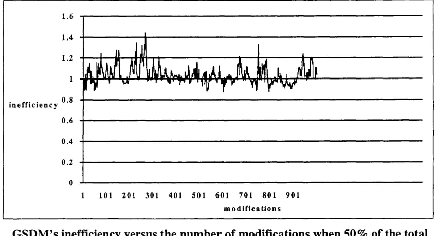
Figure 5.11: GSDM’s inefficiency versus the number of modifications when 50% of the total nodes in the graph are in the multicast group for a 20 node and a 100 node graph 101

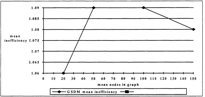
Figure 5.12: Mean inefficiency versus the number o f nodes in the graph when 50% of the total nodes in the graph are in the multicast group... 102

Figure 5.13: Standard deviation of mean inefficiency versus mean number of nodes in graph when 50% of the total nodes in the graph are in the multicast group...103

Figure 5.14: Mean inefficiency versus multicast group size for 20 and 50 node graphs 103

Figure 5.15: Mean packet copies per node versus the mean number of nodes in graph when 50% of the total nodes are in the multicast group...104

Figure 5.16: Standard deviation of mean packet copies per node versus mean number of nodes in graph when 50% of the total nodes in the graph are in the multicast group ..105

Figure 5.17: Mean packet copies per node versus multicast group size for 20 node and 50 node graphs versus the multicast group siz e ... 106

(15)

Figure 5.19: Mean CPU time (secs) per modification versus the multicast group size for 20 node and 50 node g rap h s... 108

Figure 5.20: Mean nodes visited per modification versus the mean number of nodes in the graph when 50% of the total nodes in the graph are in the multicast g ro u p 109

Figure 5.21: Ratio of KMB/GSDM mean nodes visited per modification versus the mean number of nodes in the graph when 50% of the total nodes in the graph are in the multicast group... 110

Figure 5.22: GSDM’s mean nodes visited per modification versus the (mean number o f

nodes in the graph f when 50% of the total nodes in the graph are in the multicast group

... I l l

Figure 5.23: KMB’s mean nodes visited per modification versus the (mean number o f

nodes in the graph f when 50% of the total nodes in the graph are in the multicast group

112

Figure 5.24: Mean nodes visited per modification versus the multicast group size for 20 node and 50 node graphs...113

Figure 5.25: Mean inefficiency versus the number of nodes in the hierarchical graph when 50% of the total nodes in the hierarchical graph are in the multicast group 114

Figure 5.26: Standard deviation of mean inefficiency versus mean number of nodes in the hierarchical graph when 50% of the total nodes in the hierarchical graph are in the multicast group...115

Figure 5.27: Mean packet copies per node versus the mean number of nodes in the hierarchical g ra p h ... 116

Figure 5.28: Standard deviation of mean packet copies per node versus mean number of nodes in hierarchical graph when 50% of the total nodes in the hierarchical graph are in the multicast group... 117

Figure 5.29: Mean CPU time (secs) per modification versus the number of nodes in the hierarchical graph when 50% of the total nodes in the hierarchical graph are in the multicast group... 118

(16)

Figure 6.1: Mean GS versus GS threshold for a 20 node random graph when 50% of the total nodes in the graph are in the multicast group... 127

Figure 6.2: Mean GS versus number of nodes in the multicast group for increasing GS threshold values for a 20 node random grap h... 127

Figure 6.3: Mean CPU time for a modification on a 20 node graph when 50% of the total nodes in the graph are in the multicast group... 129

Figure 6.4: Mean nodes visited versus GS threshold on a 20 node graph when 50% of the total nodes in the graph are in the multicast group... 130

Figure 6.5: Mean inefficiency versus mean GS for a 20 node graph when 50% of the total nodes in the graph are in the multicast group... 131

Figure 6.6: Mean packet copies per node versus GS threshold for a 20 node random graph when 50% of the total nodes in the graph are in the multicast group...132

Figure 6.7: Mean inefficiency versus multicast group size for different GS threshold values for a 20 node random g ra p h ... 133

Figure 6.8: Mean packet copies per node versus the multicast group size for different GS threshold values for a 20 node graph... 135

Figure 6.9: Mean CPU time (secs) per modification versus the multicast group size for different GS threshold values for a 20 node graph... 138

Figure 6.10: Mean nodes visited per modification versus the multicast group size for different GS threshold values for a 20 node graph... 139

Figure 7.1: Mean inefficiency versus the number o f nodes in the graph with 50% of the total nodes in the multicast g ro u p ...143

Figure 7.2: Standard deviation of mean inefficiency versus mean number of nodes in graph when 50% of the total nodes in the graph are in the multicast group...145

Figure 7.3: Mean inefficiency versus multicast group size for a 20 node g rap h 146

Figure 7.4: Mean inefficiency versus multicast group size for a 50 node g rap h 147

Figure 7.5: Mean packet copies per multicast tree versus the mean number o f nodes in the graph when 50% of the total nodes are in the multicast g ro u p ... 149

(17)

Figure 7.7: Mean packet copies per node versus the number of nodes in the graph when

50% of the total nodes in the graph are in the multicast group...151 Figure 7.8: Standard deviation of mean packet copies per node versus mean number of nodes in graph when 50% of the total nodes in the graph are in the multicast group ..151 Figure 7.9: Mean packet copies per multicast tree versus multicast group size for a 50

node graph...153

Figure 7.10: Mean packet copies per node versus multicast group size for a 50 node graph... 153

Figure 7.11: Mean nodes visited for a modification versus the mean number of nodes in the graph with 50% of the total nodes in the multicast group...155

Figure 7.12 Ratio of KMB/NSP and KMB/SP mean nodes visited per modification versus the mean number of nodes in the graph when 50% of the total nodes in the graph are in the multicast g ro u p ... 156

Figure 7.13 Ratio of KMB/GSDM and KMB/Greedy mean nodes visited per

modification versus the mean number of nodes in the graph when 50% of the total nodes in the graph are in the multicast g ro u p ... 156

Figure 7.14 GSDM’s, Greedy’s, NSP’s, and SP’s mean nodes visited p e r modification

versus the (mean number o f nodes in the graph f when 50% of the total nodes in the graph are in the multicast group...157

Figure 7.15 KMB’s mean nodes visited per modification versus the (mean number o f

nodes in the graph f when 50% of the total nodes in the graph are in the multicast

group... 158

Figure 7.16: Mean nodes visited per modification versus the multicast group size for a 20 node graph... 159

Figure 7.17: Mean nodes visited per modification versus the multicast group size for a 50 node graph...160

Figure 7.18: Mean CPU time per modification versus the mean number o f nodes in the graph with 50% of the total nodes in the multicast group... 161

Figure 7.19: Mean CPU time (secs) per modification versus the multicast group size for a 20 node graph... 161

(18)

Figure 7.21: Mean inefficiency versus the number of nodes in the hierarchical graph when 50% of the total nodes in the hierarchical graph are in the multicast g ro u p 164

Figure 7.22: Standard deviation of mean inefficiency versus mean number o f nodes in hierarchical graph when 50% of the total nodes in the hierarchical graph are in the

multicast group...165

Figure 7.23: Mean packet copies per multicast tree versus the mean number of nodes in the hierarchical graph when 50% of the total nodes in the hierarchical graph are in the multicast group...168

Figure 7.24: Standard deviation of mean packet copies per multicast tree versus mean number of nodes in hierarchical graph when 50% of the total nodes in the hierarchical graph are in the multicast group... 169

Figure 7.25: Mean packet copies per node versus the mean number of nodes in hierarchical g rap h... 169

Figure 7.26: Standard deviation of mean packet copies per node versus mean number of nodes in hierarchical graph when 50% of the total nodes in the hierarchical graph are in the multicast group... 170

Figure 7.27: Mean nodes visited per modification versus the mean number o f nodes in the hierarchical graph when 50% of the total nodes in the hierarchical graph are in the multicast group...171

Figure 8.1: A Multi-Core C B T ...184

Figure A l: Example Calculation of G S ... 185

Figure C .l: ATM Cell Format at the U N I... 199

Figure C.2: ATM Cell Format at the N N I... 199

Figure C.3: B-ISDN Protocol Reference Model (PRM )... 204

Figure C.4: Virtual Channel /Virtual Path Switching...208

(19)

List of Tables

Table 1.1: Characteristics of different applications which use multicast... 7

Table 3.1: The values of the function fi(v) for i g {%,2,3,4}... 41

Table 6.1: Mean GS and 95% GS confidence limits versus multicast group size for different GS threshold values for a 20 node g ra p h ...128

Table 6.2: Mean inefficiency and inefficiency confidence limits versus multicast group size for different GS threshold values for a 20 node graph... 134

Table 6.3: Mean packet copies per node and packet copies’ confidence limits versus multicast group size for different GS threshold values for a 20 node graph... 137

Table 7.1: Table of mean packet copies per node and mean packet copies’ confidence limits for increasing mean number of nodes in the graph with 50% of the total nodes in the multicast group...152

Table 7.2: Table of estimated worst case run time complexities of the GSDM, Greedy, NSP, and SP algorithms...158

Table 8.1: Table of mean inefficiencies for different multicast group sizes for the

GSDM, Greedy, NSP and SP algorithms for a 50 node g ra p h ... 176

Table 8.2: Table of mean packet copies per multicast tree and per node for different multicast group sizes for the GSDM, Greedy, NSP and SP algorithms for a 50 node graph...176

Table 8.3: Table of mean CPU time (seconds) for different multicast group sizes for the GSDM, Greedy, NSP and SP algorithms for a 50 node g ra p h ... 177

Table 8.4: Table of mean nodes visited for different multicast group sizes for the

GSDM, Greedy, NSP and SP algorithms for a 50 node g ra p h ... 178

Table 8.5: Table of mean inefficiencies for the GSDM, Greedy, NSP and SP algorithms for random and hierarchical random graphs as the size of the graph is increased 178

Table 8.6: Table of mean packet copies per node for the GSDM, Greedy, NSP and SP algorithms for random and hierarchical random graphs as the size of the graph is

increased...179

Table 8.7: Table of worst case run time complexities for the GSDM, Greedy, NSP and SP algorithm s...180

(20)

Glossary of Terms

The following abbreviations are frequently used in this thesis. Where appropriate, they are explained in greater detail when they first appear in the text.

AAL

ATM

Broadband

B-ISDN CAC

Call

CATV CCITT

Connection

End System

Asynchronous transfer mode Adaptation Layer - highest layer of the ATM Layered Model.

Asynchronous transfer mode, a specific packet oriented transfer mode using an asynchronous time division multiplexing technique that allows multiple logical connections to be multiplexed over a single interface.

A service or system requiring transmission channels capable of supporting rates greater than the Integrated Services Digital Network primary rate i.e. bit rates in excess of 2 Mbits/s.

Broadband Integrated Services Digital Network.

Call Admission Control. The procedure used to decide if a request for an ATM connection can be accepted based on the attributes of both the requested connection and the existing connections.

A call is an association between two or more users or between a user and a network entity that is established by the use of network

capabilities. This association may have zero or more connections. Community Antenna Television.

The International Telegraph and Telephone Consultatative Committee (Comite Consultatif International de Télégraphique et Téléphonique). This has now been renamed the International Telecommunications Union - Telecommunications Sector (ITU-T).

An ATM connection consists of the concatenation of ATM Layer links in order to provide information transfer capability of access points.

(21)

GS

HDTV

HEC HOL IGMP

Internet IP

ISDN

ISO

Isochronous LAN

MAC

Geographic Spread. Given a graph G=(V,E), where V is the set of vertices and E is the set of edges and a subset C/çV the geographic spread of the set (/, in the static case when tree T spans U is defined as the inverse sum of the minimum distance from a vertex v to a vertex in T , over all vertices ve V.

High Definition Television - 1920x1035 pixel resolution (American) compared to 768x576 for ordinary UK television.

Header Error Check - error detection/correction on a cell header. Head Of Line - head of a queuing system.

Internet Group Management Protocol - the protocol implemented in hosts and routers on LANs to monitor multicast group presence on a subnetwork.

A collection o f interconnected networks.

Internet Protocol - the (TCP/IP) protocol that formally specifies the format of Internet packets (datagrams), routing, error handling, etc. and provides connectionless network service between multiple packet switched networks interconnected by gateways.

Integrated Services Digital Network - an all digital network in which all source information is transmitted and switched as digital signals end to end and this allows a common signal transfer mechanism to be employed in the network to serve several applications that are quite different in nature , e.g. voice and data transmission.

International Standards Organisation.

Traffic repeating in time such as 8kHz voice samples.

A data communications network used to interconnect a community of digital devices distributed over a localised area of up to about lOkm^. The devices may be office workstations, mini-computers, etc.

Medium Access Control - a procedure used by each device in a shared transmission medium to ensure that transmissions occur in a

(22)

MAN

MID

Multiplexer

MST

NNI OAM

Optic Fibre

OSI PDU

Plesiochronous Primitive

Protocol

PTM PVC QOS

RFC

Metropolitan Area Network - a data communications network that links a set of LANs that are physically distributed around a town or city.

Multiplexing IDentifier - an identifier to say from which source information came.

A device used to enable a number of lower bit rate devices, normally situated in the same location, to share a single higher bit rate

transmission line.

Minimum spanning tree - is a collection of edges connecting all the vertices such that the sum of the weights of the edges is at least as small as the sum of the weights of any other collection of edges connecting all the vertices.

Network Node Interface - internal interface within B-ISDN.

Operations, Administration and Maintenance - gathering and reporting of network statistics.

A transmission medium over which data is transmitted in the form of light waves or pulses. It is characterised by its potentially high bandwidth, data carrying capacity and its high immunity from interference from other electrical sources.

Open Systems Interconnection.

Protocol Data Unit - a unit of information in a communications protocol, together with the protocol overhead.

Variable frequency traffic such as compressed video.

An abstract, implementation independent, interaction between a layer service user and a layer service provider.

A set of rules and formats (semantic and syntactic) formulated to control the exchange of data between two communicating parties. Packet Transfer Mode.

Permanent Virtual Connection.

Quality of Service - the standard demanded of a transmission channel in a network.

(23)

R outer

SAR

SDH

SDU

SMDS

SM T

STM STP SVC UNI

vc

vcc

V CI

VCL

VP VPC

A device used to interconnect two or more LANs together, each of which operates with a different MAC protocol.

Segmentation and Reassembly - the breaking up of packets into smaller data units and their reassembly again.

Synchronous Digital Hierarchy - a CCITT defined set o f data rates and switching system which allows payloads to be added and extracted without unpacking the entire data structure.

Service Data Unit - a unit of information in a communications protocol without the protocol overhead of that layer.

Switched Multi-megabit Data Service - a connectionless MAN inter networking scheme.

Steiner Minimal Tree - the minimal cost subgraph (tree) spanning a given subset of nodes in a graph.

Synchronous Transfer Mode. Steiner Tree Problem in graphs. Switched Virtual Connection.

User Network Interface - interface from B-ISDN to an external device.

Virtual channel - a communication channel that provides for the sequential unidirectional transport of ATM cells.

Virtual channel connection - a concatenation of VC links that extends between the point where the ATM service users access the ATM Layer.

Virtual Channel Identifier - a connection identifier in an ATM network.

Virtual channel link - a means of unidirectional transport of ATM cells between the points where a VCI value is assigned and the point where that value is translated or removed.

A bundle of VCs.

(24)

VPI Virtual Path Identifier - an identifier for a group o f virtual channels in an ATM network.

(25)

Chapter 1 Introduction

It is now widely accepted that the Asynchronous Transfer Mode (ATM) technique will be the switching and multiplexing technique for future broadband networks [Cox], [Ammar],

Multicast communication will play a critical role in future broadband computer networks, such as high-definition television distribution and multimedia conferencing [Kompella_93], [Kadirire_95b]. Multicast can be defined, loosely, as the ability to logically connect a subset of the hosts in a network. The number o f sources and destinations can be one each, in which case the connection is referred to as 'point-to- point' or 'unicast', or all the hosts in a network, in which case the connection is referred to as 'broadcast', or there may be any numbers in between [Doar_93a]. A packet switched network is said to provide a multicast service if it can deliver a packet to a set of destinations or a ‘multicast group’, rather than to just a single destination. A ‘multicast group’ is a collection of hosts that are the destinations of the same set of messages [Frank], [Garcia-Molina]. These messages may originate at one or more source sites and the destination hosts may run on one or more sites, not necessarily distinct.

(26)

provide its own ad hoc solution to a number of complex problems resulting in inefficient use of the network resources.

A good overview of routing in high speed networks is given by Ren-Hung Hwang [Hwang] in his Ph.D. thesis. A routing algorithm in a computer network has two essential functions, i.e. the selection of routes for various origin-destination pairs and the delivery of messages to their correct destinations. The problem of routing connections in broadcast or multicast networks is quite different from routing in point-to-point networks. A point-to-point network can be described as a graph in which each edge has a capacity and a length [Waxman_88]. A set of connections for such a network is simply a collection of vertex pairs. A feasible route assignment is an assignment of each connection to a path in the network joining the connection's endpoints that does not exceed the capacity of any edge, i.e. the number o f connections using any particular edge must be bounded by the capacity of that edge. An optimal routing algorithm is one that can find a feasible assignment (route) whenever one exists and also performs optimal assignment of traffic to routes; which can be regarded as similar to the goal of link sharing versus delay based optimal multicast routes in some sense.

The multicast routing problem can be modelled in a similar way. With multicast routing, one is interested in the shortest (minimum cost spanning) subtree of the network containing a given set of hosts (i.e. the multicast group). One is not only interested in finding this minimum spanning tree, but also in minimising the cost of the routing calculations i.e. minimising the time complexity o f the routing algorithm. The multicast routing problem is the problem of finding such a subtree and the intuitive interpretation of a routing tree is that the source node sends a copy of the message which is transmitted down the branches of the subtree until all nodes in the tree have a copy of the message [Tanaka_93]. This is essentially a Steiner Tree problem (STP) in graphs and is known to be NP-complete [Karp]. A problem in the class NP is said to be

NP-complete if it has the property that if a polynomial time algorithm can be found to

solve it (i.e. if the problem is shown to be in the class P), then P=NP. In other words,

the NP-complete problems are those which are in some sense the ‘hardest’ problems in

the class NP. (For a formal definition of the multicast routing problem, see chapter 2).

(27)

like asynchronous transfer mode (ATM) networks. Dynamic in this case is used to mean that nodes which are already in the multicast group may leave or nodes which are not in the multicast group may join at any time during the lifetime of the multicast group.

1.1 Uses of Multicast

A multicast service can offer several benefits to network applications, some o f which are listed below:

1.1.1 Efficient multi-destination delivery

When an application must send the same information to more than one destination, multicasting is more efficient than unicasting separate copies to each destination. It reduces the transmission overhead on the sender and it can also reduce the overhead on the network and the time taken for all destinations to receive all the information. Examples of applications that can take advantage of multi-destination delivery are [Deering_91] :

• updating all copies of a replicated file or database;

• sending multimedia traffic (e.g. voice, video, or data packets) to all participants in a computer mediated conference;

• distributing intermediate results to a set of processors supporting a distributed computation.

1.1.2 Logical addressing

If a set o f destinations can be identified by a single group address (rather than by a list of individual addresses), such a group address can be used to reach one or more destinations whose individual addresses are unknown to the sender, or whose addresses may change over time. Sometimes called logical addressing or location-independent addressing, this use of multicast serves as a simple, robust alternative to configuration files, directory servers, or other binding mechanisms. Examples o f applications that can take advantage of logical addressing are:

(28)

• locating an instance of a particular network service, such as name service or bootstrap service.

• sending sensor readings or status reports to a self-selected, changeable set of monitoring stations. This is an example of an application that exploits both the logical addressing and the multi-destination delivery of multicast [Deering_91].

1.1.3 Conferencing

Any form of conferencing (e.g. audio, video or shared data) can benefit from using multicast when the number of destinations is small, as well as large. Conventional voice conversations are not particularly useful with multiple participants, mainly due to the lack o f co-ordinating signals, but multiple party video telephony can be made to work well and promises great reductions in the cost o f travelling to meetings. One instance of data conferencing where the multicast group size is small, that would benefit from the provision of multicast in a network is the 'virtual white board' application, where all participants can see what is being drawn on a screen and may be able to modify the screen themselves. An example o f a large, high occupancy multicast group, for the conferencing service, might be some form of computer conferencing, where parallel distributed machines constantly update each other with information. For all forms of conferencing, it must be possible to add members to the multicast group, delete them from the group, establish sub-groups within the group and to merge groups together during the conference i.e. after data has been sent by some participants.

1.1.4 Wide-scale distribution

(29)

distribution of an important event like the football world cup where perhaps even up to 90% of the viewers (hosts) tune in.

1.1.5 Distance learning

Distance learning, with a lecture being transmitted directly to a small group who are interested, rather than to the whole nation. This will involve the interactive distribution of text, sound and images from learning centres to a wide variety of locations. A system for distance learning called Theseus, was developed at John Moores University, which pulls together the multimedia environment required for distance learning, for presentation to the student on a single PC screen as part of the Super JANET project [Head], [Clyne].

1.2 Broadband ATM Services and Applications

There is an emerging demand for broadband services that require transmission bandwidth with more than 150 Mbits/s, as well as high speed switching and processing. This can be realised by constructing the broadband integrated services digital network (B-ISDN) using asynchronous transfer mode (ATM) technology [Handel], [De Prycker]. The International Telegraph and Telephone Consultative Committee (CCITT), now known as the International Telecommunications Union - Telecommunications Sector (ITU-T), defines B-ISDN as "a service requiring transmission channels capable

o f supporting rates greater than the prim ary rate" [Stallings_95] (page 408). This

(30)

networked computing and user friendly graphical interfaces and the convergence of telecommunications and computing is accelerating the demand for broadband services. In some countries like the USA, the Federal Communications Commission has recommended the elimination of telephone company and cable television (CATV) company cross-ownership restrictions. This invariably allows competition between the local exchange carriers or network operators and the CATV companies to expand into each other’s former businesses [DeMaio]. Consumer demands for broadband services may be dramatically altered by a number of economic, social and lifestyle changes. Transportation costs continue to rise and a growing number of employees are opting for work at home arrangements (telecommuting) and flexible time work schedules.

An extremely wide range of services is expected to be offered over an ATM based network, for example:

1.2.1 High Speed Image Networking Service

This service is likely to have applications like:

• design automation using computer aided design and computer aided manufacturing, • medical imaging and consultation,

• photographic editing, scientific visualisation and high-resolution graphics and image rendering.

1.2.2 Interactive Multimedia Service

This service is likely to support business applications like: • interactive tele-training,

• telecommuting/work-from-home, • print/publishing collaboration,

• virtual reality, in which the application gives the user the illusion of being in another place [Partridge].

• subject matter expert consultation, • multimedia telephony and

• multimedia conferencing in which participants can use their multimedia workstations (computers) to see and talk to each other.

(31)

• multimedia electronic mail,

• interactive multimedia distance learning, • multimedia videotext/‘yellow pages’ and • interactive television and games.

1.2.3 Broadband Distribution Video Service

This is likely to support residential applications like:

• broadcast television/high definition television distribution (HDTV), • broadcast distance learning,

• video on demand and

• video catalogue/advertising and tele-shopping.

1.2.4 Wide-area Network Distributed Computing Service

This is likely to support applications like:

• local area network (LAN) backbone/interconnect, host to host channel networking and load sharing [DeMaio].

Application Total hosts in network

Multicast size

Bandwidth (bits/s)

Burstin ess

Static/Dy namic Distributed

database

10-100 1-10 1.5-130M 1-50 Static

Service Location > 100 > 100 < 100K Static Audio Conference 10-100 1-10 32K 2 Dynamic Video Conference 10-100 1-10 1.5-130M 1-5 Dynamic

Whiteboard 10-100 1-10 IK -IM Dynamic

Audio distribution >100 >100 1-2M Dynamic Standard quality

video distribution

>100 >100 1.5-15M 2-3 Dynamic

HDTV distribution >100 >100 15-150M 1-2 Dynamic

Characteristics of different applications which use multicast Table 1.1

Table 1.1, which was compiled from [Handel], [Huber] and [Doar_93a] shows the different characteristics of the various applications, some of which have been outlined above, that use multicast. The bandwidth quoted is the mean bit rate and the burstiness

(32)

to applications which will need the whole destination set to be known before the multicast connection is set-up i.e. static, or applications which can join or leave a multicast session at any time during the lifetime of that session i.e.dynamic. This essentially means that the broadband network platform must be service independent and for efficient network utilisation, most o f these applications that have been described above will need to be multicast.

1.3 Research Aims

There are essentially three main aims to this research i.e.

• Identifying the problem of Geographic Spread (GS) i.e. the concept of spreading out the multicast connections geographically within the network so that with time, as nodes join the multicast group, the probability of a node being geographically close to the multicast connection is high [Kadirire_94], A formal definition of GS is given in chapter 4. Investigating how GS can be used to help solve the problem of

dynamic multicast routing in wide-area packet switched communications networks

like Asynchronous Transfer Mode (ATM) networks.

• Investigating dynamic multicast routing algorithms in wide-area ATM communications networks. Investigations of some of the more popular current dynamic routing algorithms proposed in the literature for multicast (point-to- multipoint) communications are carried out. The thesis reveals the short-comings of these algorithms and hence justifies the need for more research into dynamic multicast routing algorithms. The thesis investigates how better dynamic multicast routing algorithms can be developed drawing on the experiences o f algorithms like the source rooted Shortest Path (SP) algorithm, the naive source rooted Shortest Path (NSP) algorithm, [Doar_93a], and the Greedy algorithm [Waxman_88].

(33)

connection*, it just adds a node via the nearest path to the connection and does not try to consider the long term effects of this, nor does it consider how this greedy approach affects the rest of the multicast connection from a global view point. A new dynamic multicast (point-to-multipoint) routing algorithm for ATM networks, called the ‘Geographic Spread Dynamic M ulticast' (GSDM) [Kadirire_94] routing algorithm is proposed and implemented. The GSDM routing algorithm looks at the problem of routing multicast connections globally by spreading out the connections ‘geographically’ when applying the ‘Geographic Spread’ criteria for choosing a path to add a node to the multicast connection. At the same time it adds a node to the multicast connection using local optimisation o f the multicast connection. It incorporates some aspects of the SP/NSP algorithm to keep the time complexity down. It also adopts the approach taken by the Greedy algorithm of finding the nearest path from the node that wants to join the multicast group, but also considers other paths. In considering other paths, it employs GS to make sure that not only local optimisations (choosing the ‘best’ path to add a node to the multicast connection) are achieved, but the whole network benefits in the long term.

Multiple simulations" are performed to test the performance of the GSDM routing algorithm against the implementation of a well-known near optimal Steiner tree heuristic commonly referred to as the KMB algorithm [Kou] in the literature. The SP, the NSP and the Greedy algorithm are also implemented and the performance of the GSDM routing algorithm is compared against these in terms of the number of packet copies per node, the delay i.e. the time taken to add or remove a node to or from the multicast group, the mean number of nodes visited when computing the cost of the multicast tree and the inefficiency, using the KMB algorithm as a basis on which to measure the

inefficiency of the algorithms. Inefficiency is defined as the ratio of the cost of the

multicast tree generated by an algorithm for a given set o f nodes in the multicast group, to the cost of the tree for the same nodes in the multicast group, generated by the KMB algorithm, a near optimal Steiner tree heuristic [Doar_93a]. The effect of GS on the

* M u ltica st con n ection and m u lticast tree are u sed in terch a n g ea b ly and m ean the sa m e thing in this thesis

(34)

GSDM routing algorithm is investigated to see how performance parameters like the delay, number of packet copies per node, inefficiency and scalability (i.e. performance as the number of nodes in the multicast group is increased from 10% to 80% o f the total nodes in the graph) are affected.

1.4 Assumptions

The following assumptions have been made in this thesis: • All the ATM switches (nodes) have multicast capability; • There are no link or node failures;

• The thesis only deals with the routing strategy and assumes that there is a perfect underlying system in place which manages the routing tables and also takes care of any cell re-ordering problems which might be caused by re-routing connections. Although one does not consider the possible problem of cell re-ordering because of re-routing some connections, it has been shown by Cohen [Cohen_94a], Cohen and Segall [Cohen_94b] and by Anderson et. al., [Anderson] that connections can be intentionally re-routed in ATM networks without incurring cell re-ordering or generating duplicate cells.

• Virtual Path (VP) routing is assumed, where a VP is a direct logical connection between two ATM switches with some assigned capacity. Typically, each node, while not physically connected to all the other nodes in the network, has an assigned VP to every other node in the network [Ammar]. Assuming that there is only one VP between a pair of nodes, in a fully connected ATM network with N nodes, there will be VPs.

2

1.5 Thesis Outline

(35)

(36)

1.6 Summary

(37)

Chapter 2 Asynchronous Transfer Mode (ATM) and

Multicasting

The term ‘transfer m ode’ is used by the CCITT to describe a technique used in a telecommunications network, covering aspects relating to transmission, multiplexing and switching [De Prycker], [Handel]. In this chapter, a brief overview of the ATM technology, including signalling, addressing, point-to-point and point-to-multipoint routing is given. A formal definition of the static and dynamic multicast routing problem is also given and some of the problems of multicasting in ATM networks are outlined.

2.1 Synchronous Transfer Mode (STM)

In digital circuit-switched networks, the sub-channels representing instances of concurrent communication are multiplexed together by synchronous time division multiplexing. Suppose the transmission line has a capacity C bits per second, then the

C

transmission line's capacity can be shared by at most N = — transmitting terminals, X

where X is the terminal transmission bit rate. The (infinite) time horizon can be marked into intervals of some convenient duration, 6 as in figure 2.1 below and each interval is called a time frame [Hui],[De Prycker]. The interval Ô may be chosen as follows: if one takes for example, the telephone network in which the voice signals are sampled at 8000

times per second, 5 would be ^ sec = 125 jisec. Each frame is divided into N time

oOOO

5 5

slots of equal duration — , during which n = C x — bits can be transmitted. A terminal

N N

(38)

Single Slot Time Division Multiplexing (TDM)

1 time friime = 5 seconds V.

N N-1 N-2 4 3 2 1

V —

Example of Time Division Multiplexing Figure 2.1

2.1.1 Integrated Services Digital Network (ISDN)

Integrated broadband networks are being conceived as an extension of 64k bits/s based integrated services digital networks (ISDN). ISDN is an all digital network in which all source information is transmitted and switched as digital signals end-to-end and this allows a common signal transfer mechanism to be employed in the network to serve several applications that are quite different in nature, e.g. voice and data transmission. CCITT defined ISDN as "a network .... that provides end-to-end digital connectivity to support a wide range o f services, including voice and non-voice services, to which

users have access by a limited set o f standard multi-purpose user-network interfaces”.

One such interface is called the ‘basic access’, comprising two 64 Kbits/s channels, called the B channels and a 16 Kbits/s signalling channel called the D channel. Another type of interface, the ‘primary rate access’, has a gross bit rate of 1.544 Mbits/s for the United States of America, Japan and Canada and a gross bit rate of 2.048 Mbits/s for the European countries. Typically, the channel structure for the 1.544 Mbits/s rate will be 23 B channels plus one 64 Kbit/s D channel and, for the 2.048 Mbits/s rate, 30 B

channels plus one 64 Kbits/s D channel. Channel 32 provides framing and management bits. The primary rate access offers the flexibility to allocate high speed primary rate channels or H channels or mixes of B and H channels, and a 64 Kbits/s signalling D

(39)

This mode of operation is referred to by the CCITT as synchronous transfer mode (STM) [McAuiey], and it has the advantage that the switching mechanisms are comparatively straightforward and switches can be implemented in hardware to provide a very high aggregate bandwidth. The hardware for the user equipment for a STM network is also simple as it can be connected to the network by synchronising it to the network clock. The ISDN design achieves a substantial degree of network integration, but little in the way of service integration. The advantage of ISDN over current packet switched networks or separate voice networks is better file transfer, plus a competitive advantage to telephone companies. However, large file and image transfer is still inconveniently slow and good quality video is not feasible, e.g. a 10^ bit high resolution image takes over 4 hours at 64 Kbits/s access and 11 minutes at 1.5 Mbits/s access.

2.2 Packet Transfer Mode (PTM)

In packet switched networks, the sub-channels are multiplexed by asynchronous time division multiplexing and the term asynchronous applies to the channel access mode. There are several medium access control protocols (MACs) like ‘token passing ’ used in a Token Ring local area network (LAN) topology, ‘queued-packet, distributed-switch'

(QPSX) [Halsall], used in a distributed-queue dual-bus (DQDB) high-speed broadcast metropolitan area network (MAN) for connecting LANs and the ‘carrier sense multiple

access with collision detection ’ (CSMA/CD) used in shared bus network topologies like

(40)

The addressing information present in each packet can be either global or relative to some shared context between nodes. The network is then said to be based on either

‘datagram s’ or ‘virtual circuits’, respectively. The benefit of relative addresses is that

they are substantially smaller than global addresses and so use a smaller proportion of the available bandwidth and can be used for direct hardware lookup for routing functions. The disadvantage of relative addressing is that it requires an association set up stage to pass the mapping between global and relative addresses to all involved switching nodes. Due to the presence of an association set-up phase, these networks are referred to as virtual circuit networks. The advantage of global addressing networks, i.e. those based on datagrams, is that they do not require any association set-up mechanism. However, this is at the cost of a more expensive switching mechanism per packet. This asynchronous mode of operation, of both datagram and virtual circuit networks, is referred to by the CCITT as packet transfer mode (PTM) [McAuley]. The main advantage of PTM is that two communicating entities have the possibility of utilising all of the available bandwidth between the two nodes. Also, the traffic generated by computers tends to be of a bursty nature and so is well suited to PTM networks. Not all PTM systems incur contention which needs resolving e.g. ‘Token R ing’ networks which control access by ‘token passing’. However, the main disadvantage of PTM in a shared bus network like Ethernet, is that the use of a contention resolution mechanism always introduces variability in the delay or jitter, associated with access to the channel and this may not meet the stringent delay requirements needed for some services.

2.3 Asynchronous Transfer Mode (ATM)

(41)

transfer mode in which information is organised into cells; it is asynchronous in the

sense that the recurrence o f cells containing information from a particular user is not

necessarily periodic”

S o u r c e A (V o ic e )

S3 b y t e c e il ATM SWITCH/

m u l t ip l e x e r

JU L U

(V id e o )

ATM SWITCH

Hign s p e e d link (1 5 5 /6 2 2 M b /s)

S o u r c e C (file tra n sfe r)

S o u r c e 0 (G ra p h ic s )

Example ATM network Figure 2.2

It represents a compromise between the multiplexing mechanisms of STM and PTM

[McAuley]. The channel is slotted into fixed intervals of duration — , where Cs is the

Lc

(42)

2.4 ATM signalling

ATM signalling protocols vary according to the type of ATM link being used i.e. ATM

‘user network interface ' (UNI) signalling is used between an ATM end-system and an

ATM switch across an ATM UNI and ATM ‘network node interface’ (NNI) signalling is used across NNI links. The current standard o f ATM UNI signalling is described in the ATM Forum UNI 3.0/3.1 [ATM Forum], and work is still continuing on the NNI signalling. ATM signalling uses the ‘one-pass’ method of connection set-up, which is the model used in all common telecommunications networks e.g. the telephone network [Allés]. A source end-system wishing to set-up a call will formulate a SET-UP message containing the destination end-system address, desired traffic and QOS parameters. This set-up message is sent to the first ingress switch across the UNI which responds with a local CALL PROCESSING acknowledgement. The ingress switch then invokes an ATM routing protocol which propagates the signalling request through the network, setting up the connection as it goes until it reaches the final destination end-system. The routing of the connection request and hence of any subsequent data flow, is governed by the ATM routing protocol, which routes the connection request based upon both the destination address and the traffic and QOS parameters requested by the source end- system. The egress switch on the other end will then forward the set-up message to the end-system across its UNI, which may choose to either accept or reject the connection request [McDysan]. If it accepts the connection request, it sends a CONNECT message back to the source end-system along the same path and, once the source end-system receives this CONNECT message, either node can start transmitting data on the connection. If, on the other hand, the destination end-system rejects the connection request, it returns a RELEASE message which is also sent back to the source end- system, clearing any allocated resources as it proceeds.

(43)

a t m sw itch C aJling P a n y NihJc A

ATM N etw ork

. T i t ,

Leal NixJc C :a l lp r o c e e d i n g

:O N N E C T C O N N E C T

C O N N E C T ACK ■A RTY C

ID PARTY ACK C ADD PA RTY A C K C

S E T L T to D AD D PARTY D

C O N N E C T

CO N N E C T ACK

AD D PA RTY ACK D

ATM M ulticast Call Set-up Example Figure 2.3

Figure 2.3 shows an example of setting up a multicast- call from the source (originator

or root) node A to tw o other nodes which wish to join the m ulticast group, node B and

node C connected to a local ATM switch and node D, connected to a separate ATM

UN I [M cD ysan], [ATM Forum ]. N ode A initiates the m ulticast call by sending a S E T

U P m essage to the ATM netw ork, requesting a m ulticast call to be set-up, identifying

leaf node B ’s ATM address. The netw ork responds with a C A LL PR O C E SSIN G

m essage and routes the call using an appropriate point-to-m ultipoint routing algorithm

(e.g. the G SD M algorithm ) to the physical interface on which node B is connected. It

then issues a SE T -U P message to node B, identifying the assigned V PI/V C I should the

call be accepted. The first leaf node (node B) then indicates its intention to join the call

by returning a C O N N EC T m essage, to which the netw ork acknow ledges with a

C O N N E C T A C K N O W LED G E message. The netw ork then informs the source node A

o f a successful addition o f node B via a C O N N E C T and a C O N N E C T

A C K N O W L E D G E handshake as shown in the figure 2.3. T he source node then requests

that node C be added to the m ulticast connection through the A D D PA R T Y m essage,

which the netw ork routes to the same ATM UN I as node B via the A D D PA RTY

m essage to inform the local ATM switch o f the requested addition. N ode C then

responds with an AD D PA RTY A C K N O W LED G E m essage that is sent by the netw ork

back to the source node A. The source node A then requests that the final party, node D

(44)

be added to the multicast connection via the ADD PARTY message again. The network then routes this call to the UNI connected to node D and issues a SET-UP message since this is the first party on this ATM UNI. Node D then responds with a CONNECT message to which the network responds with a CONNECT ACKNOWLEDGE message. The fact that node D has joined the multicast call is conveyed back to the source node A via the ADD PARTY ACKNOWLEDGE message. The leaves of the point-to-multipoint call may be removed from the call by the DROP PARTY message if one or more hosts or parties would remain on the call on the same UNI, or by the RELEASE message if the party is the last leaf on the same UNI. The source node should drop each node in turn and then release the entire connection.

2.5 ATM addressing

The ITU-T has settled for the telephone-number-like (CCITT Recommendation E.164) [Bubenik_92] addresses as the addressing structure for public ATM (B-ISDN) networks and the ATM Forum has extended ATM addressing to include private networks. The addressing scheme chosen by the ATM Forum [ATM Forum] for use with UNI 3.0/3.1 signalling, is known as the ‘subnetwork’ or ‘overlay’ model which works the same way as protocols like IP over X.25 [McDysan], [Alles]. All protocols operating over an ATM subnetwork will require some form of ATM address resolution protocol (ARP) as proposed by Mark Laubach in RFC 1577 [Laubach] and Grenville J. Armitage [Armitage_95] to map higher layer addresses (e.g. IP addresses) to their corresponding ATM addresses.

Dynamic multicast routing in the Asynchronous Transfer Mode environment