An Improved Hydrodynamics Formulation for Multiphase Flow Lattice-Boltzmann Models

+Dept. of Mechanical Engineering, National Technical University of Athens, Greece

Lattice Boltzmann (LB) models provide a systematic formulation of effective-field computational approaches to the calculation of multiphase flow by replacing the mathematical surface of separation between the vapor and liquid with a thin transition region, across which all magnitudes change continuously. Many existing multiphase models of this sort do not satisfy the rigorous hydrodynamic constitutive laws. Here, we extend the two-dimensional, seven-speed Swift et al LB model1 to rectangular grids (nine speeds) by using symbolic manipulation (Mathematica) and comparing the LB model predictions with benchmark problems, in order to evaluate its merits. Particular emphasis is placed on the stress tensor formulation. Comparison with the two-phase analogue of the Couette flow and with a flow involving shear and advection of a droplet surrounded by its vapor reveals that additional terms have to be introduced in the definition of the stress tensor in order to satisfy the Navier-Stokes equation in regions of high density gradients. The use of Mathematica obviates many of the difficulties with the calculations "by-hand", allowing at the same time more flexibility to the computational analyst to experiment with geometrical and physical parameters of the formulation.

1. Introduction

Coarse-grained (mesoscopic) models of multi-component fluid flow and phase change constitute an intermediate step towards engineering design of thermo-fluid systems, situated between molecular dynamics and Navier-Stokes models. Lattice Boltzmann (LB) methods, which are based on a broad class of such discrete models, share the physical resolution of the microscopic and the economy of the macroscopic worlds, and provide a convenient way to incorporate complex interfacial physics in an ab-initio fashion. Although already popular in condensed matter physics, these methods are slowly being introduced in the study of problems on the scale of gas-liquid interface width, cf. Chen2 , Shan3, and He4. Direct-simulation Monte-Carlo, another coarse-grained modeling technique, was recently extended by Carey and Hawks5 to model evaporation of microdroplets.

In addition to incorporating correct physics, accuracy is of paramount importance in predictive simulations. LB methods have been proven to be equivalent to second-order finite-difference approximations of Navier-Stokes flows in complex domains, cf. Noble et al6. In addition to high numerical efficiency owing to parallelization, LB methods can accommodate complex interfacial physics while still allowing time integration on the scale of mean-free time-which is two orders of magnitude faster than what molecular dynamics methods allow. Two recent schemes have been reported for two-dimensional two-phase flows: Swift et al1 simulated gas-liquid interfaces of a van der Waals fluid with a LB model, while Jasnow and Vinals7 simulated thermo-capillary induced flows by coupling the Cahn-Hilliard with the extended Navier-Stokes equations. In order to explore the first scheme further, the LB scheme is revisited here by performing the formulation steps via symbolic computation, isolating the truncation error, and assessing the importance of this error by comparing with limiting two-phase flows.

2. Method

LB models are based on calculating the probability distribution f_σi( , )x t , which is associated with the probability that a particle at location x and time t is moving with velocity eσiα. The velocity

square lattice assumes values of 0 for stationary, 1 for vectors aligned with the Cartesian axes, and 2 for diagonal vectors. The i subscript denotes the specific direction of each vector ranging from 1 to 4 for the two non-zero velocity classes, and the α subscript denotes the vector components. To obtain physical quantities, statistical mechanics concepts are employed. The density ρ and velocity vector u_α are determined by evaluating moments of the probability distribution

ρ = _σ

σ, f _i

i

∑

ρuα=

∑

i

σ σ α σ,

e (2)

Once these macroscopic quantities are evaluated, an evolution step is carried out using the lattice Boltzmann evolution equation

f_σi(x +

e_σi

c x

α _{∆ ,t + ∆t) − f}

σi(x, t ) = − −

1 0

τ(fσi fσi) (3)

where fσi 0

is the equilibrium distribution, ∆t the time step, ∆x the lattice spacing, c the computational speed of sound (∆x/∆t), and τ a non-dimensional relaxation time which dictates the rate at which the system decays toward equilibrium relative to the time step. After the collision, the modified distributions advance to other neighboring sites (advection step).

As the Boltzmann evolution equation suggests, the form of the equilibrium distribution governs the macroscopic evolution process. To determine the equilibrium distribution for the square lattice two-phase using Swift’s model, a general form is initially assumed.

fσi 0 _{= Α}

σ + Βσeσiαuα+ Cσu2 + Dσeσ α σ β α βi e i u u + Gσαβeσ α σ βi e i (4)

Next, to determine the coefficients A_σ, Β_σ, Cσ, Dσ , and Gσαβ of the equilibrium distribution,

constraints are placed on the form of the first three moments

σ σ,

f0i i

∑

f e0_{i i} = u

i

σ σ α

σ, α

ρ

∑

f e0_{i i} e _i = P u u

i

σ σ α σ β σ,

α β

+ ρ

∑

P_αβ =p(ρ δ) _αβ +k(∂ ρ ∂ ρ_α )( _β ) (8)

p(ρ)=p₀−kρ∂ ρ_γγ −k ∂ ρ_γ 2

2 (9)

where P_αβ is the pressure tensor, p0 is the van der Waals pressure, and k is a parameter related to

the interface thickness. Τhe motivation for the choice of the first two moments is to conserve both mass and momentum in the collision process. The third moment, known as the stress tensor is consistent with a statistical mechanics concepts of momentum flux and pressure. Phase separation occurs as result of the choice of pressure tensor, which is constructed so as to minimize a free energy functional corresponding to a van der Waals fluid. Mathematica, a symbolic manipulation software program, proves useful in performing the tensor calculations for the three moments. The three moments constraints alone are not enough to determine the equilibrium coefficients, requiring additional constraints as detailed by Hou et al8.

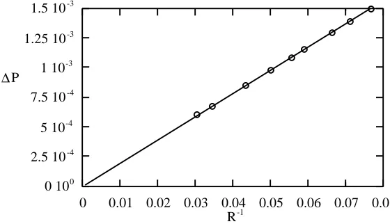
∆P R

= σ (10)

where ∆P is the change in pressure from the vapor to the fluid phase, σ is the surface tension, and R is the radius of curvature of the interface. As Swift et al1 demonstrate, the surface tension can be determined from the flat interface by

( )

σ=k

∫

2

(11)

Results of this test at a temperature T=0.55 with k=0.01, and ∆x =0.5 are shown in Fig. 1. The surface tension is calculated using Eq.(11) on a flat interface profile.

0 100 2.5 10-4 5 10-4 7.5 10-4 1 10-3 1.25 10-3 1.5 10-3

0 0.01 0.02 0.03 0.04 0.05 0.06 0.07 0.08 R-1

∆P

Fig. 1. Confirmation of Laplace’s Law. The solid line has a slope equal to the surface tension.

Figure 1 shows good correlation between the measured changes in pressure and those predicted by Laplace’s law. Other results, not shown here, for tests such as capillary wave simulation and coexistence curves of flat interfaces confirm Swift’s results as well.

Several difficulties with satisfying Galilean invariance in two-phase flows indicated in later literature9, motivate us to formulate additional benchmark test for validating the accuracy of LBM. First we need to elaborate on the Chapman-Enskog procedure, which is a method for solving the Boltzman evolution equation via asymptotic analysis. Again Mathematica is used to aid in the analysis. The procedure starts by performing an asymptotic expansion of a Taylor series expansion of the Boltzmann evolution equation. Specifically, a particle distribution expansion and a multi-scale time expansion are performed in terms of a Knudsen parameter δ defined as

δ = ∆tU

L (12)

and

f_σi f_σi δf_σ δ f_σ 0

i 1

i 2

= + + 2 +

.. .. ... (13)

∂t =∂t₀+δ∂t₁ +δ ∂t₂+ 2

... (14)

where ∆t is the time step, U and L are the characteristic velocity and length respectively, and

macroscopic evolution equations can be achieved. Further details of this procedure as applied to the square lattice are described by Hou et al8.

Final results of a Chapman-Enskog analysis for mass conservation are

∂ ρ ∂ ρt + _γ( u_γ)=O(δ2) (15)

and intermediate results for the conservation of momentum are

(

)

(

)

∂ ρt( u_α)+∂_β ∏_αβ − t_τ− _ ∂t ∏_αβ +∂_{γ γ} 



 

0 1 0

2 0

∆ f e_{σ σ}0_{i i} e_{σ α σ βi} e _i = O(δ2) (16)

with

αβ0

∏ = f e0_{i i} e _i

i

σ σ α σ β σ,

∑

If the fourth moment of the equilibrium distribution is evaluated, a substitution in Eq.(16) can be made

(

)

(

)

∂_γ f e_{σ σ}0_{i iγ}e_{σ α σ βi} e _i = c ∂ ρ_{β α} +∂ ρ_{α β} +∂ ρ_{γ γ} δ_αβ

2

3 ( u ) ( u ) ( u ) (18)

Rewriting Eq.(15) now yields

(

)

(

)

∂ ρt u_α ∂ ρ_β u u_{α β} ∂_{β αβ}P τ ∂ ∂ ρ_{β β α} ∂ ρ_{α β} ∂ ρ_{γ γ} δ_αβ

x t ( )+ ( )= − +(∆ ) ( − ) ( )+ ( )+ ( ) ∆ 2 2 1

6 u u u (19)

(

)

+∆t_τ−1_∂ ∂_{β t} ∏_αβ

2 0

0 _{+ O(δ}2₎

Further simplifications can be made to the momentum equation in two ways. The first is the introduction of a kinematic shear viscosity term υas

υ= (∆ ) ( τ− ) ∆ x t 2 2 1 6 (20)

The second simplification is an expression for ∂t₀∏_αβ0 as

(

)

∂t₀∏_αβ0 =∂t₀P_αβ+∂ ρt₀ u u_{α β}

(

)

[

]

[

]

= − ∂_{ρ αβ}P ∂ ρ_γ( u_γ) − u_{α γ βγ}∂ P +u_{β γ αγ}∂ P +∂ ρ_γ( u u u_{α β γ}) (21) If it is assumed that the kinematic bulk viscosity is equal to the kinematic shear viscosity, then the momentum equation takes on the form of

(

)

(

)

∂ ρt( u_α)+∂ ρ_β( u u_{α β})= −∂_{β αβ}P +υ ∂ ρ ∂_{β β}(u_α)+∂_α(u_β)+∂_γ(u_γ)δ_αβ (22)

(

)

(

)

+υ ∂_β u_{α β}∂ ρ( )+u_{β α}∂ ρ( )+u_{γ γ}∂ ρ δ( ) _αβ

(

)

−3 _{+ +}

2ν ∂β α γ βγ∂ β γ αγ∂ ∂ ργ α β γ

c u P u P ( u u u )

(

)

(

)

−3 ₊

2ν ∂ ∂β ρ αβ ∂ ργ γ

c P ( u ) O(δ

2₎

The top line of the momentum equation is the classical Navier-Stokes equation. All other terms are the error of LB model.

flows, and the error terms can not be ignored. In particular, the terms on the second line of Eq.(22) are of the same order as the shear force and momentum advection terms of the Navier-Stokes equation. These error terms are a source of non-Galilean invariance for the model.

Having identified the formal error terms in the momentum equation, the task arises for eliminating these terms or simply reducing them to the potential asymptotic accuracy of the model. The first step of this task is to evaluate the relative magnitudes of each of the error terms. From the static simulations near the critical point, it is known that the pressure variations from one phase to the next is generally small in comparison to the momentum of simple flows. Specifically, assume the gradient of pressure to be at most of order (u). Additionally, if ν is of order one, then the error of the third and fourth lines of Eq.(22) are at most of order of the Mach number squared. Upon this basis, the terms that remain to be considered are those on the second line of Eq.(22). One final comment about these dominant errors is that they result from defining the second equilibrium moment as the momentum and consequently are endemic to other models using this definition. A method for accounting for these errors is revealed if Eq.(22) is recast as

(

)

(

)

∂ ρt( u_α)+∂_β(∏_αβ )=υ ∂ ρ ∂_{β β α})+∂_α( _β)+∂_γ( _γ)δ_αβ

0

(u u u (23)

+υ ∂

(

(

)

)

This form of the momentum equation shows that to correct for the error terms on the second line, the equilibrium stress tensor should be modified

(

)

αβ0+ υ α β∂ ρ β α∂ ρ γ γ∂ ρ δαβ

∏ = P_αβ + ρu u_{α β}+ u ( )+u ( )+u ( ) (24)

By choosing this form for the equilibrium momentum tensor, the leading error terms of the momentum equation are eliminated at the small cost of introducing new lower order error terms. Applying the Chapman-Enskog procedure again produces the following momentum equation

(

)

(

)

∂ ρt( u_α)+∂ ρ_β( u u_{α β})= −∂_{β αβ}P +υ ∂ ρ ∂_{β β}(u_α)+∂_α(u_β)+∂_γ(u_γ)δ_αβ (25)

(

)

−3 _{+ +}

2ν ∂β α γ βγ∂ β γ αγ∂ ∂ ργ α β γ

c u P u P ( u u u )

(

)

(

)

−3

2ν ∂ ∂β ρ αβ ∂ ργ γ

c P ( u )

(

)

(

)

−3 2 _{+ +}

2

ν ∂_{β α γ}∂ _{β γ}∂ ρ _{γ β}∂ ρ _{λ λ}∂ ρ δ_βλ

c u u ( ) u ( ) u ( )

(

)

(

)

−3 2 _{+ +}

2

ν ∂_{β β γ}∂ _{α γ}∂ ρ _{γ α}∂ ρ _{λ λ}∂ ρ δ_αλ

c u u ( ) u ( ) u ( )

(

)

(

)

+3 2 _{+ +}

2 0

ν ∂ ∂_{β α β}∂ ρ _{β α}∂ ρ _{γ γ}∂ ρ δ_αβ

c t u ( ) u ( ) u ( ) +O(δ

2₎

The new momentum error terms are found in the last three lines of Eq.(25). Now, each of the error terms can be shown to be at most of order of the Mach number squared. Owing to the lower formal error of the new momentum tensor, this modified model is used for comparison with the original model in the following sections.

3. Results

those obtained using the original momentum tensor. Each simulation is performed with the parameters k=0.01, a=9/49, b=2/21, ∆x =0.5, ∆t =0.3, and τ =1 at a temperature T=0.55. Walls are modeled to meet the definitions of local density Eq.(1) and velocity Eq.(2) with the velocity perpendicular to the wall being zero5. With the choice of τ =1, the single particle distribution after the collision process equals the equilibrium distribution. Therefore, conditions at the wall are fully constrained. Finally, it is useful to introduce the dimensionless values

x x

L

+ _{= (26)}

y y

L

+ _{= (27)}

where L is the flow field size.

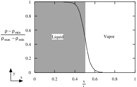
The first flow examined is Couette flow with the flow direction and fluid-vapor interface parallel to the y-axis in Fig. 2. A domain size nx=41 and ny=6 is used. The density profile is as shown in Fig. 2. This profile is consistent with static results in each of the simulations.

0 0.2 0.4 0.6 0.8 1

0 0.2 0.4 0.6 0.8 1

Liquid Vapor

y x

x L ρ ρ

ρ ρ

− −

min

max min

Fig. 2. Dimensionless density profile Couette flow simulation obtained by LBM. Key values are

ρmin=4.895 and ρmax=2.210.

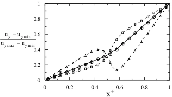
Two cases of Couette flow are run with this set-up . Case A is with the left plate fixed and right plate moving at a velocity (uy/c)(x+=1)=0.4, and case B with the right plate fixed and the left plate

moving with a velocity (uy/c)(x +

=0)=-0.4. Velocity results are found in Fig. 3. The exact velocity profile for this flow, assuming a Newtonian fluid, satisfies

τshear = constant =υρ∂xuy (28)

0 0.2 0.4 0.6 0.8 1

0 0.2 0.4 0.6 0.8 1

u u

u u

y y

y y

− −

mi n

max m in

x

Fig 3. Couette flow velocity profiles for case A original model(-- --), case A modified model( + ), case B original model(--∆--), and case B modified model( o ). The solid line is the finite difference solution.

Both case A and case B velocity profiles for the original model show highly non-physical trends in the interface. Also, these trends differ between the two cases: the slope of the velocity profile reverses sign at the interface. The presence and nature of this non-physical fluctuations is attributed to the dominant momentum error term

ν∂x(uy∂ ρx( ))≈O(1) (29)

The modified LB model takes into account this term and therefore yields velocity profiles for case A and B that are not only in agreement with the finite difference solution but also in agreement with each other. Since these velocity profiles are independent of the velocity of the reference frame, the modified model is Galilean invariant.

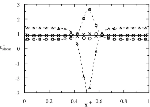
Shear stress profiles indicate how accurately the two LB models simulate Newtonian fluids. Figure 4 is a plot of the local non-dimensional shear stress

(

)

τ τ

ν ρ ρ

shear

shear

y y

L

u u

+ ₌ ⋅

+ 

 min max max− min

-3 -2 -1 0 1 2 3

0 0.2 0.4 0.6 0.8 1

τs hear+

x

Fig 4. Couette flow shear stress profiles for case A original model(-- --), case A modified model( + ), case B original model(--∆--), and case B modified model( o ). The solid line is the finite difference solution.

As mentioned previously, the shear stress should remain constant throughout the flow field. Although the modified model predictions do not match the exact profile (obtained via finite-difference approximation) in the interface region, the shear stress errors in this region are notably less error than those of the original model. More importantly however, the shear stresses in the bulk fluid regions obtained by the modified model match that predicted by the finite difference method in both cases A and B, whereas those obtained by the original model show considerable disagreement. This error of the shear stresses in the bulk fluid regions also play a large role in the shearing and advection of a droplet, as will be seen below.

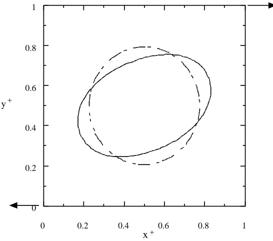
The second of the three flows examined is pure shear of a droplet. For this simulation, a developed droplet is placed between two plates which accelerate to the velocities (ux/c)(y+=1)=0.06 and (ux/c)(y+=0)=-0.06 as shown in Fig.(5). Simulations are performed on a grid

0 0.2 0.4 0.6 0.8 1

0 0.2 0.4 0.6 0.8 1

x+

y+

Fig. 5 . Single density contours for the partial shearing of a drop. The solid line is the result for the modified model developed here, and the dashed line for the original model.

This figure indicates that the droplet undergoes a larger shape deformation with the modified model than with the original model. Variations as this can be expected based on the Couette flow case A, where the shear stress for the original model was lower throughout the bulk regions of the fluid.

The final simulation reported here is that of the advection (translation) of a droplet. The setup is identical to the above with the exception that both the top and bottom plates are moved with a constant velocity (ux/c)= 0.06. For this simulation, it is useful to introduce the following

non-dimensional values

t tu

L

xwall

+_{= (31)}

u u

u

x x

xwall

+ _{= (32)}

-0.2 0 0.2 0.4 0.6 0.8 1

0 2 4 6 8 10

u

t

Fig.6. Droplet centroid velocity versus time where original model displacement rate is short dashes, original model local fluid velocity is medium dashes, modified model displacement is mixed dashes, and modified model local fluid velocity is the solid line.

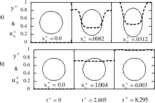
The original model results of Fig. 6. show a large scale divergence in the centroid velocity depending on how it is evaluated, and consequently both sets do not approach the velocity of the plates. Results for the modified model on the other hand are in close agreement and approach the velocity of the plates. For further insight into what is physically happening in this simulation, constant densities contours and centerline (y+=0.5) velocities are provided at three different times in Figs. 7a and 7b.

0 0.2 0.4 0.6 0.8 1

& a)

u_x+ y+

x_c+ =0 0. x_c+ =.0082 x_c+ =.0312

0 0.2 0.4 0.6 0.8 1

& b)

t+ =0 t+ =2 605. t+ =8 295.

u

y+

x_c+ =0 0. x_c+ =1 004. x_c+ =6 003.

Fig. 7 Density contours and centerline velocities for the original model(a) and modified model(b), where solid lines indicate a density of 3.5, dashed lines indicate center line velocity ux(y+=0.5),

and xc is the location of the center of the drop at time t.

on the Chapman-Enskog procedure results. The original model is conserving mass and momentum locally, yet it does not satisfy the Navier-Stokes equation. The system satisfies conservation of mass by allowing high velocities in the vapor region and low velocities in the liquid region. However, since conservation of momentum is not satisfied, the drop does not advect correctly, but rather forms a “standing wave” of mass. In contrast, results for the modified model indicate the drop maintains its shape, the velocities throughout the flow field approach the velocity of the plates, and are fairly constant in the fully developed stage.

4. Conclusions

Based on the results of the benchmark flows and discussion presented, three main conclusions can be drawn. First, the two-phase flow LB model introduced by Swift et al1 exhibits non-physical aberrations (manifested by lack of Galilean invariance) owing to the truncation of non-negligible terms in the momentum equation expansion. This has been addressed in a preliminary fashion by Osborn et al9. Second, it is possible to incorporate these terms in the formal expansion by re-defining the stress tensor and thus recover Galilean invariance. Our results with the three benchmark flows demonstrate that the modified LB model closely approximates the Navier-Stokes equations in regions of high density gradients (typical of two-phase flow). Similarly, this correction method could be applied to reduce other sources of error as in flow domains exhibiting large pressure gradients.

Acknowledgments

1 _{M. Swift, W. R. Osborn, and J. M. Yeomans, Phys. Rev. Lett. 75, 830 (1995)} 2 _{S. Chen and G. D. Doolen, Ann. Rev. Fluid. Mech. 30, 329(1998)}

3 _{X. Shan and H. Chen, Phys. Rev. E 47, 1815 (1993)}

4 _{X. He, X. Shan, and G. D. Doolen, Phys. Rev. E 57, R13 (1998)} 5

V.P. Carey and N.E. Hawks, ASME J. Heat Trans. 117, 432 (1995)

6 _{D. Noble, S. Chen, J. G. Georgiadis and R. Buckius, Phys. Fluids 7, 203 (1995)} 7 _{D. Jasnow and J. Vinals, Phys. Fluids 8, 660 (1996)}

8 _{S. Hou, Q. Zou, S. Chen, G. Doolen, and A. C. Cogley, J. Comp. Phys. 118, 329 (1995)} 9