A Comparison of Classical and Bayesian GARCH Models
Farhat Iqbal
Department of Statistics, University of Balochistan Quetta-Pakistan
Abstract
This paper is concerned with the estimation, forecasting and evaluation of Value-at-Risk (VaR) of Karachi Stock Exchange before and after the global financial crisis of 2008 using Bayesian method. The generalized autoregressive conditional heteroscedastic (GARCH) models under the assumption of normal and heavy-tailed errors are used to forecast one-day-ahead risk estimates. Various measures and backtesting methods are employed to evaluate VaR forecasts. The observed number of VaR violations using Bayesian method is found close to the expected number of violations. The losses are also found smaller than the competing Maximum Likelihood method. The results showed that the Bayesian method produce accurate and reliable VaR forecasts and can be preferred over other methods.
Keywords: GARCH, Volatility, Value-at-Risk, MCMC.
1. Introduction
Value-at-Risk (VaR) has become a popular tool and is widely used for risk management and capital allocation by financial institutions. Both underestimation and overestimation of risk could have a negative effect in financial markets. Therefore accurate estimates of VaR is crucial for the financial stability of markets. VaR can be defined as the quantile of the loss, during a specific time period, that can occur within a given portfolio. A precise quantile estimate far out in the left tail of the return distribution is desirable. A thorough survey of risk measures is provided by Jorion (2007).
Various approaches for estimating and predicting VaR exist in literature. These include nonparametric method such as historical simulation; semi-parametric method based on extreme value theory and quantile regression method and full parametric models (see McNeil and Frey, 2000 and Engle and Manganelli, 2004, among others). Kuester et al. (2006) provided an overview and comparisons of these and further methods whereas a comprehensive overview is found in Abad et al. (2014).
Under the parametric statistical approaches, the autoregressive conditional heteroscedastic (ARCH) model of Engle (1982) and generalized ARCH (GARCH) model of Bollerslev (1986) are widely-used by researchers and practitioners. These models can capture the conditional variance structure and some of the stylized facts of many financial time series. Since then numerous extensions of the GARCH model have been proposed. Among them, the exponential GARCH model of Nelson (1991) and asymmetric model of Glosten et al. (1993) are popular. Accurate volatility estimates are essential for producing reliable VaR estimates.
estimator (QMLE). However, normality is often rejected in applications as the unconditional distribution of most financial asset returns has fatter tails than implied by this model with normal errors. The excess of (unconditional) kurtosis has been most commonly accommodated with Student-t distributed errors (e.g. Baillie and Bollerslev, 1989). Besides, robust methods for the estimation of GARCH models are also suggested (Peng and Yao, 2003; Muller and Yohai, 2008; Iqbal and Mukherjee, 2010 to cite few)
Another approach to estimate the parameters and volatility of GARCH model is to use Bayesian framework. The Bayesian paradigm offers a natural way of taking both parameter uncertainty and model uncertainty into account. However, the literature on Bayesian treatment of GARCH model in not as enormous as in the case of QMLE. In Bayesian setup, most of the time a researcher has to rely on computational methods such as Markov Chain Monte Carlo (MCMC) for the estimation of these models (see Nakatsuma, 1998, 2000, Ardia, 2008 and Deschamps, 2012).
Karachi Stock Exchange (KSE) is the major stock market of Pakistan. Most of the studies on risk estimated of KSE that exist in literature applied classical methods for estimation and prediction. Iqbal et al. (2010) used four different parametric methods and two non-parametric methods for VaR computation of KSE. Qayyum and Nawaz (2010) used extreme value theory and Nawaz and Afzal (2011) computed the VaR using Historical Simulation and Risk Metrics method. Mahmud and Mirza (2011) forecast the volatility of KSE before and after the financial crisis using GARCH models. Haque and Naeem (2014) investigated the volatility forecasting performance of GARCH models with various distribution of innovations. To the best of our knowledge, the Bayesian framework has not been yet applied for volatility or risk forecasting of KSE. This motivate us to fill this gap and contribute to the literature.
The main aim of this paper is to estimate and forecast VaR using GARCH models in Bayesian setup. The QMLE method is also used for the comparison of results. The estimates and forecasts of volatility and VaR are computed by these two methods using Gaussian and Student-t distributions for innovations. Various evaluation measures and backtesting methods are employed to compare the in-sample and out-of-sample forecasts of VaR. The daily closing prices of KSE from January 03, 2005 to December 30, 2011 are used in the present study. This study is important from various angles. First, as aforementioned, the VaR estimates of KSE are calculates using Bayesian method that to the best of our knowledge has not been studied. Another contribution of this study is to check the effects of large shocks on risk estimated of KSE not only in the full time period but also before and after the global financial crisis. This may help practitioners and researchers to understand the behaviour of risk measure when the market is hit by large shocks at different time periods and their after effects. Finally, the use of Bayesian method for forecasting in GARCH model may encourage academicians and researchers in Pakistan to apply Bayesian methods for local financial data.
2. GARCH Model and Estimation
For the simple GARCH (1, 1) model, the following representation of the return series
is assumed. Observer such that
(2.1)
,
where is a sequence of independent and identically distributed (i.i.d.) unobservable real-valued random variables with mean 0 and variance 1 and distribution D; and
[ ] the unknown parameter vector in the parameter space
[ ]
Under these parameter constratints, The GARCH(1,1) model in (2.1) is strictly stationary and hence covariance stationary under finite second moment.
In this study, two error distributions are used for the i.i.d innovations. The choice
is a standard and Student-t distribution. Th later is standardized to have zero mean and unit variance.
The conditional likelihood can be written as:
∏
√ (√ )
where and is the relevant error density function of . In the classical setup, is assumed to be the true and fixed value and the maximum likelihood estimator of is then obtained by
̂
In the Bayesian setup, is considered to be a random variable with a prior density which depends on the researcher’s prior belief. These parameters are assumed to be a priori independent and normally distributed truncated to the intervals that define each one. It is also assumed that few known and constant hyperparameters specify their densities. For example, as proposed in Ardia (2008), these are given by
and ( ) , where is the indicator function.
The posterior density of is obtained using the Bayes’ rule as
∫
Metropolis-Hasting algorithm (Metropolis et al., 1953 and Hasting, 1970) and the Gibbs sampler (Geman and Geman, 1984), among others.
For the GARCH (1,1) model in (2.1) and assuming , the likelihood function of can be written as:
[ ]
where and is the determinant of a matrix. The likelihood for Student-t distribution can also be written in a similar fashion with additional parameter, , the degress of freedom, that is also estimated with the parameters. For a comprehensive details of MCMC method in GARCH model, interested reader are referred to Nakatsuma (1998) and Ardia (2008).
3. Value-at-Risk Forecasting and Evaluation
This section first describes the method of predicting VaR using GARCH model. Then, evaluation measures and bactesting methods are presented to evaluate these VaR estimates. VaR measures the worst expected loss of a portfolio over a target horizon at a given confidence level, due to an adverse movement in the relevant security price (Jorion, 2007). For a known probability , a VaR is defined as the thconditional quantile of the returns. Hence the VaR at time for the returns is defined as
where is the conditional distribution of given then information available up to . Hence, from (2.1) we get where is the quantile function of the innovation . The estimate of VaR is then defined as
̂ ̂ ( ̂ ) [ ] { ̂ ⁄ ̂ } (3.1)
The Basel Committee on Banking Supervision (1996) recommends a backtesting procedure to evaluate the accuracy of VaR forecasts. This is generally based on the number of observed violations, i.e. when actual losses exceed VaR in a sample period.
3.1 Coverage probability and violation rate
Let us define the total number of observed violations as
∑
̂
Then the closeness of empirical rejection probability ̂ to ‘ ’ can be used to assess the overall predicative performance of the VaR model. This probability also known as VaR violation rate provides an interesting insight to VaR forecasts.
models. Of course, a model with this ratio close to unity is prefered and in case of ties, conservative model ( ̂ ) is chosen as superior .
3.2 Average quadratic loss
The magnitude of losses is also important in the evaluation of VaR. Lopez (1999) considered this magnitude and defined the average quadratic loss (AQL) of a VaR estimate. The overall AQL of a VaR estimate is obtained as ∑ where
{ ̂ ̂ ̂
Next, we define formal tests for backtesting VaR estimates.
3.3 Coverage tests
The first test is the unconditional likelihood ratio test proposed by Kupiec (1995). It is defined as
[ ̂ ̂ ]
which is asymptotically .
Christoffersen (1998) defined the independence coverage test statistic, denoted by as follows. For let denotes the number of time points for which is followed by . Let
̂ ⁄ ̂ ⁄
Then
[ ( ̂ ̂
̂ ̂ ) ( ̂ ̂ )]
The conditional coverage test statistic of Christoferssen (1998) which is asymptotically
is
3.44 Dynamic quantile test
Higher order dependence in VaR violations also need to be checked. The dynamic quantile (DQ) test of Engle and Manganelli (2004) is used for this purpose. This test is described as follows. Let the th response be
{ ̂ ̂
and . Consider a linear regression model with response [ ] and a
design matrix [ ] with and all ones in the first column. For the
th term with if and if and ̂ . The DQ test statistic is asymptotically and is defined as
̂ ̂
These measures and tests are used in this study to evaluate and compare the performance of risk estimates of QMLE and Bayesian method.
4. Empirical Results and Discussion
4.1 Data and preliminary analysis
The present study uses the daily closing prices of Karachi Stock Exchange (KSE 100 Index). The dataset is obtained from the http://finance.yahoo.com for the period of January 03, 2005 to December 31, 2011. This period include the high volatile period because of the global financial crisis. This may help us to understand the dynamics of KSE before and after the financial crisis. The full data set consists of 1686 observations. The data is later divided into two periods: the pre-crisis period (03 January 2005 – 30 August 2008) consisting of 907 observations, and the post-crisis period (01 September 2008 – 31 December 2011) having 779 data points. The KSE was almost static for few weeks during the last quarter of 2008 and therefore few observations (from 09 October 2008 – 12 December 2008) are removed.
The returns at time is defined as , where is the closing index of KSE at time . Then using ̅ (with
̅ ∑ ) as our observations, the whole span in each time period is divided into two parts: the estimation or in-sample part of initial observations used for estimating the unknown parameters in GARCH models and the validation or out-of-sample part of
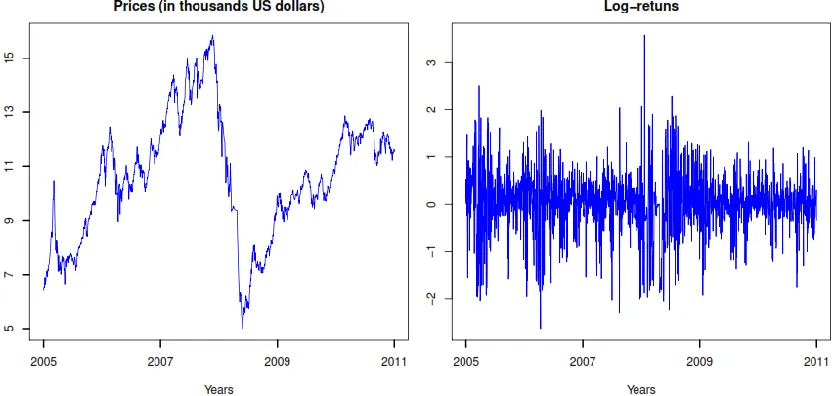
observations for the prediction and assessment of VaR. For out-of-sample forecasting, which corresponds to one year observations. The recommended back-testing guideline proposed by the Basel Committee on Banking Supervision (1996) is to also evaluate a one percent (1%) VaR model over a 12 month test period (250 trading days). The daily closing prices (in thousands US dollar) and log-returns of KSE are shown in Figure 1 below. The effect of global financial crisis is evident on KSE. A large drop in the prices and high volatility and volatility clustering can also be seen in in log-returns.
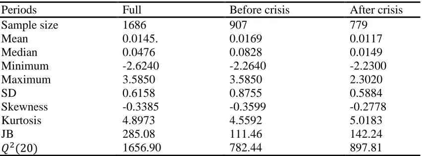
Table 1 presents the summary statistics for the full, before the crisis and after the crisis time periods. These statistics may help us to examine the behaviour of the stock returns. All time periods have higher kurtosis and negative skewness in returns. The normality in returns was tested using Jarque-Bera test for normality and high values of this test show that the KSE returns are significantly different from normality. High values of Ljung-Box ( ) statistic for the squared returns at lag 20 were also observed in all time periods. This is the indication of dependence in squared returns and thus a need for fitting GARCH models. In summary, the KSE return series do not conform to normal distribution, display negative skewness (the distribution has a long left tail) and high kurtosis (fat tails) for all periods. It can also be noticed that the unconditional volatility is higher just before the crisis period.
Table 1: Summary statistics for daily return of Karachi Stock Exchange
Periods Full Before crisis After crisis
Sample size 1686 907 779
Mean 0.0145. 0.0169 0.0117
Median 0.0476 0.0828 0.0149
Minimum -2.6240 -2.2640 -2.2300
Maximum 3.5850 3.5850 2.3020
SD 0.6158 0.8755 0.5884
Skewness -0.3385 -0.3599 -0.2778
Kurtosis 4.8973 4.5592 5.0183
JB 285.08 111.46 142.24
1656.90 782.44 897.81
Note: Full period (03 January 2005 – 31 December 2011); Before crisis period (03 January 2005 – 30 August 2008); After crisis period (01 September 2008 – 31 December 2011); JB (Jarque-Bera statistic for normality of return); (Ljung-Box statistics at lag 20 for serial correlation in squared returns).
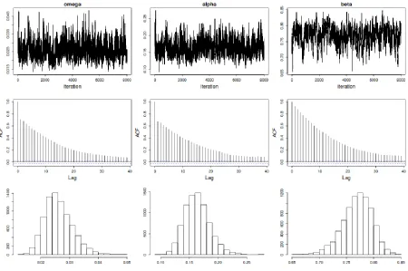
Next, the GARCH model is fitted to all three time periods. The in-sample estimates of parameters, volatility and VaR are obtained using the QMLE and Bayesian method under the assumptions of both Gaussian and Student-t distributions. For the MCMC method, a total of 10,000 iterations are run discarding the first 2,000 realizations as burn-in period. Posterior results are then based on 8,000 realizations of the Markov chain with the prior distributions as explained in Section 2. The simulated Markov chains are checked for convergence and good mixing by visual inspection of the marginal traces, density estimates, and autocorrelations are observed. Figure 2 shows an illustration of the diagnostic plots.
4.1 In-sample VaR analysis
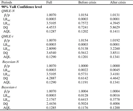
methods produce reasobaly indentical results for the full time period. The observed ratios ̂ were found close to 1 which means that the number of observed violations are close to expected number of violations. The results of all three tests (unconditional and conditional coverage tests and dynamic quantile test) values divided by their respective critical values at 5% confidence level are also reported. A value greater than 1 means rejection of the test at 5% level. Non-significant values for unconditional coverage test and significant values for conditional coverage and DQ test are found using QMLE. In Bayesian method, again only unconditional test is found non-significant. The average quadratic loss (AQL) produced by both methods are similar in magnitude.
For other two time periods (before and after financial crisis) considered in this study, some interesting findings are noticed. The expected and observed number of violation in Bayesian showed exactly same values, therefore VaR ratios of 1 can be seen in these periods. The number of observed violation for QMLE are found smaller than the expected violations. In after crisis period the conditional coverage and DQ tests are also rejected by QMLE whereas non-significant values of these test statistics in Bayesian confirms independence of violations from their lags and past VaR. Finally, the AQL of Bayesian is also found smaller than the QMLE in both time periods meaning that the losses using Bayesian are less on average.
The result of in-sample VaR when Student-t distribution was assumed for errors showed similar trend. With Bayesian method outperforming the QMLE in terms of better VaR ratios, nonsignificant test statistics and lower AQL. Another feature that can be observed is that these results get slightly better than those in Gaussian case. This indicates that Student-t distribution is preferred for better risk forecasting in GARCH models. In summary, the Bayesian method provides reliable VaR forecasts than the QMLE and further improves the forecasts when heavy-tailed distribution is assumed for errors.
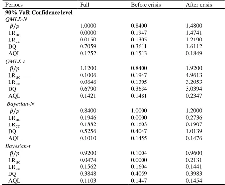
4.2 Out-sample VaR analysis
For policy and risk management, prediction and evaluation of VaR are considered more important. This subsection highlights the results of out-of-sample VaR forecats. To produce one-day-ahead forecast of VaR, a rolling window approach is used. More specifically, the model is fitted to the estimation period using in-sample part of K observations and one-day-ahead forecasts are obtained. Then the in-sample period is rolled forward by one day dropping the first observation. The model is re-estimated and again the next day forecasts are obtained. In this way out-of-sample VaR forecasts of approximately one year (250 days) are obtained for the forecast period using both methods.
Table 2: In-sample VaR evaluation using GARCH model
Periods Full Before crisis After crisis
90% VaR Confidence level
QMLE-N
̂ 1.0070 1.0154 1.0131
0.0003 0.0003 0.0001
3.5105 0.7572 4.3945
4.4533 0.7241 5.8629
AQL 0.1287 0.1202 0.1411
QMLE-t
̂ 1.0070 1.0154 1.0192
0.0003 0.0003 0.0001
2.8090 0.5138 3.2260
3.6540 0.5612 3.8511
AQL 0.1290 0.1201 0.1341
Bayesian-N
̂ 1.0070 1.0000 1.0000
0.0003 0.0022 0.0045
3.5105 0.5731 3.4181
4.2887 0.6142 4.4642
AQL 0.1290 0.1191 0.1341
Bayesian-t
̂ 1.0070 1.0004 1.0004
0.0003 0.0128 0.0016
2.1767 0.6415 0.3778
2.4436 0.5024 0.4006
AQL 0.1285 0.1176 0.1200
Note: Full period (03 January 2005 – 31 December 2011); Before crisis period (03 January 2005 – 30 August 2007); After crisis period (01 September 2008 – 31 December 2013); (Dynamic quantile statistic); AQL (Average quadratic loss); the smallest AQL is in bold type; For all three tests, >1 means rejection at 5% level.
5. Conclusion
This study can be extended in following ways: The MCMC method used is very time consuming. New and efficient Bayesian methods such as Sequential Monte Carlo can be used for online estimation and prediction of GARCH models. A simple GARCH model is studied whereas other variants that consider asymmetry and jumps in volatility can be considered and may provide better risk forecasts.
Table 3: Out-of-sample VaR evaluation using GARCH model
Periods Full Before crisis After crisis
90% VaR Confidence level
QMLE-N
̂ 1.0000 0.8400 1.4800
0.0000 0.1947 1.4741
0.0150 0.1305 1.2190
0.7059 0.3611 1.6112
AQL 0.1252 0.1513 0.1849
QMLE-t
̂ 1.1200 0.8400 1.9200
0.1006 0.1947 4.9613
0.0646 0.1305 3.2053
0.6790 0.3634 3.0394
AQL 0.1421 0.1481 0.2347
Bayesian-N
̂ 0.8400 1.0000 1.2000
0.1946 0.0000 0.2736
0.1882 0.1603 0.1907
0.5256 0.4047 1.0139
AQL 0.1010 0.1455 0.1476
Bayesian-t
̂ 0.9200 0.1004 0.9600
0.0474 0.0000 0.2131
0.1562 0.1604 0.1441
0.3848 0.4059 0.3983
AQL 0.1103 0.1447 0.1454
Note: Full period (03 January 2005 – 31 December 2011); Before crisis period (03 January 2005 – 30 August 2007); After crisis period (01 September 2008 – 31 December 2013); (Dynamic quantile statistic); AQL (Average quadratic loss); the smallest AQL is in bold type; For all three tests, >1 means rejection at 5% level.
References
1. Abad, P., Benito, S. and Lopez, C. (2014). A comprehensive review of Value at Risk methodologies. The Spanish Review of Financial Economics. 12: 15 – 32.
2. Ardia., D. (2008). Financial Risk Management with Bayesian Estimation of
3. Baillie, R. and Bollerslev, T. (1989). The message in daily exchange rates: A conditional-variance tale. Journal of Business and Economic Statistics. 7(3): 297– 305.
4. Basel Committee on Banking Supervision. (1996). Supervisory framework for the use of Backtesting in conjunction with the international model-based approach to market risk capital requirements. BIS, Basel, Switzerland.
5. Bollerslev, T. (1986). Generalised autoregressive conditional heteroscedasticity.
Journal of Econometrics. 31(3): 307 – 327.
6. Christoffersen, P. (1998). Evaluating interval forecasts. International Economics
Review. 39: 841–862.
7. Deschamps, J.P. (2012). Bayesian estimation of generalized hyperbolic skewed student GARCH models. Computational Statistics & Data Analysis. 56(11): 3035–3054.
8. Engle, R.F. (1982). Autoregressive Conditional Heteroskedasticity With Estimates of the Variance of U.K. Inflation. Econometrica. 50: 987 – 1008.
9. Engle, R.F. and Manganelli, S. (2004) CAViaR: conditional autoregressive value at risk by regression quantiles. Journal of Business and Economic Statistics. 22: 367–381.
10. Geman, S. and Geman, D. (1984). Stochastic relaxation, Gibbs distributions, and the Bayesian restoration of images. IEEE Transactions on Pattern Analysis and
Machine Intelligence. 6: 721 – 741.
11. Glosten, L. Jagannathan, R. and Runkle, D. (1993). On the relation between the expected value and the volatility on the nominal excess return on stocks. Journal
of Finance. 48(5): 1779 – 1801.
12. Hastings, W. (1970). Monte Carlo sampling methods using Markov chains and their applications. Biometrika. 57: 97–109.
13. Haque, A. and Naeem, K. (2014). Forecasting volatility and Value-at-Risk of Karachi Stock Exchange 100 Index: Comparing distribution-type and symmetry-type models. European Online Journal of Natural and Social Sciences. 3(2): 208– 219.
14. Iqbal, J., Azher, S. and Ijaz, A. (2010). Predictive ability of Value-at-Risk methods: evidence from the Karachi Stock Exchange-100 Index. MPRA Paper 01/2010, University Library of Munich, Germany.
15. Iqbal, F. and Mukherjee, K. (2010). M-estimators of some GARCH-type models; computation and application. Statistics and Computing. 20: 435 – 445.
16. Jorion, P. (2007). Value at Risk: The New Benchmark for Managing Financial Risk. 3rd edn, McGraw-Hill, New York.
18. Kupiec, P.H. (1995) Techniques for verifying the accuracy of risk measurement models. Journal of Derivatives. 3: 73–84.
19. Lopez, J.A. (1999). Methods for evaluating value-at-risk estimates. Economic
Review. 2: 3–17.
20. Mahmud, M. and Nawazish, M. (2011). Volatility and dynamics in an emerging economy: Case of Karachi Stock Exchange. Ekonomska Istraživanja. 24(4): 51–64.
21. Metropolis, N., Rosenbluth, A., Rosenbluth, M., Teller, A. and Teller, E. (1953). Equations of state calculations by fast computing machines. Journal of Chemical
Physics. 21: 1087–1091.
22. McNeil, A.J. and Frey, R. (2000). Estimation of tail-related risk measures for heteroscedastic financial time series: an extreme value approach. Journal of
Empirical Finance. 7: 271–300.
23. Muller, N. and Yohai, V.J. (2008). Robust estimates for GARCH models. Journal
of Statistical Planning and Inference. 138: 2918 – 2940.
24. Nakatsuma, T. (1998). Markov-Chain Sampling Algorithm for GARCH Models. Studies in Nonlinear Dynamics and Econometrics. 3(2): 107 – 117.
25. Nakatsuma, T. (2000). Bayesian Analysis of ARMA-GARCH Models: A Markov Chain Sampling Approach. Journal of Econometrics. 95(1): 57 – 69.
26. Nelson, D.B. (1991). Conditional Heteroskedasticity in Asset Returns: A New Approach. Econometrica. 59: 347 – 370.
27. Nawaz, F. and Afzal, M. (2011). Value at risk: Evidence from Pakistan Stock Exchange. African Journal of Business Management. 5(17): 7474–7480.
28. Peng L. and Yao Q. (2003). Least absolute deviations estimation for ARCH and GARCH models. Biometrika. 90: 967 – 975.