ARITHMETIC CONSTRUCTIONS OF BINARY SELF-DUAL CODES

ARITHMETIC CONSTRUCTIONS OF BINARY SELF-DUAL

CODES

Ying Zhang

A Dissertation

in

Mathematics

Presented to the Faculties of the University of Pennsylvania in Partial

Fulfillment of the Requirements for the Degree of Doctor of Philosophy

2013

Advisor’s Name

Supervisor of Dissertation

ABSTRACT

ARITHMETIC CONSTRUCTIONS OF BINARY SELF-DUAL CODES

Contents

1 Introduction 1

2 Coding Theory Backgrounds 4

2.1 General Codes . . . 4

2.2 Binary Self-dual Code . . . 7

2.2.1 Extremal Code . . . 10

3 Construction _Q 12 3.1 S-integers . . . 13

3.2 Hilbert Symbols . . . 13

3.3 The Construction . . . 16

3.4 A Random Generation Algorithm . . . 23

4 Construction G 27 4.1 Arithmetic Duality . . . 28

5 Equivariant Construction 37

5.1 Borel’s Equivariant Cohomology . . . 38

5.2 Equivariant Etale Sheaves . . . 40

5.3 The Localization Theorem . . . 44

5.4 Equivariant Construction . . . 49

5.5 Comparison with Construction G . . . 53

5.6 The Maximality Condition . . . 61

A Topological constructions of binary self-dual codes 68

B The Minimal Hirsch-Brown Model 73

Chapter 1

Introduction

The goal of this thesis is to explore the interplay between binary self-dual codes and ´etale cohomology of arithmetic schemes. In chapter 2, we will recall some definitions and general facts of codes. A construction of binary self-dual code is introduced in chapter 3 using arithmetics of the rational number field _Q (which we call Construction _Q). Construction _Q shows that up to equivalence, all binary self-dual codes have a simple description (not necessarily unique) using a boxed matrix, see table 3.1. Starting from chapter 4, the focus of the thesis will be mainly on arithmetic questions inspired by the search of binary self-dual codes. Two more constructions of binary codes are introduced and compared, which we call Construction G and Equivariant Construction.

M. Freedman showed that for each unimodular symmetric bilinear form over _Z, there is a simply-connected compact 4-manifold M whose intersection form

H2(M,_Z)×H2(M,_Z)→_Z

realizes this bilinear form [Fre82]. In fact, this bilinear form “almost determines” the homeomorphism type of the manifold M and puts restriction on when it has smooth structures [GS99].

For an involution τ on a closed manifold, it is well known the cohomology of the fixed loci is related to that of the manifold. In a series of recent papers by Puppe [Pup95], [Pup01], Kreck and Puppe [KP08], this relation is explored to construct binary self-dual codes when τ has isolated fixed points. For convenience of the reader, part of their work is reviewed in appendix A. In particular, we review two constructions of theirs: theTopological Equivariant Construction and Poincar´e Duality Construction. It is these constructions that inspired our constructions over

arithmetic schemes.

As a matter of fact, our Construction _Q and Construction G are analogues to the Poincar´e Duality Construction. The Equivariant Construction and Topological Equivariant Construction are developed in a common framework. This is not sur-prising since the classical motivation of ´etale cohomology is to seek “topological” treatment of schemes.

Chapter 2

Coding Theory Backgrounds

2.1

General Codes

In this section we will collect some terminologies in coding theory. The main purpose is to set up notations which will be used in later parts of the thesis. For a more complete introduction to the subject, the readers are referred to standard texts like [CS99, Chapter 3][PH][Ple98].

Let _F be a finite set called the alphabet. An element in the set _Fn _{is called a}

required to be a non-unital sub-ring. In this thesis we will only consider linear code over a field _F.

When C is a linear code in an n-dimensional space W/_F, we will assume W

is equipped with a chosen set of basis E under which we can write W = _Fn_{. In}

the existing literature in coding theory, an n-dimension vector space W is often explicitly given as _Fn_{, with an assumed basis which becomes the canonical basis in}

Fn. However, in our later constructions of codes from abstract cohomology space,

a “canonical” basis is usually not obvious in W. In some cases, the existence of a desirable basis is even in question, see ??.

Under the canonical basis in _Fn_{, consider a word u = (u}

1,· · · , un). The

Ham-ming weight ofuis the number of nonzero componentsui, denoted bywt(u). Given

a codeC, we can count the total number of words of each possible weight and store these counts in a vector, called the weight distribution vector of C.

For ann-dimensional _Fvector space W, h, i: W×W →_Fis a non-degenerate bilinear form if it satisfies the following conditions:

• hx+y, zi=hx, zi+hy, zi.

• hx, y+zi=hx, yi+hx, zi.

• if hx, yi= 0 for all y∈W then x= 0,

• if hx, yi= 0 for all x∈W then y= 0.

Suppose _F is equipped with an involution (which could be trivial), denoted by a bar, satisfying

x=x, x+y=x+y, xy=x y

We require

hx, yi=hy, xi,hax, yi=hx, ayi

Given a non-degenerate bilinear form h,i, for a code C ⊂ W, we can define its dual code

C⊥ :={x∈W|∀y∈C,hx, yi= 0}

IfC⊥ ⊆C,Cis calledself-orthogonal. WhenC⊥ =C,Cis called self-orthogonal of maximal dimension.

Example 2.1.1 (Main Example). Under a basis E in an n-dimensional space W/_F, define the product of two words x= (x1,· · · , xn), y= (y1,· · · , yn) by

hx, yi=

n

X

i=1 xiy¯i

This product satisfies the above requirements. For a bilinear form h,i, if there is a basis E under which the form is defined as above, then h,i is called an inner product. When the involution is trivial, we will call it a Euclidean inner product;

the basis E will be called aEuclidean basis. 4

In the main part of the thesis, we will only focus on the case when _F = _F2 =

2.2

Binary Self-dual Code

Consider anmdimension vector spaceW over_F2 with a basisE. We can define the

inner product associated to this basis. IfC is anndimensional self-orthogonal code of maximal dimension, then m = 2n is even. We will require thatE is specified as an ordered basis {ei}mi=1. The triple (W, E, V) is called a binary self-dual code of

length m.

For a code word over _F2, the Hamming weight of the word is just the number of ones in the word. A word that is self-orthogonal has even weight. In addition, if the Hamming weight of each word in a binary self-dual code C is a multiple of 4, we will say C is a Type II code, or adoubly even code. If not, C is called aType I code or a singly even code. IfW has a Type II code contained in it, the dimension of W is necessarily a multiple of 8 [RS98].

Two self-dual codes (W, V, E), (W0, V0, E0) are defined to be equivalent if there is a bijection between E and E0 which when extended to an _F2-linear isomorphism W → W0 maps V to V0. Alternatively, fixing W, if there is a permutation of the basis E that mapsV toV0, then the two codes (W, E, V) and (W, E0, V0) are called equivalent. The permutations on the ordered basisE that map the spaceV to itself will constitute the automorphism group of the code. Obviously, the automorphism group of a code is a subgroup of the symmetric group S2n. If V is equivalent toV0,

then their automorphism groups are conjugate to each other in S2n.

allx, y ∈W A is said to be an element in theorthogonal group O(m) associated to

h,i. Under a basis E, A can be represented by an element inGLm×m(F2).

Fixing E, a generator matrix is a matrix whose row vectors span a basis for a code. For example, a generator matrix for a binary self-dual code is ann×2nmatrix of rank n. Up to equivalence, every self-dual code has a generator matrix of the form [In, Pn] where Inis the n×n identity matrix, and Pn ∈O(n) is an orthogonal

matrix. Let O(2n) act on W by left multiplication. Since O(n) ,→ O(2n) in the lower right corner, the action of O(2n) is transitive on the set of self-orthogonal spaces V of maximal dimension. This explains why in the definition of equivalence relation we only consider a permutation rather than a general orthogonal change of basis: had we chosen the latter, the definition of equivalence class of codes would not be interesting.

Remark 2.2.1. A useful fact is that for the Euclidean form, O(n) coincides withSn

if and only if n≤ 3. Indeed, whenn ≤3 it is obvious. An example for an element in O(4)_rS4 is provided by the generator matrix for the length 8 binary self-dual

code e8. ♦

Denote by T2n the set of all distinct self-dual codes of length 2n. There is a

simple counting formula

|T2n|= Πni=1−1(2

i_{+ 1)}

When m is divisible by 8, the total number of Type II codes is

Denote the orbit of C under the S2n action by CE. |CE| =

|S2n|

|Aut(C)|. Thus we have:

|T2n|=

X Inequivalent C

|S2n|

|Aut(C)| (2.2.1)

We will define

pC :=

|CE|

|T2n|

(2.2.2)

as the density of the equivalence class CE inT2n.

The following result of [OP92] is relevant. Denote the set of codes that have a non-trivial automorphism group by A2n, then

Proposition 2.2.2 (Rigidity).

lim

n→∞

|A2n|

|T2n|

= 0

Therefore when n gets big, most codes have density dC =

(2n)!

|T2n|.

Remark 2.2.3. One should use caution in such a statement. Based on [OP92] along, it does not qualify to say “most equivalence classes” have the abovedC, since codes

with bigger automorphism groups could conceivably break up into more equivalence classes. The author have not seen this question being addressed in the literature. ♦

Equivalent to Equation 2.2.1, one can write

X InequivalentC

1

|Aut(C)| =

T2n

(2n)! (2.2.3)

Equation 2.2.3 is often called the mass formula in the literature. When k is any number smaller than 1₂, Tn

(2n)! grows faster than e

kn2

of classifying inequivalent codes of given length is computationally costly. For the reader’s interest, there are now several on-line databases of equivalence classes of binary self-dual codes. For example, A. Munemasa summarized on his website a complete list with length up to 40.

2.2.1

Extremal Code

Coding theory has interesting connections with other branches of mathematics, in-cluding combinatorial design, lattice theory and invariant theory [CS99, Chapter 3][PH][Ple98]. Codes are also used for error-correcting purposes in telecommuni-cation. Some of the best error-correction codes are binary self-dual codes. For error-correction purposes, the relevant combinatorial property is the weight distri-bution of the code. In particular, its non-zero minimal weight is important, which is an even integer. For a code C of length 2n, denote its minimal distance by d2n.

Two questions are of general interest:

Question 2.2.4. Fixing the length 2n, what is the largest minimal weight d2n?

Fixing length 2n, we will call a code with the largest minimal weight anextremal code. When 2n range between [56,110], not all the extremal codes (or in some cases even the d2n) are known [DGH97]. Other than the extremal codes, the existence

with smaller length; or a systematic study of “descendants” of codes of smaller length. See the references listed above together with [KB12][BB11]. Based on our Construction_Q, we propose a “probabilistic” method of generating binary self-dual code, 3.4.

Question 2.2.5. What is lim sup _m→∞ dm

m?

For this question we quote the following result for a lower bound:

Proposition 2.2.6. [RS98, section 10] There is an infinite sequence of codes Ci

where the ratio di

Chapter 3

Construction

_Q

In this chapter we provide a construction of binary self-dual codes using arithmetic information over the rational number field _Q. We construct all equivalence classes of binary self-dual codes of length at least 4 in Theorem 3.3.1. The proof relies on finding a special presentation of the generator matrix for an equivalence class of codes, called a boxed matrix (see Table 3.1. This construction can be considered an arithmetic counterpart of [KP08, Prop 3.1] (or cite the the appendix.)

Notation: we will usepi for a positive prime number or a prime ideal in Z, vpi

3.1

S

-integers

LetKbe a number field,Sbe a finite set of places ofKincluding all the archimedean places. The ring of S-integers OK,S is defined as follows:

OK,S ={a∈K|∀p6∈S, vp(a)≥0}

The unit group inOK,S is denotedO∗K,S. WhenS only has archimedean places,

OK,S =OK. Naturally S1 ⊆S2 impliesOK,S1 ⊆ OK,S2 and O

∗

K,S1 ⊆ O

∗

K,S2.

Denote the multiplicative group of roots of unity in K by µK; the set of

fi-nite places in S by Sf. If K has r1 embeddings into the field of real numbers, r2

embeddings into the complex numbers, then [Mil11, Chapter 5]

rank_ZOK,S/µK =r1+r2−1 +|Sf| (3.1.1)

Notation: for a finite set like Sf, we use |Sf|to represent the cardinality of the

set.

3.2

Hilbert Symbols

Let k be any field. For a, b ∈ k∗, we can define the multiplicative Hilbert symbol (a, b) with values in±1 in the following way:

• (a, b) = 1 if the quadratic formz2_−ax2_−by2 _{= 0 is isotropic; in other words,}

there is a non-zero solution (x, y, z)∈k3_;

It is readily seen from the definition that the Hilbert symbol is a map from

k∗/(k∗)2×k∗/(k∗)2 → ±1. An equivalent way to characterize the Hilbert symbol is that (a, b) = 1 if and only if a belongs to the group N m(k(√b)) in k∗, i.e. it is a norm in the quadratic extension k(√b)/k [Ser73, Chapter III].

The Hilbert symbol satisfies the following properties:

• (a, b) = (b, a), (a, c2_{) = 1.}

• (a,−a) = 1, (a,1−a) = 1.

• (aa0, b) = (a, b)(a0, b).

If the multiplicative groups k∗/(k∗)2 and {±1} are interpreted additively, the Hilbert symbol is a non-degenerate bilinear form over _F2.

In this thesis, we will only consider the Hilbert symbols over a local field Kp

of characteristic different from 2. In addition, if the residue characteristic of Kp

is different from 2, the Hilbert symbol has a simple description. K_p∗/(K_p∗)2 ∼₌

Z/2×Z/2, which is spanned by a uniformizer p and a non-square unit u over F2.

Under the basis {p,pu}, the Gram-matrix of the Hilbert symbol is: 

  

(p,p) (p,pu) (pu,p) (pu,pu)

   

Denote the residue field of Kp byFp. When |Fp| ≡3 mod 4, the Gram matrix

When |_Fp| ≡1 mod 4, the Gram matrix is

   

0 1 1 0

   

We will call such a bilinear form alternate. In general, if ∀x ∈ W, hx, xi = 0, the form is called an alternate form. The following theorem of Albert classified non-degenerate symmetric bilinear forms over any field of characteristic 2 [Alb38]:

(To avoid confusion, we reserve the symbol h,i for a bilinear form, and (,) for the multiplicative Hilbert symbol. )

Theorem 3.2.1 (Albert). Over a field of characteristic 2,

• Any two alternate forms are equivalent, i.e. they differ by a change of basis.

• If a form is not an alternate form, then there is a change of basis such that

the Gram-matrix is the identity matrix In.

In particular, any non-degenerate symmetric bilinear form over an odd-dimensional vector space is Euclidean. For example, _Q∗₂/(_Q∗₂)2 ∼₌

F32 has odd dimension. If we

choose the basis{−2,−10,−5}, then the Gram-matrix for the Hilbert symbol isI3.

By remark 2.2.1, this basis is also unique up to permutations.

Corollary 3.2.2. The Hilbert symbol is Euclidean if and only if k(√−1)/k is a non-trivial extension, i.e. −1 is a non-square in k∗.

3.3

The Construction

Let S be a finite set of places of _Q consisting of the infinite place ∞ (i.e. the archimedean place), the place determined by the prime 2, and the places determined by a finite set of positive primesp1, . . . , pn−2which are congruent to 3 mod 4. We will

abuse notation and write 2 as pn−1, ∞ as pn (Qpn =R), thus n ≥2. As discussed

in Section 3.2, for each place vp ∈S, the Hilbert symbol on Qp is Euclidean.

For notational convenience, denote the multiplicative group _Q∗_p/(_Q∗_p)2 as an additive vector space Wp/F2. Denote by h,ivp the bilinear form induced by the

Hilbert pairing on Wp. The direct sum W := ⊕vp∈SWp is equipped with a

non-degenerate symmetric pairing h,i: W ×W →_F2,

h,i= X

vp∈S

h,ivp

A Euclidean basis E of W is provided by the union of the basis for each Wp.

This basis will be used throughout the construction.

Consider the diagonal embedding Φ: _Z∗_S/2→ ⊕v_pi∈SQ∗pi/2

∼

=W. From equation 3.1.1, _Z∗_S/2 has rank n. The following theorem characterizes its image:

Theorem 3.3.1. (a) The diagonal embedding Φ is injective.

(c) Up to equivalence, all binary self-dual codes (of length at least 4) can be ob-tained in this way.

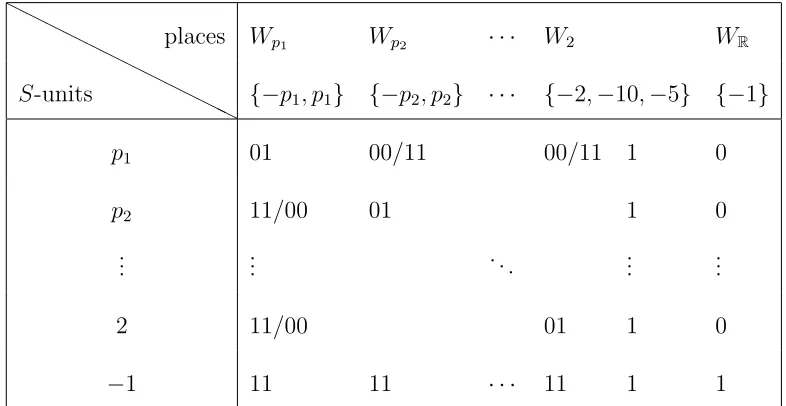
Proof. Part (a) of the theorem follows from part (b). (b) follows from theorem 4.1.4 which proves a more general situation. However, since everything about Construc-tion _Qis so concrete, part (b) can also be seen from Table 3.1. We explain the table as follows:

Z∗S is the subgroup of Q

∗ _{generated by −1,2, p}

1, . . . , pn−2. When p is odd, a

rational integer l which is prime to p is a non-square in _Q∗_p if and only if l is a non-square mod p. When l is a non-square in _Q∗_p, the corresponding image in Wp

is (1,1). Whenl is a square in_Q∗_p, the corresponding image is (0,0).

The image of Φ(_Z∗_S) in W is the matrix indicated in Table 3.1. In this table there are three entries under W2 because Q∗2/(Q

∗

2)2 is a three dimensional vector

space over _F2. The entries for a given row in the matrix are the diagonal images from a global S-unit, which is listed to the left of the row.

We will view then×2n binary matrix M in Table 3.1 as an n×n block matrix ˜

M, where each block is a pair of elements (a2i, a2i+1). Properties of this matrix ˜M

is summarized as follows:

(1) The bottom row of ˜M has all entries equal to (11).

Table 3.1: A boxed code

H H

H H

H H

H H

H H

H H S-units

places Wp1 Wp2 · · · W2 WR

{−p1, p1} {−p2, p2} · · · {−2,−10,−5} {−1}

p1 01 00/11 00/11 1 0

p2 11/00 01 1 0

..

. ... . .. ... ...

2 11/00 01 1 0

−1 11 11 · · · 11 1 1

(3) The diagonal elements of ˜M are all (01) except for the final diagonal entry, which is equal to (11).

(4) All other pairs in ˜M are either (00) or (11), which we will callidentical pairs.

We say that a block matrix having properties (1) - (4) ishalf-boxed. We will say that ˜M is boxed if the following is also true:

(5) For all (n−1)≥i > j ≥1,bij +bji = (11).

By definition, a boxed matrix has rank n and its rows are orthogonal to each other in the Euclidean pairing. Thus it is a generator matrix for a binary self-dual code.

reciprocity. Thus part (b) in theorem 3.3.1 is proved.

There is also a partial converse to the above statement, whose proof we omit:

Lemma 3.3.2. IfM˜0 is half-boxed, and its row vectors are orthogonal to each other, then condition (5) is automatically satisfied, i.e. M˜0 is boxed.

Now we proceed to prove part (c) of theorem 3.3.1.

We begin by saying the word of all-ones (denoted ¯1) belongs to every binary self-dual code C, since ¯1 is orthogonal to all vectors of even weight. Suppose now that M is the generator matrix of a self-dual code C of length 2n and that the last row of M is ¯1. Observe that elementary row operations on M correspond to a change of basis for the code C. Column permutations send C to an equivalent code. We will show by induction on n that after applying a sequence of elementary row operations and column permutations to M, one can make the associated block matrix ˜M into half-boxed form. We will in fact show that this can be done without ever adding another row to the final row ¯1 ofM. This will prove the theorem, since the above operations lead to codes equivalent to C by definition.

Forn = 2 our claim is obvious. Now suppose n >2, M is the generator matrix for a self-dual code C of length 2n and that the last row of M is ¯1. As the rows of

M have full rank, the top row is neither all-zeros ¯0 nor ¯1. Therefore the columns of M can be permuted so that the pair on the upper-left corner of ˜M is (01). M˜

has the following form:

block-Table 3.2: Block form of ˜M

01 u

w M0

vector with the same number of pairs, and M0 ∈ M at(n−1)×(2n−2). By adding the

top row of ˜M to the j-th row if necessary, where 2 ≤ j < n, we can assume that

w consists only of identical pairs. Under this hypothesis, it is easy to check that

M0 represents a generator matrix of a self-dual code of length 2n−2 with ¯1 in the bottom row. By the induction hypothesis, M0 can be turned into half-boxed form by applying column permutations and row operations while keeping the bottom row. These same operations can be applied to the augmented matrix M, leading to a matrix whose lower right cornerM0 is in half-boxed form; the column block-vector

w consists of identical pairs; the bottom row of ˜M remains ¯1.

upper-left corner of M is 10, it can be turned into 01 by permuting the first two columns of M. The block matrix ˜M is now in half-boxed form. Moreover, it is in fact boxed by lemma 3.3.2.

To complete the proof of (c), we only need to show that every boxed matrix ˜M

can be realized by the Hilbert code associated to some set S ={2,∞, p1, . . . , pn−2}.

To specify the odd pi we begin by requiring their classes in Q∗2/(Q

∗

2)2×R

∗_/(

R∗)2 as

in the last two block columns of ˜M. This can be done withpi congruent to 3 mod

4. We now choose the pi sequentially be requiring their residue classes mod pj for

1≤j < i≤n−2 according to the entrybij in ˜M. After this we have specified the

lower triangular part of a boxed matrix. By Gauss’s quadratic reciprocity, the image of these S-integers actually give a boxed matrix ˜M under our basis for the Hilbert symbols. Moreover, by the equidistribution of prime numbers in congruence classes, each self-dual code can be realized by this construction with an infinite number of distinct sets of places S.

Example 3.3.3. When S ={∞,2,3,7}, one gets the Hamming code A8. When

S ={∞,2,7,19,31,131,179,367,883,1223,1307,39079}

one gets the Golay code G24. 4

Remark 3.3.4. to be modified:

in the topological context. In the following, we will assume that all involutions that we talk about reverse the orientation on an orientable manifold. Recall to prove every self-dual code can be realized by an involution on an orientable 3-manifold with isolated fixed points, a cobordism calculation involving Ω2((RP∞)r) is used in

[KP08]. The proof proceeds by showing that certain embedded surfaces in (_RP∞)r is the boundary of an embeddable 3-manifold. This is an existence proof. Thus to find explicit examples realizing the corresponding 3-manifold remains an interesting question. We remark that while boxed-matrix descriptions of codes may not be directly useful in finding involutions on 3-manifolds with isolated fixed points, it readily describes the situation when the components of the fixed loci are circles. In the quotient of the manifold by involution, there is an orbifold-neighborhood around each fixed circle whose boundary is a 2-dimensional non-orientable surface. Actually, for odd p ≡ 3 mod 4 the “´etale surface” Spec(_Qp) is in analogy with a

Klein bottle, see section ?? for more discussions. Therefore, given a boxed-matrix, it is hopeful that we will use surgery to find a 3-manifold with an involution whose fixed loci are circles that realizes this box-matrix. This then gives the code.

3.4

A Random Generation Algorithm

The analysis of the previous section hints at an algorithm to generate all equivalence classes of binary self-dual codes of any fixed length 2n. Namely, one can assign identical pairs bij in a block matrix ˜M for 1 ≤ i < j ≤ n−1. Then ˜M can be

completed to a boxed matrix which gives a binary self-dual code. Since the pairs

bij for 1 ≤i < j ≤n−1 can be either (11) or (00) freely at will, the algorithm can

either exhaust all the 2n

2_−n

2 possibilities, or it can decide b_ij by a coin tossing. The

advantages of both algorithms are that they are not recursive on n.

The hard work remains, of course, to count the weight distribution of the codes generated; or to determine if two codes generated in this way are equivalent or not. Due to the exponential complexity in these two problems, we are more interested in the random algorithm than the exhaustive one. In fact, the random algorithm can quickly generate non-trivial (i.e. not a direct sum of codes of smaller length), or theoretically every binary self-dual codes of length 2n.

If one is only interested in codes of small length (2n ≤ 60), then the existing recursive algorithms mentioned in section 2.2.1 are appropriate. As toy examples, we also generated all binary self-dual codes of length less than 26 by implementing the random algorithm in MATLAB. For simplicity, we count the weight distribution of each outcome and compare it with the known table. The random generation process terminates when all codes in the table are obtained.

lattices as stated in [KKM91], our algorithm also gives a quick way to construct a

class of unimodular lattices. ♦

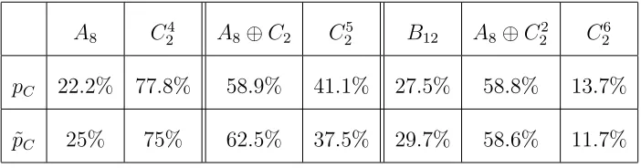
Interesting questions arise in the random generation algorithm. Suppose we assign the identical pairs bij by independently tossing a coin, then what is the

probability of generating a certain equivalence class of codes? Suppose we assign the pair to be (11) when the coin tossing produces a head. The probability of producing a head by the coin is θ. When θ = 1₂ and n is small, experiments show that this probability is very close to the true densitiespC of the equivalence classes

in T2n defined in equation 2.2.2.

In fact, denote the set of binary self-dual codes that have a boxed generator matrix by D2n. We can define the “boxed density” ˜pC of an codes equivalent to C

by

˜

pC =

|CE ∩D2n|

|D2n|

Table 3.3 compares pC and ˜pC for codes of length 8, 10, 12 where we adopt

notations for certain codes of small length in [Ple72]

Table 3.3: Comparison of densities in length 8, 10, 12

A8 C24 A8 ⊕C2 C25 B12 A8⊕C22 C26

pC 22.2% 77.8% 58.9% 41.1% 27.5% 58.8% 13.7%

˜

pC 25% 75% 62.5% 37.5% 29.7% 58.6% 11.7%

˜

pC would require a non-trivial amount of work. Therefore, for each length, we run

a Monte-Carlo simulation by letting MATLAB randomly generate 10000 codes and count the frequencies that each equivalence class shows up:

Table 3.4: Comparison of densities in length 18

H18 F16⊕C2 I18 D14⊕C22 B12⊕C23 A8⊕C25 · · ·

pC 47.30% 26.60% 12.16% 8.69% 3.55% 0.76% · · ·

˜

pC 48.97% 26.18% 11.71% 8.45% 3.18% 0.64% · · ·

Table 3.5: Comparison of densities in length 20

R20 M20 H18⊕C2 S20 F16⊕C22 I18⊕C2

pC 35.03% 23.65% 17.52% 9.85% 4.93% 4.50%

˜

pC 36.19% 23.91% 17.02% 10.12% 4.66% 3.59%

L20 D14⊕C23 K20 B12⊕C24 · · ·

pC 2.14% 1.07% 0.66% 0.33% · · ·

˜

pC 2.34% 1.08% 0.57% 0.29% · · ·

In both Table 3.4 and 3.5, we did not complete the list when pC and ˜pC gets

small. It can already be seen from the three tables that the proximity of pC and

˜

pC does not seem a coincidence. Based on proposition 2.2.2, most codes have pC

equals to (2_|Tn)!

Question 3.4.2. When n→ ∞, what is the behavior of ˜pC for most codes of length

2n?

On the above we have only considered random generation of codes based on a fair coin tossing, when experiments show that ˜pC is quite close to pC. However,

we can also use a biased coin with probability θ of producing a head, and denote the corresponding probability by ˜pθ,C. An easy observation is that given a boxed

matrix M, one may modify the first n −1 rows by adding the bottom row ¯1 to them. Thus we have a simple observation:

Proposition 3.4.3.

∀C, p˜θ,C = ˜p1−θ,C

Other than proposition 3.4.3, the general behavior of pθ,C is completely open.

For example, one may ask does θ = d2n

2n give a higher probability of producing

extremal codes than θ = 1₂? In general, we propose the following question:

Question 3.4.4. Is there a function θ(n), such that for codes of length 2n, using a biased coin with probability θ(n) for a head will most likely to produce extremal codes?

Chapter 4

Construction G

In Chapter 4 and 5 we shift gears and mainly consider questions of an arithmetic nature that arise in the search for binary self-dual codes. We will see that general duality statements give rise to possibilities of constructing codes using the arith-metic information over quite general schemes, but surprisingly even some basic questions have not been answered by the literature.

4.1

Arithmetic Duality

In appendix C we recall some glossary of derived category of bounded complexes of sheaves of R modules on the small ´etale site Xet, denoted Db(X, R). R is a ring or

a field.

Let K be a global field of characteristic different from 2. When v is a place of

K , the completion of K atv is denoted Kv. If K is a number field, let OK be the

ring of integers of K and let X = Spec(OK). If K is a function field, let X be a

smooth projective curve with function field K.

Consider F ∈ Db(SpecKv). When v is real, Kv = R. We will consider the

reduced cohomology group H_red∗ (Kv,F) := HT∗(Z/2,F); in other words, it is the

Tate cohomology groups of the Gal(_R) = _Z/2 module F. When v is not real, we will consider the usual ´etale cohomology groupH_et∗(Kv,F). In the following we will

abuse notation and write H_et∗(Kv,F) for all v. For an open subscheme U ⊂ X,

denote H_c∗(Spec(OK),F) the cohomology group with compact support, defined by

Milne [Mil06, section II.2]. S =S∞tSf is a set of places of K, whereSf contains

the places determined by the primes in the complement ofU;S∞contains all of the real places of K.

Remark 4.1.1. There are slightly different definitions of cohomology group of com-pact support in the literature, which are only different in the treatment for the real

places. ♦

[Mil06, Prop II.2.3(a)]:

· · ·H_cr(U,F |U)→Hr(U,F)→

X

v∈S

Hr(Kv,FKv)→H

r+1

c (U,F |U)· · · (4.1.1)

In arithmetic geometry, Artin-Verdier duality on arithmetic schemes [Mil06, section II.3] is the natural analogue of Pioncar´e duality on topological manifolds. Denote by µ2 the sheaf of second roots of unity. If Sf contains all places of residue

characteristic 2, then for any F ∈Db(U,_Z/2) there is a duality Theorem 4.1.2 (Artin-Verdier).

H_etr(U,Hom(F, µ2))×Hc3−r(U,F)→H

3

c(U, µ2)∼=Z/2 (4.1.2)

is a perfect duality of _F2 vector spaces.

This duality can be “lifted” to be a duality for cohomology groups of schemes over X. Let π :Y →X be a flat, projective, geometrically connected morphism of relative Zariski dimension d, d≥0. Assume Y has good reductions outside S. For

F ∈ Db_{(Y), denote the total direct image by RπF ∈ D}b_{(X). By the Leray spectral}

sequence, Hj_{(Y,F) = H}j_{(X, RπF) for all j. When i : D → X, denote the base}

change ofY overDbyYD. We will abuse notation and writeF for its pull-back on

YD.

The proper base change theorems for torsion sheaves [Mil80, Cor IV.2.3] says that in the Cartesian square:

YD i −−−→ Y πD   y π   y

D −−−→i X

If F ∈ Db_(Y,

Z/2), we have RπDi∗F = i∗(RπF) in Db(D). Thus there is no

ambiguity to define H_ci(YU,F) := Hci(U, RπF).

By assumption, YU is regular over U. There is a canonical isomorphism in

Db_(U,

Z/2) [AGV73, XVIII Th 3.2.5],

HomU(RπF, µ2)∼=RπHomYU(F, µ

⊗d+1

2 )[2d] (4.1.4)

Therefore canonically

H2d+r(YU,Hom(F, µ⊗2d+1)) =H

r_(Y

U,Hom(F, µ⊗2d+1)[2d])

=Hr(U, Rπ∗Hom(F, µ⊗₂d+1)[2d]) =Hr(U,Hom(Rπ∗F, µ2))

where the second equality is by the Leray spectral sequence; the third equality is by equation 4.1.4. Combining this with the duality H_c3−r(U, RπF) =H_c3−r(YU,F),

we get the following duality statement.

Proposition 4.1.3. The cup product pairing:

H2d+3−r(YU,Hom(F, µ⊗2d+1))×H

r

c(YU,F)→Hc2d+3(YU, µ⊗2d+1)∼=Z/2 (4.1.5)

is a perfect duality of _F2 vector spaces.

Again by the Leray spectral sequence, equation 4.1.1 translates into a statement on Db_(Y,

Z/2):

· · ·H_cr(YU,F)→Hr(YU,F)→

X

v∈S

Hr(YKv,FKv)

δr

−→H_cr+1(YU,F)· · · (4.1.6)

Since 2 is invertible on U and hence on YU, the Tate twistµ⊗2i can be identified

Proposition 4.1.4. The image of the restriction homomorphism

Φ : H_etd+1(YU, µ2)→ ⊕v∈SHetd+1(YKv, µ2)

is its own orthogonal complement with respect to the non-degenerate bilinear product

⊕v∈SHetd+1(YKv, µ2)

× ⊕v∈SHetd+1(YKv, µ2)

→ ⊕v∈SHet2d+2(YKv, µ2)

δ2d+2

−→H_c2d+3(YU, µ2)∼=F2 (4.1.7)

which is the cup product pairing composed with the boundary map in equation 4.1.6.

In 4.1.7, δ2d+2 amounts to taking summations.

Proof. We will prove the proposition in several steps.

For each placev ∈Sf, the local duality statement says that forF ∈ Db(SpecKv,Z/2),

Hi(Kv,F)×H2−i(Kv,Hom(F, µ2))→H2(Kv, µ2) =Z/2

is a perfect duality for _F2 vector spaces. (When v ∈ S∞ the statement is trivially true, in the following we will assume v ∈ S.) By arguments similar to proposition 4.1.4, we have that for F ∈ Db_(Y,

Z/2),

Hi(YKv,F)×H 2d+2−i

(YKv,Hom(F, µ

⊗d+1

2 ))→H

2d+2

(YKv, µ

⊗d+1

2 )

is a perfect duality of _F2 vector spaces. In our setting, we will take F = µ2 and

ignore all the Tate twists.

We refer to [Mil06, II.2] for the proof that in 4.1.7, δ2d+2 amounts to taking

Now we prove that the image of

Φ : H_etd+1(YU, µ2)→ ⊕v∈SHetd+1(YKv, µ2)

is its own orthogonal complement with respect to the product in 4.1.7. This is a pretty standard exercise in linear algebra. For ease of notation, denote A =

H_etd+1(YU, µ2), B = ⊕v∈SHetd+1(YKv, µ2) and C = H 2d+2

c (YU, µ2). The pairing in

equation 4.1.7 identifies the dual ˇB = Hom_F2(B,_F2) of B with B. The perfect

pairing A×C →_F2 in 4.1.5 identifies ˇA with C. From 4.1.6 for r=d+ 1 we have an exact sequence

A−→Φ B−→Ψ C (4.1.8)

Here the above pairings identify the map Ψ : ˇB →B →C= ˇA with the dual ˇΦ of Φ. Hence

dim(coker(Φ)) = dim(ker( ˇΦ)) = dim(ker(Ψ)) = dim(image(Φ))

where the last equality follows from equation 4.1.8. Thus dim(image(Φ)) = 1₂dim(B). So if we can show image(Φ) is self-orthogonal, it will be its own orthogonality complement since the product 4.1.7 is non-degenerate. We have the commutative diagram:

A×A −−−→ H2d+2_(Y

U, µ2)

  y

  y

B×B −−−→ ⊕v∈SH2d+2(YKv, µ2)

(4.1.9)

But the composition of the maps

H2d+2(YU, µ2)→ ⊕v∈SH2d+2(YKv, µ2)→H 2d+3

is 0 by the exactness of the sequence.

The construction in Proposition 4.1.4 works in complete generality. Let’s look at two examples when the relative dimension d= 0.

Example 4.1.5. When d= 0, Y =X−→Id X = Spec(OK). By the Kummer sequence

one has

O_K,S∗ /2→H1(U, µ2)→P ic(U)[2]

Thus when P ic(U) is odd, thenO∗

K,S/2 =H1(U, µ2). the image of Φ in proposition

4.1.4 is still the diagonal image Φ : O∗

K,S/2 → ⊕v∈SKv∗/2 as in Construction Q.

The cup product H1_(K

v, µ2)×H1(Kv, µ2)→Z/2 is precisely the Hilbert pairing.

However, whenP ic(U)[2] 6= 0 then the two-torsion elements in the Picard group

also come into play. 4

Example 4.1.6 (Local-Global Codes). Consider K to be the global function field

Fq(T), whereqis a prime power andq≡3 mod 4, T is a transcendental parameter.

Y = X = _P1

Fq. Let S = { 1

T, g1(T),· · ·, gn−1(T)} where each gi(T) is a monic

irreducible polynomial in _Fq[T]. Then the image of Φ is also given by the global S

-units h−1, g1(T),· · · , gn−1(T)iinW =⊕v∈SKv∗/(Kv∗)2. Moreover, when eachgi(T)

is of odd degree, then the Hilbert symbol pairing W ×W →_F2 is Euclidean. It is not hard to see that the diagonal image of Φ is also described by a boxed-matrix.

For simplicity, let’s take gi(T) = T − ai where ai are distinct integers in Z.

Suppose q > maxi|ai|, then each gi(T) will give a distinct rational point on P1_Fq.

by the Jacobi symbol (ai−aj

p ). By quadratic reciprocity, the Jacobi symbol is also

determined by the congruence conditions of q mod the prime factors in (ai−aj).

Assume (ai −aj) have distinct prime divisors when 1 ≤ i < j ≤ n −1. If we

let the primes in the congruence class of 3 mod 4 grow by magnitude, by the equidistribution of primes in congruence classes, the probability that S generating a certain equivalence classes of length 2n is the same as the random algorithm in

section 3.4 using a fair coin! 4

4.2

The Quest for Euclidean Form

The reader will have noticed that the only thing that is not addressed in propo-sition 4.1.4 is the condition when the bilinear product 4.1.7 is a Euclidean form. When it is so, then upon fixing a basis, image(Φ) becomes a self-dual code.

Recall theorem 3.2.1, a non-degenerate symmetric bilinear producth,ionW/_F2

is Euclidean if and only if ∃x, such thathx, xi= 1.

When d = 0 the question is easy. By corollary 3.2.2, when a field k has k∗/2 finite, the Hilbert pairing is Euclidean if and only if √−16∈k∗. By remark 2.2.1, a Euclidean basis fork∗/2 is unique up to permutation if and only ifdim_F2(k

∗_/2)≤3.

When K/_Q is a finite Galois extension, dim_F2(K_v∗/2) ≤ 3 for every v ∈ S if and only if the prime 2 splits completely in K/_Q. (The reader is referred to [Neu99, Proposition 5.7, Chap II] for the structure of K_v∗/2 for local fields Kv.)

When d = 1, suppose Y is a flat projective curve over Spec(OK), regular over U.

The Hochschild-Serre spectral sequence can be used to calculate Hr(YKv, µ2): Hi(Kv, Hj(YKv, µ2))⇒H

i+j_(Y

Kv, µ2) (4.2.1)

where Kv denotes an algebraic closure of Kv. This spectral sequence is

multi-plicative, where the multiplication is compatible with the cup product structure in cohomology. However, the spectral sequence along often does not suffice to deter-mine whether the product onH2(YKv, µ2) =: W is Euclidean or not, as is shown in

the following example:

Example 4.2.1 (Non-Example). SupposeYKv is the projective lineP 1

Kv. The spectral

sequence 4.2.1 degenerates on the E2 page. Denote H2,0 =_Z/2,→W generated by

{y} as an _F2 vector space. In the multiplicative spectral sequence, y2 _{∈ H}4,0 _{= 0}

for the dimension reason. Moreover, H1,1 _{= 0;H}0,2 ₌

Z/2 also pairs trivially with

itself for the same dimension reason. By the short exact sequence

0→H2,0 →W →H0,2 →0

Does it mean the cup product on W is necessarily hyperbolic?

SupposeW ={x, y}is spanned by two elementsx,y additively over_F2. H0,2 ₌

{x¯} ∈ W/{y} is a quotient space of W. The multiplicative structure on H0,2 _is

naturally induced from W as a quotient space. Since h,i is non-degenerate on W,

hy, yi= 0 implieshx, yi= 1 is non-trivial. Thus on the quotient space

Therefore the cup product hx,¯ x¯i = 0 bears no information on hx, xi. We are unable to conclude whether the product onW is Euclidean or not from the spectral

sequence 4.2.1. 4

In the topological category, product structures on the cohomology are used as a ubiquitous invariant for topological manifolds. It is very natural to explore this similar structure as an invariant for arithmetic schemes. In the arithmetic situation, when a base scheme (say SpecOK or SpecKv) containsn-th roots of unity, the sheaf

µn is canonically isomorphic to Z/n. When X is a scheme over such a base, the

cup product pairing

Hi(X, µn)∪Hj(X, µn)→Hi+j(X, µ2n)∼=Hi+j(X, µn)

makes H∗(X, µn) a ring. It is natural to ask what kind of information is encoded

in the product structure.

In our discussion on the Hilbert symbols for a local field in section 3.2, the cup product H1₍

Qp, µ2)∪H1(Qp, µ2) depends on the congruence condition p mod 4.

One can ask the following question:

Question 4.2.2. How does the congruence condition on p affect the cup product structure on H∗(_P1_Qp, µ2), or H∗(E_Qp, µ2) whereE is an elliptic curve?

Chapter 5

Equivariant Construction

Ever since the 1950s and 60s, equivariant cohomology has been a powerful tool in the study of group actions on manifolds and schemes alike. Pioneers in the field include Borel, Bredon and Grothendieck, to name a few. On the large scale, the equivariant machinery in both the topological and the arithmetic category can be stated using Grothendieck’s language of homological algebra. Some technical differences remain, of course. In the topological category, theorems in equivariant cohomology are often proved in the homotopy category of finite CW-complexes. Statements are often broken down to the “cellular level” and then “glued together”. However, in the arithmetic category it is in general more difficult to work with the ´

etale homotopy theories.

“Smith-type inequality” by invoking a result of Morin (theorem ??). In section ?? some examples are provided where the Smith type inequalities become equalities, which are the most convenient case from the point of view of constructing codes.

The goal of this chapter is two-fold: in ?? we answer question ?? by showing the pairing is hyperbolic; in ?? we provide yet one more possible construction of binary self-dual codes, which is analogous to ??.

5.1

Borel’s Equivariant Cohomology

In this section we recall Borel’s construction of equivariant cohomology. Consider a finite group G action on a complex of k-modules C∗, where k is a field. We will denote C∗ as a object in δgk[G]-Mod, where δ : Ci → Ci+1 means the differential in the complex; g refers to the fact that the complex is graded; k[G] means the complex is a module for the group ring k[G]. We refer the reader to [AP93] for a more thorough treatment.

Take a free resolution E∗ :=W∗⊗k[G] of the trivial G-modulek,

E∗ →k →0

whereE∗ is a complex

· · · Ei → Ei−1· · · → E1 → E0

The group cohomology ring of H∗(G, k) can be computed by the complex

H∗(G, k) = H∗(Homk[G](E∗, k))

It is well known that when G ∼= Z/2 and char k = 2, H∗(G, k) ∼= k[t] where deg(t) = 1. In the following, for simplicity we will assume char k = 2 whenever

G=_Z/2.

For a δgk[G]-ModC∗, denote

β_G∗(C∗) := Homk[G](E∗, C∗)

The equivariant cohomology ofC∗ is defined to be the cohomology of this com-plex,

H_G∗(C∗) := H∗(β_G∗(C∗))

This was historically called Borel’s construction of equivariant cohomology when

C∗ was the equivariant singular cochain complex of a CW complex.

We will further assume thatC∗ carries aδgk[G] morphism C∗⊗C∗ →C∗ which induces a cup product structure on H∗(β_G∗(C∗)).

Remark 5.1.1. We will denote the dual complex of E∗ as E∗ := Homk[G](E∗, k[G]). When C∗ is bounded from below, there is an isomorphism

β_G∗(C∗) =C∗⊗k[G]E∗(G)

It is often convenient to write C∗ ⊗k[G]E∗(G) ∼= C∗⊗eW

∗_{, where the twisting}

e

⊗ implies that the derivation and multiplication of the tensor productC∗⊗eW ∗ _are

not the component-wise operations on each factor. In fact, they are “twisted’’ by the k[G]-Mod isomorphism C∗⊗k[G]E∗(G)∼=C∗⊗W∗.

In this chapter we will not seek to state our results in the most general context. For the purpose of constructing codes, we will mainly focus on the special case when

G = _Z/2 is the group of order 2. In this case, the following lemma gives a better description of the δgk[G]-Mod β_G∗(C∗):

Lemma 5.1.2. [AP93, Proposition 1.3.4] Suppose G∼=Z/2, then

1. As a right k[t]-module, β_G∗(C∗)∼=C∗⊗k[t].

2. The twisted differentialδ˜isk[t] linear, where the differential onk[t] is trivial. 3. In particular, when C∗ =k, β_G∗(k)∼=H∗(β_G∗(k)).

Lemma 5.1.2 (1) says that multiplication by t is not twisted. Thus β_G∗(C∗) is a torsion-free module over k[t]. Since k[t] is a P.I.D., a torsion-free module is also a free module.

5.2

Equivariant Etale Sheaves

[AGV73][Mor08]. F is a sheaf on Xet. A G-linearization of F is a family of

mor-phisms ϕσ,:σ∗F → F indexed by σ ∈Gthat satisfy the following conditions:

• ϕ1 =Id.

• ϕτ σ =ϕτ ◦τ∗(ϕσ).

A G-linearized sheaf F is called an equivariant G-sheaf, F ∈ Sh(X, G). A morphism of G-sheavesα :F → L onXet is a morphism of sheaves that commutes

with the linearizations on F andL. In other words, if we define the action ofG on

HomSh(X)(F,L) by

σ(α) :=ϕL,σ◦σ∗(α)◦ϕ−F1,σ

Then HomSh(X,G)(F,L) is the invariant subgroup of this action.

Sh(X, G) is an abelian category with enough injectives. When F is an inject object in Sh(X, G), Γ(F) is an injective_Z[G]-Mod, [Gro57, Lemma 4.3.1].

Given a sheaf of k-modules F ∈ Sh(X, G) (k is a field), take an injective res-olution I∗ _{on X}

et and apply the global section functor, this gives a complex of

k[G]-modules:

0→ F(X)→ I0_{(X)→ I}1_{(X)· · ·}

The complex I∗_(X):

is a complex of injective k[G]-modules. Apply Borel’s construction on this complex

I∗_{(X): take a free resolution E}

∗ of the trivial modulek, define

β_Gn(F) :=T otnHom(E∗,I∗(X)) = ⊕i+j=nHomk[G](Ei,Ij(X))

The equivariant sheaf cohomology is defined as:

H_G∗(X,F) :=H∗(β_G∗(F))

The reader will also recognize this as Grothendieck’s equivariant cohomologyH∗(X, G,F), which are the derived functors of Γ(F)G_{. The above double complex construction}

just computes the derived functors of this composite functor–it is the composition of the global section functor followed by theinvariant under G functor.

In [Mor08] a modified equivariant ´etale cohomology is introduced. Consider a complete resolution J∗ of the trivialG module k,

Define

b

β_Gn(F) := T otnHom(J∗,I∗(X)) = ⊕i+j=nHomk[G](Ji,Ij(X))

b

H_G∗(X,F) :=H∗(βb_G∗(F)) Similar to lemma 5.1.2, when G=_Z/2, we have

Lemma 5.2.1. As a δgk[G]-Mod, β_G∗(F)∼=I∗ e

⊗k[t,1_t], where multiplication by t is linear; the derivation eδ is also linear on t.

• βb_G∗(k)∼=k[t,1

t] where the differentialδon the later is trivial. This induces the

familiar fact that Hb∗(G, k) = k[t,1_t] by passing to cohomology.

• βb_Gi+1(F)∼=βb_Gi(F)⊗_k[t,1

t]t.

• Hb_Gi+1(X,F)∼=Hb_Gi(X,F)⊗_k[t,1

t]t.

• Hb_G∗(X,F) is a freek[t,1_t] module.

♦

The following observation is also straight-forward, but we state it separately due to its relevance in later discussions:

Proposition 5.2.3. As a free δgk[t]-Mod,

β_G∗(F)⊗k[t]k[t,

1

t]

∼

=βb_G∗(F)

Both H_G∗(X,−) and Hb_G∗(X,−) satisfy the usual properties as a cohomological functor. For example, a short exact sequence of G-sheaves

0→ F1 → F2 → F3 →0

leads to a long exact sequence of cohomological groups in both functors. Moreoever, there are functorial spectral sequences abutting to these functors, whose E2 pages look like:

Hp(G, Hq(X,F))⇒H_Gp+q(X,F) (5.2.1) b

Hp(G, Hq(X,F))⇒Hb

p+q

G (X,F) (5.2.2)

5.3

The Localization Theorem

In topology, the classical Localization theorem relates the equivariant cohomology of a manifold to that of its ramification loci [AP93, Theorem 3.1.6]. In the ´etale context, similar results have been obtained in a recent paper [Mor08], which we briefly recall in the following.

Let X be a connected, locally Noetherian scheme. A finite group G action on

X is called admissible if X is covered by a collection of affine opens which are invariant under G, and that every orbit ofG is contained in an affine open. Under this condition, the quotient schemeX/Gcan be defined. When theG-action is free, the quotient map π:X →X/G=:W is an ´etale G-cover. We sayF ∈Sh(X, G) is adapted if ∃n, ∀V on Wet, Hq(V, πG∗F) = 0 whenq≥n+ 1. For example, when W is a regular quasi-projective scheme over_Z, and F is a locally constructible torsion sheaf, then F is adapted.

Remark 5.3.1. When theGaction onX is free,H_G∗(X,F)∼=H∗(X/G, π∗F). When the action ofG onX is trivial andF is a constant sheaf,H_G∗(X,F)∼=H∗(X,F)⊗

H∗(G,F). ♦

When the G-action on X is not free, denote by Z ⊂ X the closed sub-scheme where the inertia group is non trivial, i.e. Z the ramification locus in the coverX →

X/G =: W. Denote X0 the open complement of Z in X. An ´etale neighborhood of Z in X is an ´etale affine-morphism φ : U → X such that U ×Z X → Z is an

If φ : U → X is a G-equivariant ´etale neighborhood of Z and that φ−1_(Z)

intersects each connected component of U non-empty, then U is called a G-´etale neighborhood of Z inX. Denote Zeby the projective limit of the G-´etale neighbor-hoods of Z in X. Denote the canonical embedding i:Z →X,ei:Ze→X.

Remark 5.3.2. Suppose Z is contained in an open affine scheme SpecA, where Z

is defined by a radical ideal I. Denote (A,e Ie) the Henselization of the pair (A, I),

then Ze= SpecAe. ♦

The following Theorem 5.3.3 and Corollary 5.3.5 arelocalization theorems in the scheme-theoretic setting:

Theorem 5.3.3. [Mor08, Theorem 3.10] A finite group G acts admissibly on a locally Noetherian scheme X. F ∈ Sh(X, G) and suppose that F |X0 is adapted.

Then there is an isomorphism

b

H_G∗(X,F)∼=Hb_G∗(Z,e ei ∗_F

)

When Z is affine, we can the following isomorphism [Hub93]:

Lemma 5.3.4. Suppose F is an abelian torsion sheaf on Ze, and i :Z → Ze is the inclusion,

∀n, Hn(Z,e F) =Hn(Z, i∗F)

By the functorial spectral sequence 5.2.1 and 5.2.2, when Gacts onZe, there are

isomorphisms of equivariant cohomology groups:

Corollary 5.3.5. [Mor08, Corollary 3.11] When Z is affine and F is torsion:

b

H_G∗(X,F)∼=Hb_G∗(Z, i∗F)

Using the localization theorem, we can prove a Smith type inequality on the ´

etale site of schemes. For notational convenience, given a field k, denote k1 := k[t]/(t−1) = k[t,1_t]/(t−1). k0 :=k[t]/(t). For a graded module, − ⊗k[t]k1 is an

exact functor. When k =_F2, we will still write k0 and k1 to avoid overloading the

notations.

Proposition 5.3.6. Under the hypothesis in corollary 5.3.5, and supposeG=_Z/2, ∞

X

i=0

dimkHm+i(Z,F)≤

∞ X

i=0

dimkHm+i(X,F) (5.3.1)

for any m.

Proof. For the proof of this proposition we will use the minimal Hirsch-Brown model,

β_G∗(F)∼=H∗(X,F)⊗ek[t] (5.3.2) as introduced in appendix B. Similarly, we have the minimal Hirsch-Brown models

β_G∗(F |Z)∼=H∗(Z,F)⊗k[t] (5.3.3)

b

β_G∗(F)∼=H∗(X,F)⊗ek[t, 1

t] (5.3.4)

b

β_G∗(F |Z)∼=H∗(Z,F)⊗k[t,

1

t] (5.3.5)

Since the action ofGonZ is trivial, the complex 5.3.3 has trivial differential. Thus

Define a filtration:

Fm(βG∗(F)) :=⊕ m i=0H

i

(X,F)⊗ek[t] (5.3.6)

Fm(βG∗(F |Z)) :=⊕mi=0H

i_(Z,F)⊗k[t]

The inclusion morphism i : Z → X induces a graded morphism in equivariant cohomology

i]: X

p+q=n

Hp(X,F)e⊗tq→ X

p+q=n

Hp(Z, i∗F)⊗tq

Induction on n shows that the morphism i] respects the filtration: ∀m, i] :

Fm(βG∗(F |Z))→ Fm(β∗G(F)), which fits into the following diagram

0 −−−→ Fm−1(βG∗(F)) −−−→ βG∗(F) −−−→ βG∗(F)/Fm−1 →0

i]   y i ]  

y ¯i

]

  y

0 −−−→ Fm−1(βG∗(FZ)) −−−→ βG∗(F |Z) −−−→ βG∗(F |Z)/Fm−1 →0

(5.3.7)

After localizing at⊗k[t]k1and taking cohomology, the middle mapi]⊗k[t]k1becomes

an isomorphism. Since the differential on H∗(Z, i∗F) ⊗k[t] is trivial, the map ¯_i]_⊗

k[t]k1 is surjective on the cochain level as well. Since

∞ X

i=m

dimkHi(X,F) = dimk(βG∗(F)/Fm−1)⊗k[t]k1

∞ X

i=m

dimkHi(Z,F) = dimk(βG∗(F |Z)/Fm−1)⊗k[t]k1

we get the desired inequality.

Proposition 5.3.6 can also be compared with Bredon’s equivariant cohomology of alocal system on a variety over an algebraically closed field [Sym04], which proves

the same Smith type inequality when G=_Z/2. ♦

Proposition 5.3.8. [AP93, Proposition 1.3.14] The following two conditions are

equivalent:

(a) The differentialδin the minimal Hirsch-Brown model 5.3.2 ofβ_G∗(F)vanishes; (b)

∞ X

i=0

dimkHi(Z,F) =

∞ X

i=0

dimkHi(X,F)

Proof. (a)⇒(b) is obvious.

(b)⇒(a) : Factorδinto a surjection followed by an injection: H∗(X,F)⊗ek[t]→

M → H∗(X,F)e⊗k[t]. M is a sub-module of the free k[t]-Mod β_G∗(F). When equality is reached in (b), the differential inβ_G∗(F)⊗k[t]k1is trivial. ThusM⊗k[t]k1 =

0, which implies M = 0 since M is free.

Based on proposition 5.3.8, when equality is reached, the differential on both of the minimal Hirsch-Brown modelsβ_G∗(F) ( 5.3.2 ) and β_G∗(F |Z) ( 5.3.3 ) are trivial.

In this case, H_G∗(X,F)∼=β_G∗(F) as δgk[t]-Mod. i] induces a map between two free

k[t]-Mod which is an isomorphism after tensoring with k1, this implies that i] is

5.4

Equivariant Construction

Now consider the situation in Chapter 4. Y is an integral projective scheme over Spec_Z[1₂], regular over an open sub-scheme U ⊂ Spec_Z[1₂]. The group G = _Z/2 acts onY. The constant sheafF =µ2 ∈Sh(Y, G) is adapted onY. We have

Artin-Verdier duality for the ringH∗(YU, µ2) by ignoring the Tate twists sinceµ⊗2n ∼=Z/2

onY. H∗(YU, µ2) will be called a Pioncar´e algebra, which is an algebra that satisfies

the following requirements:

An orientation on a k-algebra A is a non-trivial k-linear map:

OA:A→k

A is called a Poincar´e algebra if the multiplication in A followed by orientation

A×A →AOA

−→k induces an k-linear isomorphism A→Homk(A, k).

• Suppose A = ⊕n

i=0Ai is a graded algebra. If OA(Ai) = 0 when i < n, A is

called a graded Poincar´e algebra of formal dimension n.

• A is called a filtered algebra of formal length n+ 1 if there is a filtration

0⊂ F−1A ⊂ F0A⊂ · · · ⊂ FnA=A

which is compatible with the product FiA× FjA⊂ Fi+jA.

If OA(Fn−1A) = 0; ∀i, FiA is isomorphic to Homk(A/Fn−i−1A, k), then

Given a graded algebra A, we can associate to it a filtered algebra A, where

FmA := ⊕mi=0Ai. Conversely, given a filtered algebra A, we can associate to it a

graded algebra A :=gr(A), where Am :=Am/Am−1.

Proposition 5.4.1. [AP93, Proposition 5.1.3]A is a filtered Poincar´e algebra if A

is a graded Poincar´e algebra, and vice versa.

Thanks to Artin-Verdier duality, we have already seen that H∗(YU, µ2) is a

graded Poincar´e algebra under the cup-product. Moreover, when equality is reached in proposition 5.3.8, we have an isomorphism of _F2 vector spaces:

H∗(Y, µ2)∼=H∗(Y, µ2)⊗eF2[t]⊗_F2[t]k1 (5.4.1)

However, the multiplication structure of the algebra on the R.H.S is “twisted” from that on the L.H.S. Recall the R.H.S. has a natural filtrationFm defined in the proof

of proposition 5.3.6. We have a straight forward observation:

Lemma 5.4.2. gr(H∗(Y, µ2)⊗eF2[t]⊗_F2[t]k1)∼=H

∗_{(Y, µ}

2) as a graded algebra.

In corollary 5.3.5,i]_⊗

F2[t]k1 induces an isomorphism ofF2 vector spaces.

H∗(Y, µ2)⊗eF2[t]⊗F2[t]k1

i]_⊗

F2[t]k1

−→_∼

= H

∗

(Z, µ2)⊗F2[t]⊗F2[t]k1 (5.4.2)

Remark 5.4.3. Equation 5.4.2 is a map of filtered algebras. To distinguish the situation, we will denote the original filtration on β_G∗(Z, µ2) by Fe, i.e.

e

Fm(βG∗(Z, µ2)) = m

X

i=0

as a filtered differential algebra. Since the differential is trivial, this filtration struc-ture passes to the cohomology

e

Fm(HG∗(Z, µ2)) =

m

X

i=0

Hi(Z, µ2)⊗k[t]

One can also apply the functor⊗_F2[t]k1 to equation 5.4.3, which commutes with

taking cohomology.

On the other hand, one can also translate the filtered algebra structure from the L.H.S. of equation 5.4.2 to the R.H.S. by the vector space isomorphism. We will denote this filtered algebra structure on H_G∗(Z, µ2)⊗F2[t]k1 by F. ♦

Since theG-action on Z is trivial, the algebra structure on H_G∗(Z, µ2)⊗F2[t]k1 =

H∗(Z, µ2)⊗F2[t]⊗F2[t]k1 and H

∗_{(Z, µ}

2) are the same. One gets a filtration F on H∗(Z, µ2) by a chain of isomorphisms

H∗(Y, µ2)

gr

←−H∗(Y, µ2)e⊗F2[t]⊗F2[t]k1 ∼=H

∗

(Z, µ2)⊗F2[t]⊗F2[t]k1 ∼=H

∗

(Z, µ2)

When Y has relative dimension d over Spec_Z[1₂], Fd+1H∗(Z, µ2) becomes its

own orthogonal complement in the filtered algebra structure. When the induced bilinear product:

H∗(Z, µ2)×H∗(Z, µ2)→H∗(Z, µ2)/F2d+2 ∼=F2

is a Euclidean form,Fd+1H∗(Z, µ2) is a self-dual code. This is our third construction

of binary self-dual code, the equivariant construction.

Example 5.4.4. Suppose Y is a hyper-elliptic curve defined by y2 _{= f(x) over a}

into m irreducible factors over _Fq. Consider the double cover π : Y → P1_Fq. The

Galois group of this cover acts on Y as an involution τ. There are m+ 1 closed points which ramify in this cover: each fi(x) gives a closed point Zi of degree

di = deg(fi); and there is the point at infinity ∞. Denote their union by Z.

P∞

j=0h

j_{(Z, µ}

2) =

Pm+1

i=1

P1

j=0h

j_(Z

i, µ2) = 2(m+ 1).

Now we will compute P∞_i=0hi_{(Y, µ}

2):

• h0_{(Y, µ}

2) = 1.

• By the Kummer sequence:

0→_F∗_q/2→H1(Y, µ2)→P ic0(Y)[2]→0

Thus h1(Y, µ2) = 1 + dim_F2P ic

0_(Y)[2].

Geometrically, P ic0_(Y

Fq)[2] is generated as a group by the ramification points

of Y_Fq/_P1

Fq. ThereforeP ic

0_{(Y)[2] is generated by the divisors (Z}

i)−di(∞) for

0 ≤ i ≤ m, subject to the relation Pm

i=0(Zi)−(2g+ 1)(∞) = 0 in P ic0(Y).

Hence

dim_F2P ic

0_{(Y)[2] =m−1}

By Artin-Verdier duality forY_Fq, ∞

X

i=0

hi(Y, µ2) =

4

X

i=0

hi(Y, µ2) = 2(m−1 + 1 + 1) = ∞ X

i=0

The isomorphism H_τ∗(Y, µ2) ⊗F2[t] k1 ∼= H

∗_{(Z, µ}

2) gives H∗(Z, µ2) a filtered

Poincar´e algebra structure of length 4. The orientation in H∗(Z, µ2) is defined

by taking the quotient over F2. The question that whether the bilinear product

H∗(Z, µ2)×H∗(Z, µ2)→H∗(Z, µ2)/F2 ∼=F2

is a Euclidean or an alternate form depends on Y. When the form is Euclidean, then upon fixing a basis, the image F1(H∗(Y, µ2)⊗F2[t]k1)→H

∗_{(Z, µ}

2) is a binary

self-dual code. However, in example 5.5.4 we will see an example when this form is

alternate. 4

5.5

Comparison with Construction G

In this section, we will compare the Equivariant Construction in section 5.4 with Construction G in chapter 4. The reader is referred to proposition A.0.10 for a comparison result in the topological situation. The comparison in the arithmetic situation is more complicated though, due to the fact that a closed point on an algebraic variety YK has cohomological dimension higher than zero, when the base

field K is not algebraically closed.

Proposition 5.5.1. There is a Mayer-Vietoris sequence:

· · ·Hi−1(U ,e F)→Hi(Y,F)→Hi(U,F)⊕Hi(Z,e F)→Hi(U ,e F)· · · (5.5.1) Proof. By the long exact sequence [Mil80, proposition III.1.25]:

· · · →H_Zi(Y,F)→Hi(Y,F)→Hi(U,F)→H_Zi+1(Y,F)· · · (5.5.2) ReplaceY by Ze, one gets

· · · →H_Zi(Z,e F)→Hi(Z,e F)→Hi(U ,e F)→H_Zi+1(Z,e F)· · · (5.5.3) Now we will relate equation 5.5.2 with equation 5.5.3. Suppose Y0 is an ´etale neighborhood of Z, i.e. Y0 ×Y Z ∼= Z. There is an excision theorem [Mil80,

Proposition III.1.27]:

H_Zi(Y,F)∼=H_Zi(Y0,F)

The system of ´etale neighborhoods of Z ⊂ Y is a naturally filtered projective system. Since ´etale cohomology commutes with taking filtered projective limit of schemes, [Mil80, III Lemma 1.16]:

H_Zi(Y,F)∼= lim_−→

Y0

H_Zi(Y0,F)∼=H_Zi(lim_←−Y0,F) = H_Zi(Z,e F)

Piecing together equation 5.5.2 and equation 5.5.3, one gets the Mayer-Vietoris sequence in equation 5.5.1.

Remark 5.5.2. Comparing with the topological Mayer-Vietoris sequence, the intu-ition behind proposintu-ition 5.5.1 is that Ze is viewed as a “tubular neighborhood” of

Corollary 5.5.3. By the functorial spectral sequence in equation 5.2.1, one gets an

equivariant Mayer-Vietoris sequence:

· · ·H_Gi−1(U ,e F)→H_Gi(Y,F)→H_Gi(U,F)⊕H_Gi(Z,e F)→H_Gi (U ,e F)· · · Example 5.5.4. In the situation of example 5.4.4,F1(H∗(Y, µ2)⊗F2[t]k1)→H

∗_{(Z, µ}

2)

is its own orthogonal complement, according to the equivariant construction. The function field of Y is K. Z = tm+1

i=1 is the ramification loci in the double cover π : Y → _P1

q. Each closed point Zi corresponds to a ramified place pi of K. Zi =

Spec_Fpi where Fpi is the residue field of the valuation at pi. Zei = SpecO

a

K,pi where

Oa

K,pi means the algebraic elements in OK,pi, i.e. the Henselization ofOK at pi. As

far as ´etale cohomology is concerned, one can safely replace Oa

K,pi by OK,pi. Ze =

tm+1

i=1 SpecOK,pi. Denote the open complement ofZ ⊂ZebyUe. Ue =t

m+1

i=1 SpecKpi.

Denote the branch loci in _P1

Fq by Z

0_{; the open complement of Z}0 _⊂

P1Fq by A.

As reduced schemes Z0 =Z. Denote the open complement ofZ0 ⊂Ze0 byU0. Then

U0 = tm+1

i=1 SpecFq(x)pi, where pi is the restriction of the place pi on the subfield Fq(x) ⊂ K. In Construction G, the image of H1(A, µ2) → H1(U0, µ2) is its own

orthogonal complement.

Comparison of vector spaces:

This argument is similar to proposition A.0.10. By corollary 5.5.3, there is an equivariant Mayer-Vietoris sequence:

· · · →H_τj(Y, µ2)→Hj(A, µ2)⊕Hτj(Z, µe 2)→Hτj(U , µe 2)→Hτj+1(Y, µ2)→ · · ·

(5.5.4) We will show that ∀i, the map H1

τ(Ze_i, µ₂)→H_τ1(Ue_i, µ₂) is an isomorphism. By lemma 5.3.4, Hj₍

e

Zi, µ2) =Hj(Zi, µ2). Thus it is easy to see that τ reaches

the maximality condition on Ze_i. Therefore H_τ∗(Ze_i, µ₂) =H∗(Z_i, µ₂)⊗F2[t].

h1

τ(Ze_i, µ₂) = 2.

On the other hand, H1

τ(U , µe 2) ∼= H1(U0, µ2). Dimension calculation says that

the spectral sequences in equation 5.2.1 for bothH_τ1(Ze_i, µ₂) andH_τ1(Ue_i, µ₂) converge on the E2 page. We can compare the sequences:

0→H1₍

Z/2, H0(OK,pi, µ2)) −−−→ H 1

τ(OK,pi, µ2) −−−→ H 0₍

Z/2, H1(OK,pi, µ2))→0

  yd1

  yd2

  yd3 0→H1(_Z/2, H0(Kpi, µ2)) −−−→ H

1

τ(Kpi, µ2) −−−→ H 0₍

Z/2, H1(Kpi, µ2))→0

(5.5.5) It is easy to see d1 is an isomorphism.

On the other hand, H1_(K

pi, µ2) ∼= K

∗

pi/2 is generated as a group by {pi, ui},

wherepiis a uniformizer anduiis a non-square unit. However, sinceKpi/Fq(t)pi is a

ramified extension,_Z/2 acts non-trivially on the uniformizerpi. ThusH0(Z/2, H1(Kpi, µ2))

is represented by{ui}which is the isomorphic image ofd3(H0(Z/2, H1(OK,pi, µ2))).