International Journal of Industrial Engineering Computations 6 (2015) 469–480
Contents lists available at GrowingScience
International Journal of Industrial Engineering Computations
homepage: www.GrowingScience.com/ijiec
A dual response surface optimization methodology for achieving uniform coating
thickness in powder coating process
Boby John*
SQC & OR Unit, Indian Statistical Unit, Bangalore, India – 560059
C H R O N I C L E A B S T R A C T
Article history: Received May 16 2014 Received in Revised Format April 10 2015
Accepted May 20 2015 Available online May 20 2015
The powder coating is an economic, technologically superior and environment friendly painting technique compared with other conventional painting methods. However large variation in coating thickness can reduce the attractiveness of powder coated products. The coating thickness variation can also adversely affect the surface appearance and corrosion resistivity of the product. This can eventually lead to customer dissatisfaction and loss of market share. In this paper, the author discusses a dual response surface optimization methodology to minimize the thickness variation around the target value of powder coated industrial enclosures. The industrial enclosures are cabinets used for mounting the electrical and electronic equipment. The proposed methodology consists of establishing the relationship between the coating thickness & the powder coating process parameters and developing models for the mean and variance of coating thickness. Then the powder coating process is optimized by minimizing the standard deviation of coating thickness subject to the constraint that the thickness mean would be very close to the target. The study resulted in achieving a coating thickness mean of 80.0199 microns for industrial enclosures, which is very close to the target value of 80 microns. A comparison of the results of the proposed approach with that of existing methodologies showed that the suggested method is equally good or even better than the existing methodologies. The result of the study is also validated with a new batch of industrial enclosures.
© 2015 Growing Science Ltd. All rights reserved
Keywords:
Powder coating Industrial enclosures Dual response surface methodology Design of experiments Analysis of variance
1. Introduction
The industrial enclosures are cabinets used for mounting the electrical and electronic equipment. The enclosures protect the equipment from outside environment and adverse weather conditions. The enclosures can also protect the user from electromagnetic interferences (Chen et al., 2008). In many situations, only the enclosure will be visible to the users. Hence the appearance of the enclosures should be attractive to the customers. The enclosure painting process is a very important step in enclosure manufacturing process. The enclosures are generally painted using powder coating method. The powder coating, as a painting technique, does not require any solvent and is applied as free flowing dry powder. The solvent emission is considered as a major problem in surface coating industry. Hence powder coating has superior techno-economic benefits (Naderi et al., 2004). It creates a hard finish. The first step in
* Corresponding author. Tel: +91 94487 04182 Fax: +91 80 2848 491 E-mail: [email protected] (B. John)
powder coating is the preparation of the surface to be coated. This involves removal of oil, greases, etc. from the surface. The common methods for surface preparation are degreasing, etching, rinsing, etc. After the surface is prepared, it is heated and the powder is sprayed to the metal surface using an electrostatic gun. The powder melts to form a uniform film and is then cooled or cured to form a hard coating.
The coating thickness is an important quality characteristic of powder coating process. It affects the mechanical and physical properties of the coated surface. If the coating thickness is not uniform across the surface, it would impact the hardness, surface appearance and corrosion resistivity of the enclosures. A company manufacturing industrial enclosures is facing the serious problem of coating thickness variation in the powder coated enclosures. This reduced the attractiveness of the enclosures and also resulted in customer dissatisfaction. Hence this study is undertaken to develop a methodology to reduce the variation in coating thickness around the target for industrial enclosures.
The remaining part of the paper is arranged as follows. The methodology is discussed in session 2. The data collection and analysis is given in session 3. The session 4 provides the optimization details. The results are discussed in session 5 and validated in session 6. The conclusions are given in session 7.
2. Methodology
There are many approaches for achieving the target value of a response variable. Most of these approaches are based on response surface methodology (Box & Draper, 1987). Response surface methodology (RSM) is a collection of statistical and mathematical techniques for improving and optimizing processes (Mayers et al., 2009). The RSM identifies the best settings for a set of input or design variables that would optimize the response y (Box & Wilson, 1951; Sahoo et al., 2013). Lots of work, both theoretical and applied, have been carried out in the recent past in the area of response surface methodology (Khuri & Mukhopadhyay, 2010; Bezerr et al., 2008; Baş & Boyacı, 2007; Liyana-Pathirana & Shahidi, 2005; Noordin, 2004; Öktem, 2005; Barton, 2013). The main emphasis of RSM is on optimizing the estimated mean of the response variable (Ding et al., 2004). The mean is estimated using a polynomial model given in Eq. (1).
∑ ∑ < + ∑ = + ∑ = + = k j i j x i x ij a k i i x ii a k i i x i a a y 1 2 1 0 µ (1)
where yµ is the estimated value of the mean of the response y and xi, i = 1, 2, …, k, are the exploratory
variables. Using Eq. (1), the optimum values of xi’s, which would bring yµ close to the target is then
determined. But the optimum xi’s may not minimize or change the variance. In RSM and traditional
industrial experimentation, it is assumed that the variance is constant. But the assumption on constant variance doesn’t hold well in many industrial scenarios. Hence it is required to simultaneously optimize multiple responses, namely mean and variance of the response variable (Taguchi, 1986; Phadke, 1995). The most efficient methodology for simultaneous optimization of the mean and variance is dual response surface methodology (Myers & Cartel, 1973). In dual RSM, along with the model for estimating the mean of the response variable, another polynomial model for estimating the standard deviation is also developed as shown in Eq. (2).
∑ ∑ < + ∑ = + ∑ = + = k j i j x i x ij b k i i x ii b k i i x i b b y 1 2 1 0 σ (2)
where y
σ is the estimated value of the standard deviation of the response y and xi, i = 1, 2, - - -, k, arethe exploratory variables. Then both the responses (mean and variance) are optimized, simultaneously.
Several methods have been proposed for the simultaneous optimization of mean and variance of the response variable. The important among them are
• Vining and Mayers (VM) method (Vining & Myers, 1990)
• Lin and Tu (LT) method (Lin & Tu, 1995)
• Quality loss function (QLP) method (Ames et al., 1997).
In VM method, one of the responses is taken as the primary response and the other one as a constraint. The VM approach is to
min y
σ
subject to y
µ
=T (3)where yµ and yσ are estimated mean and standard deviation of the response variable y obtained using Eq. (1) and Eq. (2). T is the target value for y. Del Castillo and Montgomery (1993) showed that the VM problem can be solved using Excel solver (Brown, 2001). The Excel solver uses generalized reduced gradient algorithm for solving optimization problems. Still many researchers encountered the problem of not getting a feasible solution to the dual response optimization problem using VM method. This is because the VM method tries to find out an optimum solution which forcefully ensures the mean exactly on target.
The LT method proposes to solve the dual response optimization problem by minimizing the mean square error (MSE). The LT method is to
minMSE=(yµ −T)2+yσ2 (4)
where yµ and yσ are estimated mean and standard deviation of the response variable y obtained using Eq. (1) and Eq. (2). T is the target value for y. The problem with LT method is that it may minimize the MSE without bringing yµ close to the target T. This is because the LT method does not have an upper
limit or restriction on the deviation of yµfrom the target T.
The aforementioned problem is taken care in CN method. The CN method is to
min y
σ
subject to (yµ −T)2≤∆2,
(5)
where ∆ is the maximum allowed deviation of estimated mean yµ from the specified target value. The
CN method is considered to be logically sounder among the aforementioned three methods. But the CN method is also not free from problems. The presence of higher order polynomials in the constraint sometimes makes it difficult to obtain the global optimum solution using commonly used optimization programs like Excel solver.
An alternative approach suggested is to minimize the quality loss function (referred as QLP method). Many papers on a wide variety of applications of Taguchi’s loss function is published in the recent past (Liao & Kao, 2010; Pi & Low, 2006; Antony, 2000; Antony, 2001; Wu, 2004; Kethley, 2002; Chan & Ibrahim, 2004; Cho & Cho, 2008; John, 2012). The QLP method is to
minQLP=wµ µ(y −Tµ)2+wσ σ(y −Tσ) ,2 (6)
In this study, the author has used the CN method and the problem of higher order polynomials in the constraints is handled by slightly modifying the CN method. The methodology is a simplified version of the CN method. The step by step details of the proposed methodology is given below:
1. Identify the control variables or factors xi’s, i = 1,2, …, k.
2. Identify the important factors among xi’s which significantly influence the response variable
through design of experiments.
3. Develop the models for estimating the mean yµ and the standard deviation yσ of the response variable y.
4. Identify the optimum values of xi’s which would simultaneously optimize the mean and standard
deviation of response y by min y
σ
subject to (T−
∆
)≤y
µ
≤(T+∆
), (7)where ∆ is the maximum allowed deviation of estimated mean yµ from the specified target value T. The optimization problem (7) can be easily solved using the generalized reduced gradient algorithm of Excel solver (Fylstra et al., 1998).
3. Data collection and analysis
Through discussions with the technical personals and surface coating experts of the company four variables namely oven temperature (in 0C), curing time (in minutes), conductivity (in micro seimens) and powder output (in grams per second) of the powder coating process are identified as factors for the study. The coating thickness (in microns) is chosen as the response variable. The effect of the factors on the coating thickness is studied using design of experiments. The design of experiments is an efficient tool for optimizing the process and product characteristics (Chowdhury & Boby, 2003; Surm et al., 2005; Wang et al., 2008; Bhuiyan, 2011; Sahoo & Sahoo, 2011; Boby, 2013; Kirshna et al., 2013;, Saha & Mandal, 2013; Sahoo, 2014). Since response surfaces need to be fitted for mean and variance of the response variable, a central composite design (CCD) is chosen for experimentation (Alam et al., 2008). The central composite designs have less number of experiments compared to 3 level full factorial experiments. The CCDs are factorial experiments augmented with additional central and axial points. The factors with the levels, central points and axial points are given in Table 1.
Table 1
Factors with levels
Factor Name Code Levels Central Point Axial Points
-1 +1 0 -2 2
Oven Temperature x1 185 200 192.5 177.5 207.5
Curing Time x2 10 12 11 9 13
Conductivity x3 1500 1800 1650 1350 1950
Powder Output x4 32 34 33 31 35
The experiments are conducted as per the design and the response, coating thickness is measured. Each experiment is replicated twice. The experimental layout with the mean and variance of the response is given in Table 2. The mean of the response is subjected to analysis of variance (Box, 2009). The ANOVA table is given in Table 3.
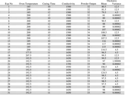
Table 2
Experimental layout with response mean and variance
Exp No Oven Temperature Curing Time Conductivity Powder Output
Thickness Mean Variance
1 185 10 1500 32 80.5 12.5
2 200 10 1500 32 81.5 12.5
3 185 12 1500 32 79.5 4.5
4 200 12 1500 32 81 8.00002
5 185 10 1800 32 89 8.00002
6 200 10 1800 32 90.5 12.5
7 185 12 1800 32 88 8.00002
8 200 12 1800 32 89 8.00002
9 185 10 1500 34 107 8.00002
10 200 10 1500 34 108.5 12.5
11 185 12 1500 34 106 8.00002
12 200 12 1500 34 107.5 12.5
13 185 10 1800 34 116 8.00002
14 200 10 1800 34 117 8.00002
15 185 12 1800 34 115 8.00002
16 200 12 1800 34 116.5 4.5
17 177.5 11 1650 33 96.5 4.5
18 207.5 11 1650 33 99.5 12.5
19 192.5 9 1650 33 99.5 12.5
20 192.5 13 1650 33 97 1.99999
21 192.5 11 1350 33 90 8.00002
22 192.5 11 1950 33 106.5 4.5
23 192.5 11 1650 31 72 8.00002
24 192.5 11 1650 35 124.5 4.5
25 192.5 11 1650 33 98.5 4.5
26 192.5 11 1650 33 97.5 4.5
27 192.5 11 1650 33 98.5 4.5
28 192.5 11 1650 33 97.5 4.5
29 192.5 11 1650 33 99 8.00002
30 192.5 11 1650 33 98 8.00002
31 192.5 11 1650 33 99 8.00002
Table 3
ANOVA table for thickness mean
Source DF SS MS F p
Regression 14 4709.28 336.38 1471.41 0.00
Linear 4 4708.96 1177.24 5149.59 0.00
Square 4 0.1 0.03 0.11 0.977
Interaction 6 0.22 0.04 0.16 0.984
Residual Error 16 3.66 0.23
Lack-of-Fit 10 1.23 0.12 0.3 0.953
Pure Error 6 2.43 0.4
Total 30 4712.94
Table 4
Coefficient table for thickness mean
Code Coefficients Standard Error t Stat P-value
Intercept -399.950269 3.561889813 -112.29 0
Oven Temp x1 0.091666667 0.010644676 8.6115 0
Curing Time x2 -0.52083333 0.079835072 -6.5239 0
Conductivity x3 0.028472222 0.000532234 53.4957 0
Residual P er ce nt 1.0 0.5 0.0 -0.5 -1.0 99 90 50 10 1 Fitted Value R es id ua l 120 100 80 0.8 0.4 0.0 -0.4 -0.8 Residual Fr eq ue nc y 0.8 0.4 0.0 -0.4 -0.8 8 6 4 2 0 Observation Order R es id ua l 30 28 26 24 22 20 18 16 14 12 10 8 6 4 2 0.8 0.4 0.0 -0.4 -0.8
Normal Probability Plot of the Residuals Residuals Versus the Fitted Values
Histogram of the Residuals Residuals Versus the Order of the Data Residual Plots for Mean
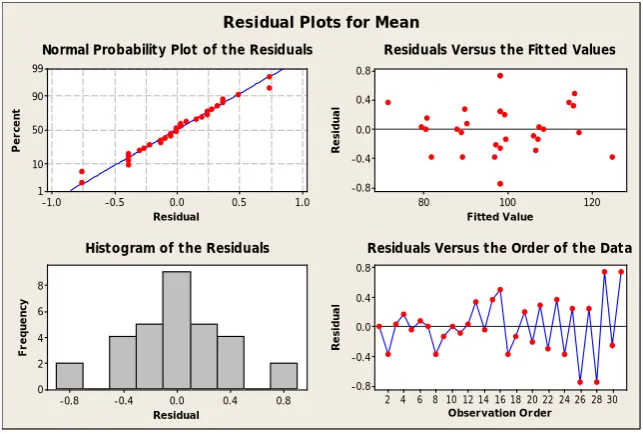
Fig. 1. Residual plots for thickness mean
The residual plot showed that the residuals are approximately normally distributed and there is no trend or pattern in the residual versus order of the data or residual versus the fitted values (Montgomery, 2012). Hence the model for the mean of the coating thickness is identified as
4 13.3125x 3 2x 0.02847222 2 x 0.52083333 -1 0.0916667 9
-399.95026 + + +
= x
y
µ
(8)Similarly the variance of the response is subjected to analysis of variance. The ANOVA table for variance is given in Table 5.
Table 5
ANOVA table for thickness variance
Source DF SS MS F P
Regression 14 198.23 14.159 2.56 0.037
Linear 4 131.04 32.76 5.92 0.004
Square 4 36.35 9.087 1.64 0.213
Interaction 6 30.84 5.141 0.93 0.501
Residual Error 16 88.6 5.538
Lack-of-Fit 10 67.6 6.76 1.93 0.217
Pure Error 6 21 3.5
Total 30 286.84
The ANOVA table shows the regression is significant (p value = 0.037 < 0.05) at 5 % level and the lack of fit (p value = 0.2176 > 0.05) is insignificant indicating that the regression model is a good fit. The coefficients of the significant factors are given in Table 6.
Table 6
Coefficient table for thickness variance
Code Coefficients Standard Error t Stat P-value
Intercept 535.3152619 294.7195892 1.81635 0.08044
Oven Temperature x1 -5.45348197 3.06295487 -1.7805 0.08626
Curing Time x2 -1.7291612 0.495350216 -3.4908 0.00167
Table 6 revealed that the factor namely curing time (x2) is significant at 5% level and the oven temperature
(x1) and over temperature2 (x12) are significant at 10% level (p value < 0.10). The residual plots are given
in Fig. 2.
Residual P er ce nt 5.0 2.5 0.0 -2.5 -5.0 99 90 50 10 1 Fitted Value R es id ua l 12 10 8 6 4 4 2 0 -2 -4 Residual Fr eq ue nc y 4 2 0 -2 8 6 4 2 0 Observation Order R es id ua l 30 28 26 24 22 20 18 16 14 12 10 8 6 4 2 4 2 0 -2 -4
Normal Probability Plot of the Residuals Residuals Versus the Fitted Values
Histogram of the Residuals Residuals Versus the Order of the Data Residual Plots for Variance
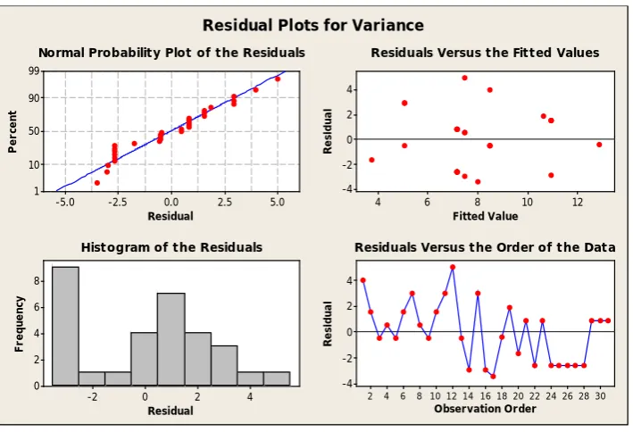
Fig. 2. Residual plots for thickness variance
The residual plot showed that the residuals are normally distributed and there is no trend or pattern in the residual versus order of the data or residual versus the fitted values. Hence the model for the variance of coating thickness is identified as
2 1 0.014591x 2 1.729161x -1 5.4534821x -535.315262
2 = +
σ
y (9)
4. Optimization
The company professionals suggested that a coating thickness of 80 microns is ideal for the industrial enclosures. Hence the thickness target is chosen as 80 with a tolerance ∆ of 0.05 microns. Substituting Eq. (8) and Eq. (9) in Eq. (7), the optimization problem became
.
min (535.315262-5.4534821x -1.729161x 0.014591x )
1 2 1
2 0 5
yσ = +
subject to 80 4 13.3125x 3 2x 0.02847222 2 x 0.52083333 -1 0.0916667 9 -399.95026 95 .
79 ≤ + x + + ≤
200 1 185≤x ≤
12 2 10≤x ≤
1800 3
1500≤x ≤
34 4 32≤ x ≤
, ,.., integer
x i 1 4
i =
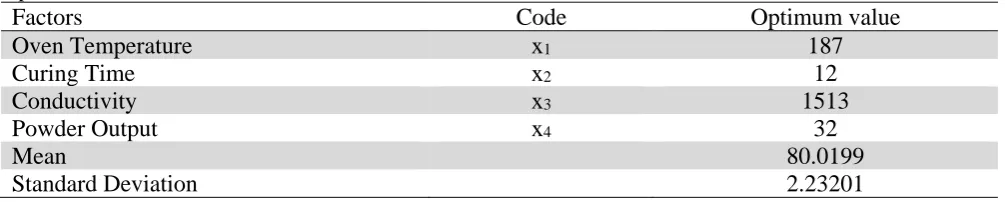
The integer constraint is added because the least count for most of the factors is one unit. The aforementioned problem is an integer programming problem (Hiller and Liberman, 2008; Taha, 2007). This problem can be solved using Excel solver. The solver uses one of the most robust nonlinear programming methods, namely generalized reduced gradient algorithm. This algorithm is developed by Lasdon and Waren (Lasdon & Waren, 1977; Lasdon et al., 1978). Moreover lot of studies have been published on the applications of MS Excel solver in solving industrial problems (Souliman et al., 2010; Dasgupta, 2008; Fang, 2006; Brown, 2006). The solution obtained is given in Table 7. The table showed that the optimum combination of factors would give an average coating thickness of 80.0199 microns, very close to the target value of 80 microns with a standard deviation of 2.232 microns.
Table 7
Optimum solution
Factors Code Optimum value
Oven Temperature x1 187
Curing Time x2 12
Conductivity x3 1513
Powder Output x4 32
Mean 80.0199
Standard Deviation 2.23201
5. Results and discussion
In this study, models are developed for estimating the mean and variance of the coating thickness of powder coated enclosures. The models are developed in terms of powder coating process parameters namely oven temperature, curing time, conductivity and powder output. Then the variation around the target value of coating thickness is minimized by simultaneously optimizing the mean and standard deviation of the coating thickness. The study showed that the optimum values of oven temperature, curing time, conductivity and powder output would give an estimated average coating thickness of 80.0199 microns, very close to the target value of 80 microns.
Table 8
Comparison of results obtained using different optimization methods
Factors Code Proposed Method VM Method LT Method CN Method QLP Method
Oven Temperature x1 187
No feasible Solution
187 187 187
Curing Time x2 12 12 12 12
Conductivity x3 1513 1513 1505 1513
Powder Output x4 32 32 32 32
Mean 80.0199 80.0199 79.7921 80.0199
SD 2.23201 2.23201 2.23201 2.23201
The results obtained through the proposed methodology are compared with the existing methodologies for simultaneous optimization of the mean and standard deviation of response variable. The comparison result is given in Table 8. The Table shows that the VM method does not give any feasible solution. This is because VM method forces the estimated mean to be exactly equal to the target value. The LT and QLP methods give the same optimum combination. The CN method gives a different optimum combination with estimated mean equal to 79.7921 microns not as good as other methods. But all the methods except VM method minimized the estimated standard deviation to 2.23201 microns. Hence it is concluded that the proposed methodology is equally good for simultaneously optimizing the mean and standard deviation of a response variable. Moreover the optimum problem can be easily solved through the MS Excel solver function.
6.Validation
are given in Table 9. The table shows that the mean of the coating thickness for the pilot batch is 80 microns, very close to the estimated mean of 80.0198 and the standard deviation is 2.1742 microns, again very close to the estimated standard deviation of 2.2302 microns. The results of validation study are submitted to the management and it is decided to implement the optimum solution for powder coating all future enclosures.
Table 9
Validation of results
Enclosure No. 1 2 3 4 5 6 7 8 9 10 11 12
Thickness 84 83 80 78 79 82 80 79 80 80 76 79
Mean = 80 Standard deviation 2.1742 Variance = 4.7273
7. Conclusion
This paper presented a methodology for reducing the variation in coating thickness around the target value of powder coated industrial enclosures. The methodology is based on dual response surface optimization technique. Four powder coating process variables namely oven temperature, curing time, conductivity and powder output are selected as factors and the coating thickness is chosen as the response for the study. A 31 run central composite design is used for the study. Based on experimental results, polynomial models are developed for estimating the mean and variance of the coating thickness. The powder coating process is then optimized by minimizing the estimated standard deviation of the coating thickness subject to the constraint that the estimated mean of coating thickness would be very close to the target. The aforementioned integer programming problem is solved using Excel solver. The study showed that the optimum combination would yield a mean coating thickness of 80.0199 microns which is very close to the target value of 80 microns. The study also reduced the estimated standard deviation of coating thickness to 2.2301 microns. The solution obtained using the proposed method is compared with that of existing dual response surface optimization methodologies. It is found that the proposed method is equally good or even better than many of the existing methodologies.
The findings of the study are presented to the management of the company. As per the directions of the management, the results of the study are once again validated by powder coating a new batch of twelve enclosures with the optimum combination of factors. This pilot study confirmed the results. Hence it is decided to use the optimum combination of the factors for powder coating all the future enclosures. The same approach can be used for optimizing similar surface coating processes.
References
Alam, M. Z., Jamal, P., & Nadzir, M. M. (2008). Bioconversion of palm oil mill effluent for citric acid production: statistical optimization of fermentation media and time by central composite design.
World Journal of Microbiology and Biotechnology, 24(7), 1177-1185.
Ames, A. E., Mattucci, N., Macdonald, S., Szonyi, G., & Hawkins, D. M. (1997). Quality loss functions for optimization across multiple response surfaces. Journal of Quality Technology, 29(3), 339-346. Antony, J. (2000). Multi‐response optimization in industrial experiments using Taguchi's quality loss
function and principal component analysis. Quality and reliability engineering international, 16(1), 3-8.
Antony, J. (2001). Simultaneous optimization of multiple quality characteristics in manufacturing processes using Taguchi's quality loss function. The International Journal of Advanced
Manufacturing Technology, 17(2), 134-138.
Barton, R. R. (2013). Response surface methodology. In Encyclopedia of Operations Research and
Management Science, 1307-1313. Springer US.
Baş, D., & Boyacı, İ. H. (2007). Modeling and optimization I: Usability of response surface methodology.
Journal of Food Engineering, 78(3), 836-845.
Bezerra, M. A., Santelli, R. E., Oliveira, E. P., Villar, L. S., & Escaleira, L. A. (2008). Response surface methodology (RSM) as a tool for optimization in analytical chemistry. Talanta, 76(5), 965-977. Bhuiyan, N., Gouw, G., & Yazdi, D. (2011). Scheduling of a computer integrated manufacturing system:
A simulation study. Journal of Industrial Engineering and Management, 4(4), 577-609.
Box, G. E., & Draper, N. R. (1987). Empirical model-building and response surfaces. John Wiley & Sons.
Box, G. E., & Wilson, K. B. (1951). On the experimental attainment of optimum conditions. Journal of
the Royal Statistical Society. Series B (Methodological), 13(1), 1-45.
Box, G.E. (2009). Statistics for Experiments: Design, Innovation and Discovery. Wiley Series in Probability and Statistics.
Brown, A.M. (2001). A step-by-step guide to non-linear regression analysis of experimental data using a Microsoft Excel spreadsheet. Computer Methods and Programs in Biomedicine, 65, 191 – 200. Brown, A. M. (2006). A non-linear regression analysis program for describing electrophysiological data
with multiple functions using Microsoft Excel. Computer Methods and Programs in Biomedicine, 82(1), 51-57.
Chan, W. M., & Ibrahim, R. N. (2004). Evaluating the quality level of a product with multiple quality characterisitcs. The International Journal of Advanced Manufacturing Technology, 24(9-10), 738-742.
Cho, Y. G., & Cho, K. T. (2008). A loss function approach to group preference aggregation in the AHP.
Computers & Operations Research, 35(3), 884-892.
Chowdhury, K.K., John, Boby. (2003). Optimization of induction hardening operation using robust design. Journal of Quality Engineering Forum, 11, 70 – 76.
Copeland, K. A., & Nelson, P. R. (1996). Dual response optimization via direct function minimization.
Journal of Quality Technology, 28(3), 331-336.
Dasgupta, P. K. (2008). Chromatographic peak resolution using Microsoft Excel Solver: The merit of time shifting input arrays. Journal of Chromatography A, 1213(1), 50-55.
Del Castillo, E., & Montgomery, D. (1993). A nonlinear programming solution to the dual response problem. Journal of Quality Technology, 25(3), 199 - 204.
Ding, R., Lin, D. K., & Wei, D. (2004). Dual-response surface optimization: a weighted MSE approach.
Quality Engineering, 16(3), 377-385.
Fang, X., Jiang, S. D., Raut, K., & Qiu, J. W. (2006). Applications of Microsoft Excel Solver function in water resource engineering. Proceedings of the Texas ASCE Spring Conference, Beaumont, Texas,
19-22.
Fylstra, D., Lasdon, L., Watson, J., & Waren, A. (1998). Design and use of the Microsoft Excel Solver.
Interfaces, 28(5), 29-55.
John, Boby. (2013). Application of desirability function for optimizing the performance characteristics of carbonitrided bushes. International Journal of Industrial Engineering Computations, 4(1), 305-315.
John, Boby. (2012). Simultaneous optimization of multiple performance characteristics of carbonitrided pellets: a case study. The International Journal of Advanced Manufacturing Technology, 61(5-8), 585-594.
Kethley, R. B., Waller, B. D., & Festervand, T. A. (2002). Improving customer service in the real estate industry: a property selection model using Taguchi loss functions. Total Quality Management, 13(6), 739-748.
Khuri, A. I., & Mukhopadhyay, S. (2010). Response surface methodology. Wiley Interdisciplinary
Reviews: Computational Statistics, 2(2), 128-149.
Krishna, P., Ramanaiah, N., & Roa, K. (2013). Optimization of process parameters for friction Stir welding of dissimilar Aluminum alloys (AA2024-T6 and AA6351-T6) by using Taguchi method.
Lasdon, L. S., Waren, A. D., Jain, A., & Ratner, M. (1978). Design and testing of a generalized reduced gradient code for nonlinear programming. ACM Transactions on Mathematical Software (TOMS),
4(1), 34-50.
Lasdon, L. S., & Waren, A. D. (1977). Generalized reduced gradient software for linearly and
nonlinearly constrained problems. Graduate School of Business, University of Texas at Austin.
Liao, C. N., & Kao, H. P. (2010). Supplier selection model using Taguchi loss function, analytical hierarchy process and multi-choice goal programming. Computers & Industrial Engineering, 58(4), 571-577.
Li, Y., Chen, C., Zhang, S., Ni, Y., & Huang, J. (2008). Electrical conductivity and electromagnetic interference shielding characteristics of multiwalled carbon nanotube filled polyacrylate composite films. Applied Surface Science, 254(18), 5766-5771.
Liberman, G., & Hiller, F.S. (2008). Introduction to Operations Research - Concepts and Cases. Tata McGraw Hill Publishing Company Ltd, India.
Lin, D. K., & Tu, W. (1995). Dual response surface optimization. Journal of Quality Technology, 27(1), 34-39.
Liyana-Pathirana, C., & Shahidi, F. (2005). Optimization of extraction of phenolic compounds from wheat using response surface methodology. Food chemistry, 93(1), 47-56.
Myers, R. H., & Anderson-Cook, C. M. (2009). Response surface methodology: process and product
optimization using designed experiments. John Wiley & Sons.
Montgomery, D. C. (2012). Design and Analysis of Experiments. John Wiley & Sons.
Myers, R. H., & Carter, W. H. (1973). Response surface techniques for dual response systems.
Technometrics, 15(2), 301-317.
Naderi, R., Attar, M. M., & Moayed, M. H. (2004). EIS examination of mill scale on mild steel with polyester–epoxy powder coating. Progress in Organic Coatings, 50(3), 162-165.
Noordin, M. Y., Venkatesh, V. C., Sharif, S., Elting, S., & Abdullah, A. (2004). Application of response surface methodology in describing the performance of coated carbide tools when turning AISI 1045 steel. Journal of Materials Processing Technology, 145(1), 46-58.
Öktem, H., Erzurumlu, T., & Kurtaran, H. (2005). Application of response surface methodology in the optimization of cutting conditions for surface roughness. Journal of Materials Processing Technology,
170(1), 11-16.
Phadke, M. S. (1995). Quality engineering using robust design. Prentice Hall PTR.
Pi, W. N., & Low, C. (2006). Supplier evaluation and selection via Taguchi loss functions and an AHP.
The International Journal of Advanced Manufacturing Technology, 27(5-6), 625-630.
Saha, A., & Mandal, N. (2013). Optimization of machining parameters of turning operations based on multi performance criteria. International Journal of Industrial Engineering Computations, 4(1), 51-60.
Sahoo, A. (2014). Application of Taguchi and regression analysis on surface roughness in machining hardened AISI D2 steel. International Journal of Industrial Engineering Computations, 5(2), 295-304.
Sahoo, A., Orra, K & Routra, B. (2013). Application of response surface methodology on investigating flank wear in machining hardened steel using PVD TiN coated mixed ceramic insert. International
Journal of Industrial Engineering Computations, 4(4), 469-478.
Sahoo, A & Sahoo, B. (2011). Surface roughness model and parametric optimization in finish turning using coated carbide insert: Response surface methodology and Taguchi approach. International
Journal of Industrial Engineering Computations, 2(4), 819-830.
Souliman, M. I., Mamlouk, M. S., El-Basyouny, M. M., & Zapata, C. E. (2010). Calibration of the AASHTO MEPDG for flexible pavement for arizona conditions. Proceedings of theTransportation
Research Board 89th Annual Meeting, Washington DC, No. 10-1817.
Surm, H., Kessler, O., Hoffmann, F., & Mayr, P. (2005). Effect of machining and heating parameters on distortion of AISI 53100 steel bearing rings. International Journal of Materials and Product
Taguchi, G. (1986). Introduction to quality engineering: designing quality into products and processes. Kraus International Publications, USA.
Taha, H. A. (2007). Operations research: an introduction. Pearson/Prentice Hall.
Vining, G. G., & Myers, R. H. (1990). Combining Taguchi and response surface philosophies: a dual response approach. Journal of Quality Technology, 22(1), 38 – 45.
Wang, X. Y., Wang, J., Xu, W. J., & Wu, D. J. (2008). A study of laser surface modification for GCr15 steel. International Journal of Materials and Product Technology, 31(1), 88-96.
Wu, Z., Shamsuzzaman, M., & Pan, E. S. (2004). Optimization design of control charts based on Taguchi's loss function and random process shifts. International Journal of Production Research,