Efficient Data Abstraction Using Weighted IB2
Prototypes
Stefanos Ougiaroglou and Georgios Evangelidis
Department of Applied Informatics, School of Information Sciences, University of Macedonia 156 Egnatia str., 54006, Thessaloniki, Greece
{stoug,gevan}@uom.gr
Abstract. Data reduction techniques improve the efficiency ofk-Nearest Neigh-bour classification on large datasets since they accelerate the classification process and reduce storage requirements for the training data. IB2 is an effective prototype selection data reduction technique. It selects some items from the initial training dataset and uses them as representatives (prototypes). Contrary to many other tech-niques, IB2 is a very fast, one-pass method that builds its reduced (condensing) set in an incremental manner. New training data can update the condensing set without the need of the “old” removed items. This paper proposes a variation of IB2, that generates new prototypes instead of selecting them. The variation is called AIB2 and attempts to improve the efficiency of IB2 by positioning the prototypes in the center of the data areas they represent. The empirical experimental study conducted in the present work as well as the Wilcoxon signed ranks test show that AIB2 per-forms better than IB2.
Keywords:k-NN classification, data reduction, abstraction, prototypes.
1.
Introduction
Thek-Nearest Neighbour (k-NN) algorithm is an effective lazy classifier [12]. For each new, unclassified itemx, it searches in the available training database and retrieves thek
nearest items (neighbours) toxaccording to a distance metric (e.g., Euclidean distance). Then,xis assigned to the class where most of the retrievedknearest neighbours belong to. The k-NN classifier has some properties that make it a popular classifier: (i) it is considered to be an accurate classifier, (ii) it has many applications, (iii) it is very easy to implement, (iv) it is analytically tractable, and, (v) fork = 1and unlimited items the error rate is asymptotically never worse than twice the minimum possible, which is the Bayes rate [11].
Multi-attribute indexes [30] can efficiently accelerate the nearest neighbours search and speed-up thek-NN classifier. However, storage requirements increase, since in addi-tion to the training data, the index must be stored, too. Moreover, indexes can be applied only on datasets with moderate dimensionality (e.g., 2-10). In higher dimensions, the phenomenon of the dimensionality curse makes even sequential scans more effective than indexes [34], thus, it is essential to first apply a dimensionality reduction technique.
Many Data Reduction Techniques (DRTs) have been proposed to address both weak-nesses. DRTs are distinguished into prototype selection [18] and prototype abstraction [32] algorithms. Prototype selection algorithms select items from the training set, whereas, prototype abstraction algorithms generate prototypes by summarizing similar training items. Prototype selection algorithms are also divided into two categories. They can be either condensing or editing algorithms. Prototype abstraction and condensing algorithms have the same motivation. They aim to build a small representative set, usually called condensing set, of the initial training data. Usage of a condensing set has the benefits of low computational cost and storage requirements and at the same time keeps classification accuracy at high levels. On the other hand, editing algorithms aim to improve accuracy rather than achieve high reduction rates. To do this, they improve the quality of the train-ing set by removtrain-ing outliers, noisy and mislabelled items as well as by smoothtrain-ing the decision boundaries between classes.
Although editing has a completely different goal than prototype abstraction and con-densing, it can be used to improve their efficiency by increasing their reduction rates and/or accuracy levels. More specifically, the reduction rates of many prototype abstrac-tion and condensing algorithms highly depend on the level of noise in the training set. Actually, the higher the level of noise in the training set, the lower the reduction rates achieved. Consequently, effective data reduction implies removal of noise from the data, i.e., application of an editing algorithm beforehand [13, 24]. Note that some condensing algorithms integrate the idea of editing. These algorithms are called Hybrid [18].
A great number of DRTs have been proposed and are available in the literature. Also, many the state-of-the-art surveys have been published since 2000. Prototype abstraction and prototype selection algorithms are recently reviewed in [18, 32]. Moreover, the par-ticular papers present interesting taxonomies and experimental results. Other well-known surveys can be found in [9, 21, 23, 25].
IB2 belongs to the popular family of Instance-Based Learning (IBL) algorithms [3, 4]. IB2 is an one-pass incremental condensing algorithm. Actually, it is based on the earliest and well known condensing algorithm, CNN-rule [22]. Contrary to CNN-rule and many other state-of-the-art DRTs, IB2 can build its condensing set in an incremental manner1. It can take into consideration new training items after the construction of the
condensing set and without needing the old removed items. Hence, it can be used in dynamic/streaming environments [1] where new training data is gradually available. In addition, the incremental nature of IB2 allows its execution on training sets that cannot fit into main memory.
1
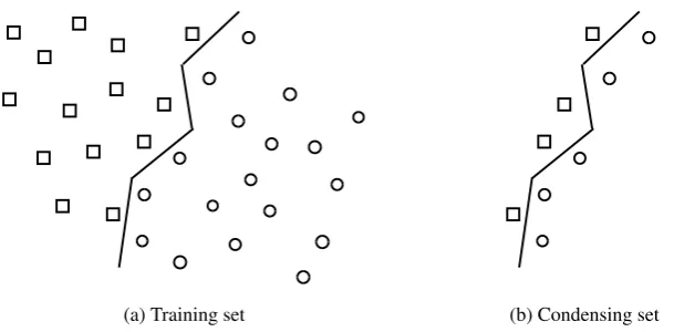
(a) Training set (b) Condensing set
Fig. 1.Initial training data and close-class-border data
In this paper, we attempt to improve the performance of IB2 by considering the idea of prototype abstraction. Our contribution is the development and evaluation of a prototype abstraction version of IB2 that we call Abstraction IB2 (AIB2). The proposed prototype abstraction algorithm retains all the properties of IB2, but it is faster and achieves higher reduction rates and improved accuracy.
CNN-rule and IB2 are presented in Section 2. Section 3 describes in detail the pro-posed AIB2 algorithm. Section 4 presents an experimental study wherek-NN is applied on the original training sets and the corresponding condensed sets built by CNN, IB2 and AIB2 on nine datasets. The experimental study is complemented by the statistical compar-ison of the three DRTs through the Wilcoxon signed ranks test [14]. Section 5 concludes the paper.
2.
CNN-rule and IB2
The Condensing Nearest Neighbour (CNN) rule [22] is the earliest and also a reference condensing algorithm. CNN-rule (and many other DRTs) builds its condensing set based on the following simple idea. Items that lie in the “internal” data area of a class (i.e., far from class decision boundaries) are useless during the classification process. Thus, they can be removed without loss of accuracy. By adopting this idea, CNN-rule tries to place into the condensing set only the items that lie in the close-class-border data areas. These are the only essential items for the classification process. Figure 1 depicts this strategy. The idea is that thek-NN classifier will be able to have similar accuracy using either the training set (Figure 1(a)) or the condensing set (Figure 1(b)). However, a scan of the condensing set involves much lower computational cost than that of the training set.
CNN-rule tries to keep the close-class-border items as follows (see Algorithm 1). Initially, a random item from the training set (T S) is moved to the condensing set (CS) (line 2). Then, CNN-rule applies the single nearest neighbour rule and classifies the items ofT Sby scanning the items ofCS(line 6). If an item is misclassified, it is moved from
T StoCS(lines 7–11). The algorithm continues until there are no moves fromT StoCS
Algorithm 1CNN-rule Input:T S
Output:CS 1: CS←∅
2: pick a random item ofT Sand move it toCS 3: repeat
4: stop←T RU E 5: foreachx∈T Sdo
6: N N←Nearest Neighbour ofxinCS 7: ifN Nclass̸=xclassthen
8: CS←CS∪ {x} 9: T S←T S− {x} 10: stop←F ALSE 11: end if
12: end for
13: untilstop==T RU E{no move during a pass ofT S} 14: discardT S
15: return CS
correctly classified by the content ofCS. The remaining content ofT Sis discarded (line 14) to save space.
CNN-rule considers that misclassified items are probably close to decision boundaries and so they must be included in the condensing set. An advantage is that it is a non-parametric approach. It determines the number of the prototypes automatically, without user-defined parameters. A drawback is that the resulting condensing set depends on the order in which class labels of items enter the condensing set. Therefore, CNN-rule builds a different condensing set by examining the same training data in a different order.
Furthermore, CNN-rule cannot handle new training data, i.e., is non-incremental. The algorithm involves multiple passes over the data and it cannot use training data available at a later time to update its condensing set. To construct an updated condensing set, CNN-rule needs the complete training set (new and old data), thus, the training items that do not enter the original condensing set should be retained. In addition, CNN-rule requires that all training items are memory resident.
Although IB2 is based on CNN-rule, it is faster and incremental. Therefore, it can handle new training data or datasets that cannot fit into memory. Actually, IB2 is an one-pass version of CNN-rule (see Algorithm 2) and works as follows. When a new itemx
of the training set (T S) arrives (line 3), it is classified by the single nearest neighbour rule by scanning the contents of the current condensing set (CS) (line 4). Ifxis wrongly classified, it is placed inCS(lines 5-7). Then,xis discarded since it has been examined (line 8).
Algorithm 2IB2 Input:T S Output:CS
1: CS←∅
2: pick a random item ofT Sand move it toCS 3: foreachx∈T Sdo
4: N N←Nearest Neighbour ofxinCS 5: ifN Nclass̸=xclassthen
6: CS←CS∪ {x} 7: end if
8: T S←T S− {x} 9: end for
10: return CS
placed or not in the condensing set, and then, removed. Additionally, IB2 can handle new class labels. All these properties render IB2 an appropriate condensing algorithm for dynamic/streaming environments where new training data may be gradually available or for training databases that cannot fit into the device’s memory.
Although many DRTs have been proposed during the past decades, here, we present only CNN-rule and IB2 because they are ancestors of the proposed algorithm. There are many other condensing algorithms that either extend the CNN-rule or are based on the same idea, i.e., the removal of the non-close-border data. Some of the these algorithms are the Reduced Nearest Neighbour (RNN) rule [20], the Selective Nearest Neighbour (SNN) rule [29], the Modified CNN rule [15], the Generalized CNN rule [10], the Fast CNN algorithms [6, 7], Tomek’s CNN rule [31], the Patterns with Ordered Projection (POP) algorithm [2, 28], the recently proposed Template Reduction for k-NN (TRkNN) [16], the Prototype Selection by Clustering (PSC) algorithm [26, 27] and of course the IB2 algorithm [3, 4].
3.
The proposed AIB2 algorithm
The proposed Abstraction IB2 (AIB2) algorithm is a prototype abstraction version of IB2. Therefore, AIB2 is a non-parametric, fast, one-pass prototype abstraction algorithm. It is also appropriate for dynamic/streaming environments and can handle new class labels. Like IB2, it can be applied on very large datasets that cannot fit into main memory or on devices with limited main memory (e.g., sensor networks), without transferring data to a server over a network for processing. The latter is usually costly and time-consuming. Certainly, like IB2, AIB2 does not take into account the phenomenon of concept drift [33] that may exist in data streams. IBL-DS [8] is based on the idea of IBL family of algorithms that can effectively deal with this phenomenon.
Algorithm 3AIB2 Input:T S
Output:CS 1: CS←∅
2: pick a random itemyofT Sand move it toCS 3: yweight←1
4: foreachx∈T Sdo
5: N N←Nearest Neighbour ofxinCS 6: ifN Nclass̸=xclassthen
7: xweight←1
8: CS←CS∪ {x} 9: else
10: foreach attributeattr(i)do 11: N Nattr(i)←
N Nattr(i)×N Nweight+xattr(i)
N Nweight+1
12: end for
13: N Nweight←N Nweight+ 1
14: end if
15: T S←T S− {x} 16: end for
17: return CS
attribute that denotes the number of training items it represents. The weight values are used for updating the prototype attributes in the multidimensional space.
AIB2 is presented in Algorithm 3. Initially, the condensing set (CS) is populated by a random item of the training set (T S) whose weight is initialized to 1 (lines 2–3). For each itemxof T S, AIB2 searches inCSand retrieves its nearest prototypeN N (line 5). Ifxis misclassified, it is placed in CSand its weight is initialized to one (lines 6– 8). Ifxis correctly classified,N N’s attributes are updated by taking into consideration its current weight and the attributes of x. Effectively, N N “moves” towards xin the multidimensional space (lines 10–12). Finally, the weight ofN N is increased by 1 (line 13) andxis removed (line 15).
Figures 2 and 3 illustrate two-dimensional examples of AIB2 execution. Suppose that the current condensing set includes three prototypes, two of class circle and one of class square (Figure 2(a) and Figure 3(a)). Suppose that a new square item,a, arrives (Fig-ure 2(b)). AIB2 should decide whetherawill enter the condensing set or it will be used to update an existing prototype. Sinceais closer to a prototype of a different class,aenters the condensing set and its weight value is initialized to one (Figure 2(c)). In contrast, sup-pose that the new itemais a circle item (Figure 3(b)). Sinceais closer toP, which is a prototype of the same class,aupdatesP. ThereforePmoves towardsaand its weight is increased by one (Figure 3(c)). In our example, the updatedPlies in between the original
P andabecause the weight ofP was 1).
(a) Current condensing set (3 prototypes)
(b) New item arrival (c) The new item enters the condensing set
Fig. 2.AIB2 example: new prototype enters the condensing set
(a) Current condensing set (3 prototypes)
(b) New item arrival (c) Updating of nearest prototype
Fig. 3.AIB2 example: repositioning an existing prototype
is towards the new training item. Like IB2, AIB2 prototypes depend on the order of the training items. It is possible that over time and because of a non-uniform arrival of training data items, an AIB2 prototype will gradually move far away from some of the original training items that it represents. Still, AIB2 prototypes with large weights will move very slowly towards the new training data items. This is also a problem with IB2 that contrary to CNN-rule cannot guarantee correct classification of all examined training data.
The idea is that a condensing set built by AIB2 will contain better prototypes com-pared to the condensing set built by IB2 and will achieve higher classification accuracy. In addition, we expect that updating the prototypes will reduce the number of items that enter the condensing set (lines 6–8), and thus, AIB2 will achieve higher reduction rates and lower preprocessing cost compared to IB2.
4.
Performance Evaluation
4.1. Experimental setup
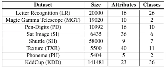
The three presented DRTs were evaluated using eight datasets distributed by the KEEL repository2[5] and summarized in Table 1. Seven datasets (all except KDD) were used
2
without applying data normalization. Datasets MGT, SI and TXR are distributed sorted on the class label. This affects all examined DRTs because their performance depends on the order of data in the training set. Therefore, we randomized the items of these datasets. The three algorithm implementations were written in C and Euclidean distance was the distance metric used.
Table 1.Datasets description
Dataset Size Attributes Classes
Letter Recognition (LR) 20000 16 26
Magic Gamma Telescope (MGT) 19020 10 2
Pen-Digits (PD) 10992 16 10
Sat Image (SI) 6435 36 6
Shuttle (SH) 58000 9 7
Texture (TXR) 5500 40 11
Phoneme (PH) 5404 5 2
KddCup (KDD) 141481 23 36
The KDD dataset includes 494,020 items and 41 attributes. However, huge amounts of data are duplicates and some attributes are unnecessary (three nominal and two fixed-value attributes). We removed all duplicates and the five unnecessary attributes. Conse-quently, the transformed KDD dataset includes 141,481 items and 36 attributes. It is worth mentioning that duplicates are useless especially fork-NN classification withk= 1. They do not influence the accuracy and negatively affect the computational cost. Although, for k > 1, duplicates may influence the accuracy, they should be removed, especially when fast execution of classification is required. In addition, the value ranges of the KDD dataset attributes vary extremely. Therefore, we normalized all attributes to the interval
[0,1]as follows. Assume that the dataset includesnitems and an attributeeshould be normalized to[0,1]. The normalized attribute value of thei-th item,i= 1, . . . , nis:
norm(ei) =
ei−Emin
Emax−Emin
whereEminandEmaxare the minimum and maximum values for attributee, respectively. Finally, we randomized the dataset.
We did not include more DRTs in our experimentation because our purpose was to focus on incremental and non-parametric DRTs. Of course, CNN-rule is non-incremental, but it is considered a reference DRT and is being used in many papers for comparison purposes. In addition, CNN-rule is the ancestor of IB2 and AIB2 and it makes sense to use it in our experiments.
sets distributed by the KEEL repository. For the transformed KDD dataset, we created the appropriate for cross-validation training/testing pairs. Of course, all measurements were estimated after the arrival of all training items.
The original form of the MGT dataset contains high levels of noise. Noisy items are misleading for the three DRTs and negatively affect reduction rates and the corresponding accuracies. Thus, we tried to build a noise-free version of the MGT dataset. To achieve this, we ran an editing algorithm before the execution of the DRTs. In particular, we coded in C the Edited Nearest Neighbour (ENN) rule [36], which is the reference editing algorithm. ENN-rule removes noisy items by using the following rule: a training item is removed if its class label does not agree with the majority of itsknearest neighbours in the initial training set. Consequently, ENN-rule needs to compute all distances among the training items, i.e., N∗(N2−1) distances, whereN is the number of the training items. By applying ENN-rule (withk = 3, see [19, 25, 35]) on each training portion of each fold, we built an extra dataset that we call MGT-ENN. Of course, the testing portions were not edited by the ENN-rule. We tested the three DRTs on both forms of the MGT dataset.
4.2. Comparisons
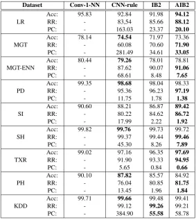
The results of our experimental study are presented in Table 2. Each column lists the results related to a classifier. Best measurements are in bold. The preprocessing cost mea-surements are in million distance computations. For reference, Table 2 presents the accu-racy measurements obtained by the conventional 1-NN classifier on the original training set under the label Conv-1-NN.
We should clarify that the reduction rates of MGT-ENN do not take into account the items removed by editing. They concern the size of the condensing set in relation to that of the edited set. Note that ENN-rule considered as noise 20.08% of MGT items on average. Therefore, the training portions of MGT-ENN include 20.08% fewer items than MGT on average.
Although the three DRTs did not reach the accuracy levels of Conv-1-NN, they were very close to them. With the exception of LR, SI and TXR, CNN-rule was more accurate than IB2 and AIB2. However, it required much higher preprocessing cost and it achieved lower reduction rates than IB2 and AIB2.
As we anticipated, the proposed algorithm performed better than IB2 in most datasets and in terms of all comparison criteria. KDD is the only dataset where IB2 seems to be better than AIB2. In the LR, SI and TXR datasets, AIB2 was more accurate than CNN-rule. Although we expected even better performance, we believe that the improvements achieved by AIB2 are noteworthy.
Moreover, as we expected, ENN-rule improved the efficiency of the classification pro-cess on MGT data. Accuracies and reduction rates achieved by the three DRTs on MGT-ENN (edited data) are higher than the corresponding measurements for MGT (non edited data).
4.3. Non-parametric statistical test
Table 2.DRTs Comparison in terms of Accuracy (Acc(%)), Reduction Rate (RR(%)) and Prepro-cessing Cost (PC(M))
Dataset Conv-1-NN CNN-rule IB2 AIB2
LR
Acc: 95.83 92.84 91.98 94.12
RR: - 83,54 85.66 88.12
PC: - 163.03 23.37 20.10
MGT
Acc: 78.14 74.54 71.97 73.36
RR: - 60.08 70.60 71.90
PC: - 281.49 34.61 33.05
MGT-ENN
Acc: 80.44 79.26 78.01 78.81
RR: - 87.62 90.07 91.06
PC: - 68.61 8.48 7.65
PD
Acc: 99.35 98.68 98.04 98.33
RR: - 95.36 96.23 97.19
PC: - 11.75 1.78 1.38
SI
Acc: 90.60 88.21 86.87 89.42
RR: - 80.22 84.62 86.72
PC: - 17.99 2.22 1.92
SH
Acc: 99.82 99.76 99.73 99.72
RR: - 99.37 99.44 99.46
PC: - 45.30 8.26 7.89
TXR
Acc: 99.02 97.16 96.35 97.69
RR: - 91.90 93.33 94.95
PC: - 5.65 0.84 0.66
PH
Acc: 90.10 87.82 85.57 84.92
RR: - 76.04 80.85 81.75
PC: - 13.45 1.96 1.84
KDD
Acc: 99.71 99.66 99.48 99.41
RR: - 99.12 99.26 99.21
PC: - 384.90 55.58 58.78
measurements of an extra criterion that estimates the overall classification performance of an algorithm. Our criterion adopts the idea presented in the statistical comparissons in [17, 18]. More specifically, the overall classification performance measurements were computed by averaging the normalized (to the range[0,1]) measurements of the three criteria. Note that since the higher the preprocessing cost, the lower the classification performance, we used1−normalized(P C)as the preprocessing cost. The overall clas-sification performance criterion combines the three criteria by considering all of them as having the same significance.
CNN-rule in terms of preprocessing cost. On the other hand, although it is clear that AIB2 is faster than IB2, this is not statistically supported (note that we have adopted the strict thresholdW ilc. = 0.05). Finally, we observe that AIB2 is statistically better than the other algorithms in terms of the overall classification performance.
Concerning CNN-rule and IB2 (last table row), we observe that IB2 is statistically better than rule in terms of reduction rate and preprocessing cost. In contrast, CNN-rule is statistically better than IB2 in terms of accuracy.
Table 3.Results of Wilcoxon signed ranks test
Methods ACC RR PC Overall performance
W/L Wilcoxon W/L Wilcoxon W/L Wilcoxon W/L Wilcoxon AIB2 vs CNN 3/6 0.767 9/0 0.008 9/0 0.008 9/0 0.008 AIB2 vs IB2 6/3 0.066 8/1 0.015 8/1 0.086 7/2 0.028 IB2 vs CNN 0/9 0.008 9/0 0.008 9/0 0.008 9/0 0.008
5.
Conclusions
Data reduction is an important research issue in the context ofk-NN classification. This paper proposed the AIB2 algorithm, an abstraction DRT that is based on the well-known condensing IB2 algorithm. The main concept behind AIB2 is that each generated pro-totype should be near to the center of the data area it represents. Like IB2 and contrary to CNN-rule and many other DRTs, AIB2 is an incremental DRT. This property renders AIB2 appropriate for dynamic domains where new training data is gradually available and for datasets that cannot fit into main memory.
The experimental results illustrate that AIB2 can achieve higher reduction rates and classification accuracy and lower preprocessing cost than IB2. In addition, AIB2 is prefer-able to CNN-rule when preprocessing cost and/or reduction rates are more critical criteria than accuracy and, of course, when an incremental DRT is required. The improvement offered by AIB2 was statistically confirmed by the Wilcoxon signed ranks test.
Acknowledgments.Stefanos Ougiaroglou is supported by a scholarship from the State Scholar-ships Foundation (I.K.Y.) of Greece.
References
1. Aggarwal, C.: Data Streams: Models and Algorithms. Advances in Database Systems Series, Springer Science+Business Media, LLC (2007)
2. Aguilar, J.S., Riquelme, J.C., Toro, M.: Data set editing by ordered projection. Intell. Data Anal. 5(5), 405–417 (Oct 2001), http://dl.acm.org/citation.cfm?id= 1294007.1294010
4. Aha, D.W., Kibler, D., Albert, M.K.: Instance-based learning algorithms. Mach. Learn. 6(1), 37–66 (Jan 1991),http://dx.doi.org/10.1023/A:1022689900470
5. Alcal´a-Fdez, J., Fern´andez, A., Luengo, J., Derrac, J., Garc´ıa, S.: Keel data-mining soft-ware tool: Data set repository, integration of algorithms and experimental analysis framework. Multiple-Valued Logic and Soft Computing 17(2-3), 255–287 (2011)
6. Angiulli, F.: Fast condensed nearest neighbor rule. In: Proceedings of the 22nd international conference on Machine learning. pp. 25–32. ICML ’05, ACM, New York, NY, USA (2005) 7. Angiulli, F.: Fast nearest neighbor condensation for large data sets classification. IEEE Trans.
on Knowl. and Data Eng. 19(11), 1450–1464 (Nov 2007), http://dx.doi.org/10. 1109/TKDE.2007.190645
8. Beringer, J., H¨ullermeier, E.: Efficient instance-based learning on data streams. Intell. Data Anal. 11(6), 627–650 (Dec 2007), http://dl.acm.org/citation.cfm?id= 1368018.1368022
9. Brighton, H., Mellish, C.: Advances in instance selection for instance-based learning algo-rithms. Data Min. Knowl. Discov. 6(2), 153–172 (Apr 2002),http://dx.doi.org/10. 1023/A:1014043630878
10. Chou, C.H., Kuo, B.H., Chang, F.: The generalized condensed nearest neighbor rule as a data reduction method. In: Proceedings of the 18th International Conference on Pattern Recognition - Volume 02. pp. 556–559. ICPR ’06, IEEE Computer Society, Washington, DC, USA (2006),
http://dx.doi.org/10.1109/ICPR.2006.1119
11. Cover, T., Hart, P.: Nearest neighbor pattern classification. IEEE Trans. Inf. Theor. 13(1), 21–27 (Sep 2006),http://dx.doi.org/10.1109/TIT.1967.1053964
12. Dasarathy, B.V.: Nearest neighbor (NN) norms : NN pattern classification techniques. IEEE Computer Society Press (1991)
13. Dasarathy, B.V., Snchez, J.S., Townsend, S.: Nearest neighbour editing and condensing toolssynergy exploitation. Pattern Analysis & Applications 3(1), 19–30 (2000),http://dx. doi.org/10.1007/s100440050003
14. Demˇsar, J.: Statistical comparisons of classifiers over multiple data sets. J. Mach. Learn. Res. 7, 1–30 (Dec 2006),http://dl.acm.org/citation.cfm?id=1248547.1248548
15. Devi, V.S., Murty, M.N.: An incremental prototype set building technique. Pattern Recognition 35(2), 505–513 (2002)
16. Fayed, H.A., Atiya, A.F.: A novel template reduction approach for the k-nearest neigh-bor method. Trans. Neur. Netw. 20(5), 890–896 (May 2009),http://dx.doi.org/10. 1109/TNN.2009.2018547
17. Garc´ıa, S., Cano, J.R., Herrera, F.: A memetic algorithm for evolutionary prototype selection: A scaling up approach. Pattern Recogn. 41(8), 2693–2709 (Aug 2008),http://dx.doi. org/10.1016/j.patcog.2008.02.006
18. Garcia, S., Derrac, J., Cano, J., Herrera, F.: Prototype selection for nearest neighbor classifica-tion: Taxonomy and empirical study. IEEE Trans. Pattern Anal. Mach. Intell. 34(3), 417–435 (Mar 2012),http://dx.doi.org/10.1109/TPAMI.2011.142
19. Garc´ıa-Borroto, M., Villuendas-Rey, Y., Carrasco-Ochoa, J.A., Mart´ınez-Trinidad, J.F.: Us-ing maximum similarity graphs to edit nearest neighbor classifiers. In: ProceedUs-ings of the 14th Iberoamerican Conference on Pattern Recognition: Progress in Pattern Recognition, Im-age Analysis, Computer Vision, and Applications. pp. 489–496. CIARP ’09, Springer-Verlag, Berlin, Heidelberg (2009),http://dx.doi.org/10.1007/978-3-642-10268-4_ 57
20. Gates, G.W.: The reduced nearest neighbor rule. ieee transactions on information theory. IEEE Transactions on Information Theory 18(3), 431–433 (1972)
22. Hart, P.E.: The condensed nearest neighbor rule. IEEE Transactions on Information Theory 14(3), 515–516 (1968)
23. Jankowski, N., Grochowski, M.: Comparison of instances seletion algorithms i. algorithms survey. In: Artificial Intelligence and Soft Computing - ICAISC 2004, LNCS, vol. 3070, pp. 598–603. Springer Berlin / Heidelberg (2004)
24. Lozano, M.: Data Reduction Techniques in Classification processes (Phd Thesis). Universitat Jaume I (2007)
25. Olvera-L´opez, J.A., Carrasco-Ochoa, J.A., Mart´ınez-Trinidad, J.F., Kittler, J.: A review of in-stance selection methods. Artif. Intell. Rev. 34(2), 133–143 (Aug 2010),http://dx.doi. org/10.1007/s10462-010-9165-y
26. Olvera-Lopez, J.A., Carrasco-Ochoa, J.A., Trinidad, J.F.M.: A new fast prototype selection method based on clustering. Pattern Anal. Appl. 13(2), 131–141 (2010)
27. Ougiaroglou, S., Evangelidis, G.: Fast and accurate k-nearest neighbor classification using pro-totype selection by clustering. In: 16th Panhellenic Conference on Informatics (PCI), 2012. pp. 168–173 (2012)
28. Riquelme, J.C., Aguilar-Ruiz, J.S., Toro, M.: Finding representative patterns with ordered pro-jections. Pattern Recognition 36(4), 1009 – 1018 (2003),http://www.sciencedirect. com/science/article/pii/S003132030200119X
29. Ritter, G., Woodruff, H., Lowry, S., Isenhour, T.: An algorithm for a selective nearest neighbor decision rule. IEEE Trans. on Inf. Theory 21(6), 665–669 (1975)
30. Samet, H.: Foundations of multidimensional and metric data structures. The Morgan Kaufmann series in computer graphics, Elsevier/Morgan Kaufmann (2006)
31. Tomek, I.: Two modifications of cnn. Systems, Man and Cybernetics, IEEE Transactions on SMC-6(11), 769–772 (Nov 1976)
32. Triguero, I., Derrac, J., Garcia, S., Herrera, F.: A taxonomy and experimental study on proto-type generation for nearest neighbor classification. Trans. Sys. Man Cyber Part C 42(1), 86–100 (Jan 2012),http://dx.doi.org/10.1109/TSMCC.2010.2103939
33. Tsymbal, A.: The problem of concept drift: definitions and related work. Tech. Rep. TCD-CS-2004-15, The University of Dublin, Trinity College, Department of Computer Science, Dublin, Ireland (2004)
34. Weber, R., Schek, H.J., Blott, S.: A quantitative analysis and performance study for similarity-search methods in high-dimensional spaces. In: Proceedings of the 24rd International Con-ference on Very Large Data Bases. pp. 194–205. VLDB ’98, Morgan Kaufmann Publish-ers Inc., San Francisco, CA, USA (1998),http://dl.acm.org/citation.cfm?id= 645924.671192
35. Wilson, D.R., Martinez, T.R.: Reduction techniques for instance-basedlearning algo-rithms. Mach. Learn. 38(3), 257–286 (Mar 2000), http://dx.doi.org/10.1023/A: 1007626913721
36. Wilson, D.L.: Asymptotic properties of nearest neighbor rules using edited data. IEEE trans. on systems, man, and cybernetics 2(3), 408–421 (July 1972)
instructor at ATEI of Messolonghi, Greece. His research interests include Data Mining, Mobile Computing, and Educational Technology.
Georgios Evangelidisis a Professor at the Department of Applied Informatics, Univer-sity of Macedonia, Greece. He has a B.Sc. in Mathematics (Aristotle UniverUniver-sity of Thes-saloniki, Greece, 1987) and a M.Sc. and Ph.D. in Computer Science (Northeastern Uni-versity, Boston, MA, USA, 1990 and 1994, respectively). His interests include database technologies, data mining, citation analysis and software engineering. He has participated in various EU funded projects and has published over 100 scientific papers in refereed journals and conferences. He is a member of the DBTechNet initiative.