[NORMAL] An optimization model for aggregate production planning and control: a genetic algorithm approach

An Optimization Model for Aggregate Production Planning and

Control: A Genetic Algorithm Approach

S. A. Ahmed, T. K. Biswas, C. K. Nundy

Department of Industrial and Production Engineering, Jashore University of Science and Technology, Jahsore, Bangladesh.

A B S T R A C T

In this paper, an optimization model for aggregate planning of multi-product and multi-period production system has been formulated. Due to the involvement of too many stakeholders as well as uncertainties, the aggregate production planning sometimes becomes extremely complex in dealing with all relevant cost criteria. Most of the existing approaches have focused on minimizing only production related costs, consequently ignored other cost factors, for instance, supply chain related costs. However, these types of other cost factors are greatly affected by aggregate production planning and its mismanagement often results in increased overall costs of the business enterprises. Therefore, the proposed model has attempted to incorporate all the relevant cost factors into the optimization model which are directly or indirectly affected by the aggregate production planning. In addition, the considered supply chain related costs have been segregated into two major categories. While the raw material purchasing, ordering, and inventory costs have been grouped into an upstream category, finished goods inventory, and delivery costs in the downstream category. The most notable differences with the other existing models of aggregate production planning are in the consideration of the cost factors and formulation process in the mathematical model. A real-life industrial case problem is formulated and solved by using a genetic algorithm to demonstrate the applicability and feasibility of the proposed model. The results indicate that the proposed model is capable of solving any type of aggregate production planning efficiently and effectively.

Keywords: Aggregate production planning, Cost optimization, Genetic algorithm, Production system.

Article history: Received: 06 May 2019 Revised: 23 July 2019 Accepted: 07 September 2019

1. Introduction

Aggregate Production Planning (APP) refers to 3 to 18 months of medium-term capacity planning. The main objective of this planning is to meet fluctuating demand over the planning horizon and to achieve customer satisfaction [1]. It mainly includes taking decision on production quantity, inventory, and workforce for the time horizon to ensure low cost product and timely

_{Corresponding author}

E-mail address:[email protected] DOI:10.22105/riej.2019.192936.1090

International Journal of Research in Industrial

delivery [2]. Al-e et al. [3] described APP as a method that aggregates all data related to manufacturing and determines the best way to fulfill expected requirements through the use of available physical resources. Dakka et al. [4] described the APP as a production approach predicting the existence of an aggregate production unit, such as volume, production time, or dollar value. In this dynamic business environment, the effective aggregate planning is seen as key to success of a manufacturing company. During the last three decades, both academic institutes and industries have put great effort into designing and developing effective approaches and methods for APP. One of the major objectives of these efforts were to develop cost optimization model for APP. Different types of algorithms have been used to develop these models. However, the manufacturing environment and cost parameters have been changed over time because of changes in customer requirements and technology improvements.

In this modern manufacturing scenario, matching of supply and demand has become a major challenge to thrive for the manufacturing companies [5]. However, the proper APP helps matching supply and demand while reducing total costs. The aggregate plan output consists of the total quantities of each product or product group to be manufactured during the scheduling period of the various manufacturing activities required to achieve the planned levels of production. It intends to set general manufacturing objectives and to help plan the accessibility of additional inputs and support operations to fulfill manufacturing objectives. There are various types of mathematical techniques and models to perform the task of APP.

Many researchers have developed integrated approach to address the aggregate production problems and presented many models integrating different algorithms and techniques to solve the problems [6-9]. Although, main objective of all these models was to minimize overall production costs, they also focused on other important decision variables. However, production cost structure and manufacturing environment have become very dynamic. As a result, models for solving aggregate production problem also require the consideration of these factors. Again, there exists variety in type of production and also in production time. Traditional models lack the considerations of these important factors in solving APP problems.

The rest of this paper is organized as follows. Section 2 describes the previous literatures on aggregate production planning. Section 2 describes the problem, details assumptions, and develops the aggregate production planning cost optimization model. Section 3 outlines the step by step procedure of GA. Section 4 presents a numerical example to demonstrate the application of proposed cost optimization model for an electronic company. Section 5 discusses the findings from the application of the model. The final section draws conclusions and make relevant recommendations.

2. Literature Review

Although the issue of APP was introduced in the 1950s, it is still extensively researched by many researchers. Over the past few decades, they have constructed various models, each with their own pros and cons, to effectively solve the aggregate production planning problem. They also classified each method as being capable of either generating an optimal or near-optimal solution.

Some researchers used linear programming approaches with different application cases to solve APP problem. Hsieh and Wu [10] created a deterministic linear programming model for APP with an imprecise nature. This research examines how the imprecise nature of the Computer-Integrated Production Management System (CIPMS) affects the outcomes of the planning. Wang and Fang [11] suggested Fuzzy Linear Programming (FLP) technique for solving the issue of APP with different objectives where the item price, the unit cost to subcontract, the workforce level, the manufacturing capability, and the market requirements are inherently fuzzy. However, the limitation of this model is that it applied the conventional mathematical programming technique to medium-term production planning. Wang and Liang [12] proposed an interactive multiple fuzzy objective linear programming model for solving the aggregate production decision problem in fuzzy environment. They considered the time value of money to construct constraints of this model. Gulsun et al. [13] outlined the LP model for aggregate production planning to determine the most appropriate approach while minimizing general production costs and minimizing the impact of hiring or layoff decisions on the level of motivation of the workers. An integrated model combining with linear programming, simulation, and interactive approach was proposed by Nowak [14] in which the linear programming models were used to generate initial solutions, simulation experiments were performed to check the fluctuation in demands and interactive procedure was used for identifying the final solution of the problem. Chakrabortty et al. [15] developed multi-period and multi-product APP which was formulated as an integer linear programming model using a triangular possibility distribution [15].

In this study, authors have used a popular meta-heuristic, GA to solve the proposed aggregate product model. GA is a nature inspired algorithm which has become very popular in solving aggregate production problem. The early evolution of GA can be observed from late 1950’s and early-1960’s [19]. Ramezanian et al. [20] used Mixed Integer Linear Programming (MILP) to formulate two-phase aggregate production planning problem and applied GA combined with tabu search to solve the problem. However, cost parameters were not explicitly considered in this case. Chakrabortty and Hasin [21] carried out a case study on a readymade garments in Bangladesh. They suggested an APP model with an adaptive Fuzzy-Based Genetic Algorithm (FBGA) technique to solve a two-product and two-period APP with some susceptible management constraints such as imprecise requirements, varying production expenses, etc. Hossain et al. [22] developed a mathematical model for solving APP using GA and big M method. Savsani et al. [23] applied GA to develop aggregate production planning model. However, this model lacks consideration of explicit cost structure in the optimization model. Mahmud et al. [24] developed an APP model in possibilistic environment applying multi-objective GA. Apart from these, many other mathematical models of aggregate production planning problem have been developed applying different meta-heuristic algorithms [25-27]. However, most of these works lack the consideration of explicit cost structures in their models. Therefore, current research aims to develop an optimization model for aggregate production planning considering explicit cost structures. To achieve this objective, GA has been applied.

3. Problem Formulation

3.1. Problem Assumptions

The aggregate production problem for multi-product and multi-period can be described as follows. Assume that a company manufactures 𝑛 types of products over a planning horizon 𝑡 to satisfy market demand. This model aims to build a single objective GA to determine the optimum aggregate strategy for meeting specified demand by changing periodic and overtime manufacturing rates, inventory levels, labor levels, subcontracting and back-ordering rates, order amount, waste level, and other controllable variables. The mathematical model herein is created on the basis of the above characteristics on the following assumptions.

 All parameter values are fixed over the next t planning horizon.

 The intensifying variables are resolved over the next 𝑡 planning horizon in each of the cost categories.

 Current levels of labor, machine capacity, inventory, backorder, order quantity per period and warehouse space cannot exceed their respective peak levels in each period.

 The fixed demand over a given period can either be satisfied or backordered, but in the next period, the backorder must be met.

 For the development of the model, some confidential information that is not provided to others from the sector has been assumed.

 Workers are trained in every period of time to obtain the necessary level of expertise.  Work In Process (WIP) inventory cost is not considered.

 The specified time horizon contains two monthly periods.  Each type of products is assigned to just one production line.

In this research, authors have considered maximum types of costs and formulated the APP model and try to solve the APP model with GA.

3.2. Problem Notation

n −- Specific product types.

t − No. of periods.

Dt− Demand uncertain for nth product in period (𝑡) (units) (Forecasted).

𝑅𝑥𝑡− Regular time production of 𝑛th Product in period 𝑡 (units).

𝑅𝑐𝑡− Regular time production cost per unit for 𝑛th product in period 𝑡 (TK/unit).

𝑖𝑟− Escalating factors regular time production cost (%).

𝑂𝑥𝑡− Overtime production of 𝑛th product in period 𝑡 (units).

𝑂𝑐𝑡− Overtime production cost per unit of 𝑛th product in period 𝑡 (TK/unit).

𝑖𝑜− Escalating factors overtime production cost (%).

𝑆𝑥𝑡− Subcontracting production of 𝑛th product in period 𝑡 (units).

𝑆𝑐𝑡− Subcontracting production cost per unit for 𝑛th product in period 𝑡 (TK/unit).

𝑖𝑠− Escalating factors subcontracting production cost (%).

𝐼𝑓𝑛𝑡− Inventory level of finished goods in 𝑛th product in period 𝑡 (unit)

𝐼𝑓𝑐𝑡− Inventory carrying cost of finished goods per unit for 𝑛th product in period 𝑡 (TK/unit).

𝐼𝑟𝑛𝑡− Inventory level of raw material per unit 𝑛th product in period 𝑡 (unit).

𝐼𝑟𝑐𝑡− Inventory carrying cost of raw material per unit for 𝑛th product in period 𝑡 (TK/unit).

𝑖𝑓𝑟− Escalating factors inventory carrying cost (%).

𝐵𝑛𝑡− Back order of 𝑛th product in period 𝑡 (unit).

𝐵𝑐𝑡− Back order cost per unit for 𝑛th product in period 𝑡.

𝑖𝑏− Escalating factors for back order cost.

𝐻𝑛𝑡− Hired worker in period 𝑡 (man hour).

𝐻𝑐𝑡− Cost of hired in period 𝑡 (TK/man hour).

𝐹𝑛𝑡− Worker fired in period 𝑡 (man hour).

𝐹𝑐𝑡− Cost of fired worker in period 𝑡 (TK/man hour).

𝑖𝑓− Escalating factor to hire and fire cost (%).

𝑇𝑅𝑛𝑡− No. of training workers.

𝑇𝑅𝑐𝑡− Average cost for training per unit labor (TK/unit).

𝑖𝑡− Escalating factors of training cost (%).

𝑊𝑥𝑛𝑡− Wastage level of 𝑛th product in period 𝑡 (unit).

𝑊𝑐𝑡− Wastage cost per unit in 𝑛th product in period 𝑡.

𝐴𝑊𝑛𝑡− Allowable wastage produce in factory (unit).

𝑊𝑃𝑛𝑡− Average percentage of wastage of 𝑛th product in period 𝑡 (unit).

𝑂𝑑𝑐𝑡− Average ordering cost per order for 𝑛th product in period 𝑡.

𝑂𝑑𝑛𝑡- No. of order for nth product in period 𝑡.

𝑖𝑜𝑟− Escalating factors of ordering cost (%).

𝐿𝑛𝑡− Hours of labor usage per unit of 𝑛th product in period 𝑡 (Machine-hour/unit).

𝐻𝑜𝑛𝑡−Hours of machine usage per unit of 𝑛th product in period 𝑡 (machine-hour/unit).

𝐿𝑚𝑎𝑥− Maximum labor level available in period 𝑡 (man hour).

𝑀𝐶𝑡𝑚𝑎𝑥− Maximum machine capacity available in period 𝑡 (machine-hour).

𝑊𝐻𝑡𝑚𝑎𝑥− Maximum warehouse spaces available in period 𝑡 (feet).

𝑚𝑖𝑛𝑖𝑓− Minimum quantity of finished goods inventory per product.

𝑚𝑖𝑛𝑖𝑟− Minimum quantity of raw material inventory per product.

𝑚𝑎𝑥𝑖𝑓− Maximum quantity of finished goods inventory per product.

𝑚𝑎𝑥𝑖𝑟− Maximum quantity of raw material inventory per product.

𝑚𝑎𝑥𝑤- Maximum number of workers for product in period 𝑡.

𝐵𝑛𝑡𝑚𝑎𝑥- Maximum number of unit backordered nth product in period t.

𝑇𝑤𝑛𝑡− Total number of workers in the industry (average).

𝐵𝑛(𝑡−1)− Number of unit backordered 𝑛th product in period 𝑡 − 1 (Units).

𝐼𝑟𝑛(𝑡−1)− Number of units held in raw material inventory 𝑛th product in period 𝑡 − 1 (Units).

𝐼𝑓𝑛(𝑡−1)− Number of units held in finished goods inventory 𝑛th product in period 𝑡 − 1 (Units).

3.3. Decisions Variables

𝑅𝑥𝑛𝑡− Regular time production in 𝑛th product in period 𝑡 (Units).

𝑂𝑥𝑛𝑡− Over time production in 𝑛th product in period 𝑡 (Units).

𝑆𝑥𝑛𝑡− Subcontracting volume of 𝑛th product in period 𝑡 (Units).

𝐵𝑛𝑡− Number of backordered for 𝑛th product in period 𝑡 (Units).

𝐼𝑟𝑛𝑡− Number of units held in raw material inventory 𝑛th product in period 𝑡 (Units).

𝐼𝑓𝑛𝑡− Number of units held in finished goods inventory 𝑛th Product in period 𝑡 (Units)

𝑊𝑥𝑛𝑡− Waste level of nth product in period 𝑡 (Units).

𝐻𝑛𝑡− Worker hired 𝑛th product in period 𝑡 (Man hour).

𝐹𝑛𝑡− Worker fired 𝑛th product in period 𝑡 (Man hour).

𝑂𝑑𝑛𝑡− Order quantity per order for 𝑛th product in period 𝑡 (units).

𝑇𝑟𝑛𝑡− Workers training for 𝑛th product in period 𝑡 (Man hour).

3.4. Single Objective APP Model

Mainly, the aim of owner of the industry is profit maximization or cost minimization to survive in the competitive market. For this reason, the authors have developed single objective cost minimization model for an electronic industry through summation of five types of different costs. Authors have also considered escalating factor for all type of cost as money value may change with time.

 Minimization of production costs:

Z1=∑nn=1 ∑tt=1 RxtRct(1 + ir)t+ BxtBct(1 + ib)t+ SxtSct(1 + is)t+OxtOct(1 + io)t. (1)

 Minimization of inventory costs:

Z2 =∑n=1n ∑t=1t (IrntIrct+ IfntIfct)(1 + ifr)t. (2)

 Minimization of ordering costs:

Z3=∑n=1n ∑tt=1 (Odct∗ (( Dt+ (Dt∗ WPnt))/Qnt)(1 + ior)t. (3)

𝑍4=∑n=1n ∑t=1t TrntTrct(1 + it)t. (4)

 Minimization of worker hiring and firing costs:

Z4=∑n=1n ∑tt=1 (HtHct+ FtFct)(1 + it)t. (5)

Now, combined with upper all objectives:

Zmin= ∑nn=1 ∑tt=1 (RxntRct(1 + ir)t+ BxntBct(1 + ib)t+ SxntSct(1 + is)t+OxntOct(1 +

io)t) +

∑n=1n ∑t=1t (IrntIrct+ IfntIfct)(1 + ifr)t+ ∑n=1n ∑tt=1 ((HntHct+ FntFct)(1 + ihf)t+

∑n=1n ∑tt=1 (WxtWct) (1 + iwi)t + ∑n=1n ∑ (Odct∗ (

Dt+ (Dt∗WPnt)

Qnt ) (1 + io)

t₊

t t=1

∑nn=1∑tt=1 TrntTrct(1 + it)t.

(6)

3.5. Constraints

3.5.1. Constraints on finished goods inventory

Certain demand for nth product in period (t) is equal to summation of regular time production in nth product in period and over time production in nth product in period t and subcontracting volume of nth product in period t and number of units backordered nth product in period t and number of units held in inventory nth product in period (t-1) and minus the summation of number of units held in inventory nth product in period t and number of units backordered nth product in period t-1.

𝐼𝑓𝑛𝑡 ≥ 𝑚𝑖𝑛𝑖 for∀n, ∀t. (8)

Number of units held in inventory nth product in period t is greater than minimum quantity of inventory per product of product t.

Ifnt≤ maxif for∀n, ∀t. (9)

Number of units held in finished goods inventory nth product in period t is less than maximum quantity of finished goods inventory per product of product t.

3.5.2. Constraints on raw material inventory

Irn(t−1)- Irnt+ Rnt+ Ont+ Snt= Dt+(Dt∗ WPnt) for ∀n, ∀t. (10)

Total demand with considering average percentage of wastage is equal to the summation of raw material inventory in period t-1 with other production unit and subtract the raw material inventory in period t.

Ifnt≤ maxir for ∀n, ∀t. (11)

Number of units held in raw material inventory nth product in period t is less than maximum quantity of raw material inventory per product of product t.

Ifnt≥ mini for ∀n, ∀t. (12)

Number of units held in raw material inventory nth product in period t is greater than minimum quantity of raw material inventory per product of product t.

3.5.3. Constraints on quantity per order, backordered, and subcontracting volume

Ont+Snt ≤Rnt for ∀n, ∀t. (13)

Regular time production for nth product in period t is greater than the summation of overtime production in nth product in period t and subcontracting volume of nth product in period t.

Bnt≤ Bntmax for ∀n, ∀t. (14)

Number of unit backordered nth product in period t is less than maximum number of unit backordered nth product in period t.

Qnt≥ 500 for ∀n, ∀t. (15)

Quantity per order for nth product in period t is always greater than 500.

3.5.4. Constraints on machine capacity and warehouse space

WHfnt∗Ifnt≤WHftmax for ∀n, ∀t. (16)

Maximum warehouse spaces available in period t is greater than the multiplication of warehouse spaces per unit of nth product in period t (feet) and number of units held in finish good inventory nth product in period t.

WHrnt∗Irnt≤ WHrtmax for ∀n, ∀t. (17)

Maximum warehouse spaces available in period t is greater than the multiplication of warehouse spaces per unit of nth product in period t (feet) and number of units held in raw material inventory nth product in period t

(Rxnt+Oxnt) ∗Hont ≤MCtmax for ∀n, ∀t. (18)

3.5.5. Constraints on labor levels

∑ ∑t

t=1 Ln(t−1)∗ ( n

n=1 Rn(t−1)+ On(t−1)) + Ht− Ft = ∑n=1n ∑t=1t Ln(t−1)∗ (Rnt+ Ont) for ∀n,

∀t. (19)

Here the equation represents a set of constraints in which the labor levels are identified by man hour in period t equal the labor levels in period t-1 plus new hires and subtraction of fires in period t.

∑ ∑t

t=1 Ln(t−1)∗ ( n

n=1 Rnt+ Ont) ≤ Lmax for ∀n, ∀t. (20)

Actual labor levels cannot exceed the maximum available labor levels in each period.

3.5.6. Constraints on wastage unit

(Rnt+Ont)* WPnt≤AWnt for ∀n, ∀t. (21)

Total value of the summation of regular time production in nth product in period and overtime

production in nth product in period t with multiplication of the percentage of wastage of nth

product in period t (unit) is less than waste level of nth product in period t.

3.5.7. Constraint on training labor

TRnt=∑n=1n Hnt for ∀n. (22)

Number of workers training for nth product in period t is equal to summation of the workers hired

for nth product for the same period t.

3.5.8. Constraint on non-negativity variables

Odnt- Hnt−Fnt− Ifnt− Irnt− Bnt− Rxnt- Oxnt- Sxnt− Wxnt- Trnt≥ 0 for ∀n, ∀t. (23)

The value of all decision variable must be greater than zero.

4. A Brief Outline of GA

Step 1. Generate a random population of chromosome, which is the right solution to the problem.

Step 2. Assess the fitness of the population of each chromosome (Fitness).

Step 3. Create a new population by repeating following steps until the new population is completed.

 Selection: Select two parent chromosomes from a population according to their fitness. Better fitness and bigger chance to be selected to be the parent.

 Crossover: With a crossover probability, cross over the parents to form new offspring, that is, children. If no crossover was performed, offspring is the exact copy of parents.  Mutation: With a mutation probability, mutate new offspring at each locus.

 Accepting: Place new offspring in the new population.

Step 4. Use new generated population for a further run of the algorithm.

Step 5. If the end condition is satisfied, stop, and return the best solution in current population.

Step 6. Go to Step 2.

Some associated terms of GA have been discussed below [29].

4.1. Crossover Options

Crossover options specify how the GA combines two individuals, or parents, to form a crossover child for the next generation. Here we have chosen five different crossover (scattered crossover, single point crossover, two point crossover, arithmetic crossover, and constraint-dependent crossover) options for five scenarios.

Scattered crossover: It creates a random binary vector and selects the genes where the vector is a 1 from the first parent, and the genes where the vector is a 0 from the second parent, and combines the genes to form the child. For example, if p1 and p2 are the parents such as p1 = [a b c d e f g h] and p2 = [1 2 3 4 5 6 7 8] and the binary vector is [1 1 0 0 1 0 0 0], then the function returns the following child 1 = [a b 3 4 e 6 7 8].

Single point crossover:It chooses a random integer n between 1 and number of variables and then selects vector entries numbered less than or equal to n from the first parent and selects vector entries numbered greater than n from the second parent. For example, if p1 and p2 are the parents such as p1 = [a b c d e f g h] and p2 = [1 2 3 4 5 6 7 8] and the crossover point is 3, the function returns the following child = [a b c 4 5 6 7 8].

entries numbered from m+1 ton, inclusive, from the second parent, vector entries numbered greater than n from the first parent. The algorithm then concatenates these genes to form a single gene. For example, if p1 and p2 are the parents such as p1 = [a b c d e f g h] and p2 = [1 2 3 4 5 6 7 8] and the crossover points are 3 and 6, the function returns the following child = [a b c 4 5 6 g h].

Arithmetic crossover: Itis a crossover operator that linearly combines two parent chromosome vectors to produce two new offspring according to the following equations:





Offspring1 a * Parent1 1 a * Parent2  





Offspring2 1 – a * Parent1 a * Parent2  

Where ‘a’ is a random weighting factor (chosen before each crossover operation).

4.2. Mutation Options

Mutation options specify how the GA makes small random changes in the individuals in the population to create mutation children. Mutation provides genetic diversity and enables the GA to search a broader space. Here the authors use constraint dependent mutation and adapt feasible mutation options. Adaptive feasible randomly generates directions that are adaptive with respect to the last successful or unsuccessful generation. The feasible region is bounded by the constraints and inequality constraints. A step length is chosen along each direction so that linear constraints and bounds are satisfied.

4.3. Creation Function

Creation function creates the initial population for GA. Here the authors choose feasible population & Constraint dependent options. Feasible population creates a random initial population that satisfies all bounds and linear constraints. It is biased to create individuals that are on the boundaries of the constraints and create well-dispersed populations. This is the default if there are linear constraints.

4.4. Selection Options

Selection options specify how the GA chooses parents for the next generation. Here the authors used only Tournament selection option for tournament size 2 and 4. Tournament selection chooses each parent by choosing Tournament size players at random and then choosing the best individual out of that set to be a parent.

4.5. Migration Options

individuals from one subpopulation replace the worst individuals in another subpopulation. Individuals that migrate from one subpopulation to another are copied. They are not removed from the source subpopulation.

The GAs performance is largely influenced by crossover and mutation operators. The block diagram representation of GA is shown in Figure 1.

4.6. Genetic algorithm parameters

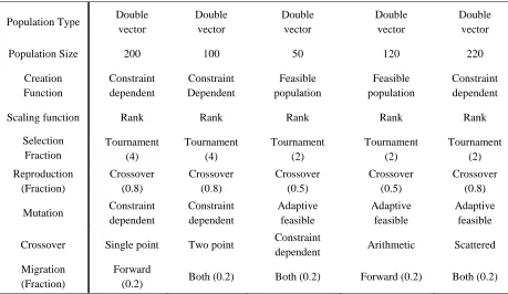
The authors have used MATLAB (2015a) computer software to solve the proposed Single Objective Genetic Algorithm (SOGA) approach for this case study. Total five runs were implemented considering five scenarios with different SOGA parameters shown in Table 1. Also Table 5 lists the single objective values for five SOGA runs through MATLAB.

Table 1. Different genetic algorithm options used for five scenarios.

Parameter Scenario 1 Scenario 2 Scenario 3 Scenario 4 Scenario 5

Population Type Double vector Double vector Double vector Double vector Double vector

Population Size 200 100 50 120 220

Creation Function Constraint dependent Constraint Dependent Feasible population Feasible population Constraint dependent

Scaling function Rank Rank Rank Rank Rank

Selection Fraction (size) Tournament (4) Tournament (4) Tournament (2) Tournament (2) Tournament (2) Reproduction (Fraction) Crossover (0.8) Crossover (0.8) Crossover (0.5) Crossover (0.5) Crossover (0.8)

Mutation Constraint

dependent Constraint dependent Adaptive feasible Adaptive feasible Adaptive feasible

Crossover Single point Two point Constraint

dependent Arithmetic Scattered

Migration (Fraction)

Forward

(0.2) Both (0.2) Both (0.2) Forward (0.2) Both (0.2)

5. Model Implementation

A well-known electronic industry was used as a case study to demonstrate the practicality of the proposed methodology. This company readily produces various electronic items and among them some are novel and some are expensive. Therefore, it requires a lot of appropriate observations and accurate manufacturing practices to gain the market and satisfy the buyers within specified lead time. Among various types of products, authors have collected data only for fan production sector and formulated aggregate production plan for table fan (Product 1) and another type of ceiling fan (Product 2).

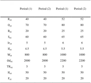
Table 2. List of relevant cost for all decision variables.

It is needed to know cost of the different product per unit for different period for solving APP problem as this is the cost minimization problem.

Items

Costs of Product-1 (TK)

Period (1) Period (2) Period (1) Period (2)

Rct 40 40 52 52

Oct 70 70 80 80

Bct 20 20 25 25

Sct 60 60 65 65

Irct 5 5 6 6

Ifct 4.5 4.5 5.5 5.5

Wct 800 800 1000 1000

Odct 2000 2000 2200 2200

TRct 5 5 5 5

Hct 50 50 50 50

Fct 20 20 20 20

Table 3. Initial data for two products.

𝐼𝑓𝑛(𝑡−1) (units) 2500 2800

𝐼𝑟𝑛(𝑡−1) (units) 3000 3200

𝑅𝑛(𝑡−1) 4800 5500

𝑂𝑛(𝑡−1) 950 1375

Total workers (people) 20 25

Regular + overtime working hour 10 10

No. of machine (units) 18 22

Total working day per period 25 25

Table 4. Other relevant data for calculation.

Items Period (1) Product-1 Period (2) Period (1) Product-2 Period (2)

Dt 6500 units 6200 units 7000 units 7200 units

maxif 3500 units 3500 4000 units 4000

maxir 3200 units 3200 3500 units 3500

minif 500 units 500 500 500

minir 500 units 500 500 units 500

Bntmax 350 units 350 300 300

WHftmax 3150 feet 3150 3200 feet 3200

WHfnt 0.9 feet - 0.8 feet -

WHrtmax 3840 3840 3500 3500

WHrnt 1.2 1.2 1.0 1.0

MCtmax 3600 m/c hour - 6875 m/c hour -

Hont 0.63 0.63 0.8 0.8

WPnt .025 .025 .030 .030

AWxt 200 units 200 units 250 units 250 units

Ln(t−1) 1.15 1.15 1.10 1.10

Lmax 7000 Man-hour 7000 7500 Man-hour 7500

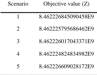
By putting above combination (from Table 1) in MATLAB software for optimization using with GA, the authors have got five different objective values for five different scenarios which are shown in Table 5.

Table 5. Calculated single-objective values for different scenario.

Scenario Objective value (Z)

1 8.462226845090458E9

2 8.462225795686462E9

3 8.462226017043371E9

4 8.462224824834982E9

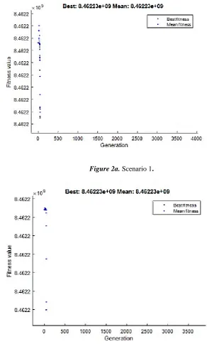
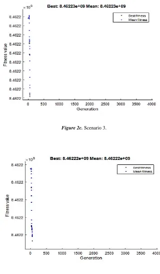
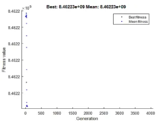
The authors have got graph comparing with fitness value to generation from GA tool from MATLAB for five different GA scenario. These 5 scenarios have been shown in Figure 2.

Figure 2a. Scenario 1.

Figure 2c. Scenario 3.

Figure 2e. Scenario 2.

Figure 2. Graph for five different scenario (a), (b), (c), (d) and (e) (source: MATLAB-2015a).

6. Results and Discussion

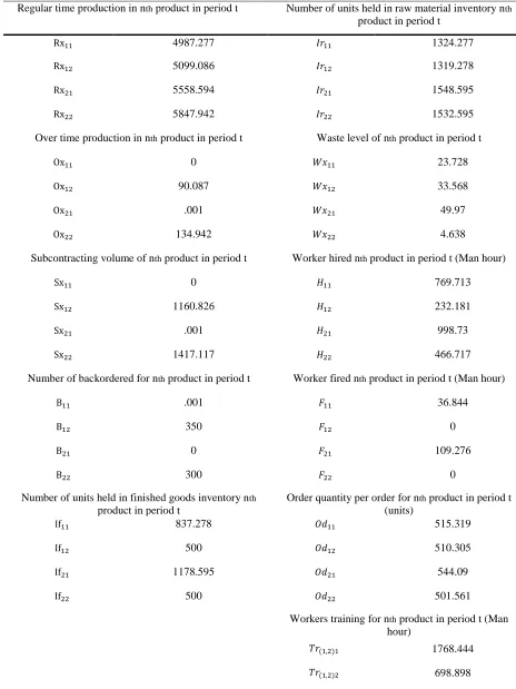
Table 6. Outputs of multi-product & multi-period APP plan for the case study (scenario 4).

Variables Optimized value Variables Optimized value

Regular time production in nth product in period t Number of units held in raw material inventory nth product in period t

Rx11 4987.277 𝐼𝑟11 1324.277

Rx12 5099.086 𝐼𝑟12 1319.278

Rx21 5558.594 𝐼𝑟21 1548.595

Rx22 5847.942 𝐼𝑟22 1532.595

Over time production in nth product in period t Waste level of nth product in period t

Ox11 0 𝑊𝑥11 23.728

Ox12 90.087 𝑊𝑥12 33.568

Ox21 .001 𝑊𝑥21 49.97

Ox22 134.942 𝑊𝑥22 4.638

Subcontracting volume of nth product in period t Worker hired nth product in period t (Man hour)

Sx11 0 𝐻11 769.713

Sx12 1160.826 𝐻12 232.181

Sx21 .001 𝐻21 998.73

Sx22 1417.117 𝐻22 466.717

Number of backordered for nth product in period t Worker fired nth product in period t (Man hour)

B11 .001 𝐹11 36.844

B12 350 𝐹12 0

B21 0 𝐹21 109.276

B22 300 𝐹22 0

Number of units held in finished goods inventory nth product in period t

Order quantity per order for nth product in period t (units)

If11 837.278 𝑂𝑑11 515.319

If12 500 𝑂𝑑12 510.305

If21 1178.595 𝑂𝑑21 544.09

If22 500 𝑂𝑑22 501.561

Workers training for nth product in period t (Man hour)

𝑇𝑟(1,2)1 1768.444

Note that, all the input variables of the proposed APP model are involved with substantial uncertainties, consideration of deterministic values may lead to poor performance of the model. Also, anticipations of the values of these variables with large quantity of historical datasets can improve the solution quality.

7. Conclusions

Over the last few decades, researchers have formulated many aggregate planning models considering various decision variables and using different solution technique. Most of them have primarily focused on minimizing production related costs, and ignored others type of costs like supply chain related costs. However, many supply chain related costs, both upstream and downstream are directly or indirectly affected by aggregate production planning. In this research, authors addressed this gap along with other production related costs which have often been overlooked in past studies such as training costs, hiring costs, and wastage costs. The novelty of this work lies on the formulation of the mathematical model and consideration of the cost factors. The results of the case study indicated that the proposed model can be effectively applied in real-life multi-product multi-period aggregate production planning. Although the proposed model is applied in electronic factory, it is quite general and expected to be applied in any other types of factory with minor modifications. This provides decision support to managers in setting up APP in order to achieve maximum profit by minimizing the total costs. The developed APP model has been solved by using GA, however other meta-heuristic optimization techniques including Particle Swarm Optimization (PSO), Simulated Annealing, Ant Colony Optimization and Artificial Bee Colony Optimization can also be employed [30-32]. Designing an APP model considering uncertain cost factors for large size problem can be a potential future research direction.

References

Gansterer, M. (2015). Aggregate planning and forecasting in make-to-order production systems.

International journal of production economics, 170, 521-528.

Kumar, G. M., & Haq, A. N. (2005). Hybrid genetic—ant colony algorithms for solving aggregate production plan. Journal of advanced manufacturing systems, 4(01), 103-111.

Al-e, S. M. J. M., Aryanezhad, M. B., & Sadjadi, S. J. (2012). An efficient algorithm to solve a multi-objective robust aggregate production planning in an uncertain environment. The international journal

of advanced manufacturing technology, 58(5-8), 765-782.

Dakka, F, Aswin, M., & Siswojo, B. (2017). Multi-Plant multi-product aggregate production planning using genetic algorithm. International journal of engineering research and management, 4, 2349- 2058.

Fahimnia, B., Farahani, R. Z., Marian, R., & Luong, L. (2013). A review and critique on integrated production–distribution planning models and techniques. Journal of manufacturing systems, 32(1), 1-19.

Entezaminia, A., Heydari, M., & Rahmani, D. (2016). A multi-objective model for multi-product multi-site aggregate production planning in a green supply chain: Considering collection and recycling centers. Journal of manufacturing systems, 40, 63-75.

Modarres, M., & Izadpanahi, E. (2016). Aggregate production planning by focusing on energy saving: A robust optimization approach. Journal of cleaner production, 133, 1074-1085.

Makui, A., Heydari, M., Aazami, A., & Dehghani, E. (2016). Accelerating benders decomposition approach for robust aggregate production planning of products with a very limited expiration date.

Computers & industrial engineering, 100, 34-51.

Hsieh, S., & Wu, M. S. (2000). Demand and cost forecast error sensitivity analyses in aggregate production planning by possibilistic linear programming models. Journal of intelligent manufacturing,

11(4), 355-364.

Wang, R. C., & Fang, H. H. (2001). Aggregate production planning with multiple objectives in a fuzzy environment. European journal of operational research, 133(3), 521-536.

Wang, R. C., & Liang, T. F. (2005). Aggregate production planning with multiple fuzzy goals. The

international journal of advanced manufacturing technology, 25(5-6), 589-597.

Gulsun, B., Tuzkaya, G., Tuzkaya, U. R., & Onut, S. (2009). An aggregate production planning strategy selection methodology based on linear physical programming. International journal of

industrial engineering, 16(2), 135-146.

Nowak, M. (2013). An interactive procedure for aggregate production planning. Croatian operational

research review, 4(1), 247-257.

Chakrabortty, R. K., Hasin, M. A. A., Sarker, R. A., & Essam, D. L. (2015). A possibilistic environment based particle swarm optimization for aggregate production planning. Computers &

industrial engineering, 88, 366-377.

Shyu, S. J., Lin, B. M., & Yin, P. Y. (2004). Application of ant colony optimization for no-wait flowshop scheduling problem to minimize the total completion time. Computers & industrial

engineering, 47(2-3), 181-193.

Montgomery, J., Fayad, C., & Petrovic, S. (2006). Solution representation for job shop scheduling problems in ant colony optimisation. International workshop on ant colony optimization and swarm

intelligence (pp. 484-491). Berlin, Heidelberg: Springer.

Pal, A., Chan, F. T. S., Mahanty, B., & Tiwari, M. K. (2011). Aggregate procurement, production, and shipment planning decision problem for a three-echelon supply chain using swarm-based heuristics.

International journal of production research, 49(10), 2873-2905.

Bremermann, H. J., Oehme, R., & Taylor, J. G. (1958). Proof of dispersion relations in quantized field theories. Physical review, 109(6), 2178.

Ramezanian, R., Rahmani, D., & Barzinpour, F. (2012). An aggregate production planning model for two phase production systems: Solving with genetic algorithm and tabu search. Expert systems with

applications, 39(1), 1256-1263.

Hossain, M. M., Nahar, K., Reza, S., & Shaifullah, K. M. (2016). Multi-period, multi-product, aggregate production planning under demand uncertainty by considering wastage cost and incentives.

World review of business research, 6(2), 170-185.

Savsani, P., Banthia, G., Gupta, J., & Ronak, V. (2016). Optimal aggregate production planning by using genetic algorithm. Proceedings of the international conference on industrial engineering and

operations management, (IEOM) (pp. 863-874).

Mahmud, S., Hossain, M. S., & Hossain, M. M. (2018). Application of multi-objective genetic algorithm to aggregate production planning in a possibilistic environment. International journal of

industrial and systems engineering, 30(1), 40-59.

Jamalnia, A., Yang, J. B., Feili, A., Xu, D. L., & Jamali, G. (2019). Aggregate production planning under uncertainty: a comprehensive literature survey and future research directions. The international

journal of advanced manufacturing technology, 102(1-4), 159-181.

Al Aziz, R., Paul, H. K., Karim, T. M., Ahmed, I., & Azeem, A. (2018). Modeling and optimization of multi-layer aggregate production planning. Journal of operations and supply chain management,

11(2), 1-15.

Mehdizadeh, E., Niaki, S. T. A., & Hemati, M. (2018). A bi-objective aggregate production planning problem with learning effect and machine deterioration: Modeling and solution. Computers &

operations research, 91, 21-36.

Malhotra, R., Singh, N., & Singh, Y. (2011). Genetic algorithms: Concepts, design for optimization of process controllers. Computer and information science, 4(2), 39.

Chakrabortty, R. K., & Hasin, M. A. A. (2013). Solving an aggregate production planning problem by using multi-objective genetic algorithm (MOGA) approach. International journal of industrial

engineering computations, 4, 1-12.

Mohammadi-Andargoli, H., Tavakkoli-Moghaddam, R., Shahsavari Pour, N., & Abolhasani-Ashkezari, M. H. (2012). Duplicate genetic algorithm for scheduling a bi-objective flexible job shop problem. International journal of research in industrial engineering, 1(2), 10-26.

Moradi, N., & Shadrokh, S. (2019). A simulated annealing optimization algorithm for equal and un-equal area construction site layout problem. International journal of research in industrial engineering, 8(2), 89-104.

Ali, S. M., & Nakade, K. (2015). A mathematical optimization approach to supply chain disruptions management considering disruptions to suppliers and distribution centers. Operations and supply