Permuted Inclusion Criterion: A Variable Selection Technique

(1)

University of Pennsylvania

ScholarlyCommons

Publicly Accessible Penn Dissertations

Summer 8-14-2009

Permuted Inclusion Criterion: A Variable Selection

Technique

Shaun Lysen

University of Pennsylvania - Wharton School, [email protected]

Follow this and additional works at:http://repository.upenn.edu/edissertations

Part of theApplied Statistics Commons,Multivariate Analysis Commons,Statistical

Methodology Commons, and theStatistical Models Commons

This paper is posted at ScholarlyCommons.http://repository.upenn.edu/edissertations/28

For more information, please [email protected]. Recommended Citation

Lysen, Shaun, "Permuted Inclusion Criterion: A Variable Selection Technique" (2009).Publicly Accessible Penn Dissertations. 28.

(2)

Permuted Inclusion Criterion: A Variable Selection Technique

Abstract

We introduce a new variable selection technique called the Permuted Inclusion Criterion (PIC) based on augmenting the predictor space X with a row-permuted version denoted Xpi. We adopt the linear regression setup with n observations on p variables. Thus, our augmented space has p real predictors and p permuted predictors. This has many desirable properties for variable selection. For example, this preserves relations between variables, e.g. squares and interactions and equates the moments and covariance structure of X and Xpi. More importantly, Xpi scales with the size of X. We motivate the idea with forward selection. The first time we select a predictor from Xpi, we stop. As this depends on the permutation, we simulate many times and create a distribution of models and stopping points. This has the added benefit of quantifying how certain we are about stopping. Variable selection typically penalizes each additional variable by a prespecified amount. Our method uses a data-adaptive penalty. We apply this method to simulated data and compare its predictive performance to other widely used criteria such as Cp, RIC, and the Lasso. Viewing PIC as a selection scheme for greedy algorithms, we extend the PIC to generalized linear regression (GLM) and classification and regression trees (CART).

Degree Type

Dissertation

Degree Name

Doctor of Philosophy (PhD)

Graduate Group

Statistics

First Advisor

Andreas Buja

Keywords

variable selection, linear regression, permutation, CART, model selection

Subject Categories

(3)

Permuted Inclusion Criterion: A Variable Selection Technique

Shaun Lysen

A Dissertation

in

Statistics

Presented to the Faculties of the University of Pennsylvania in Partial

Ful-fillment of the Requirements for the Degree of Doctor of Philosophy

2009

Andreas Buja

Supervisor of Dissertation

Eric Bradlow

(4)

Acknowledgments

I would like to express my deepest gratitude to my advisor Andreas Buja. His unique

perspective on all areas of statistics, especially multivariate data, data visualization, and

statistical computing has had a profound impact on my way of thinking about data. A

big Thank You to Ed George and Abba Krieger for being on my Ph.D. committee and

providing me with useful feedback. I would also like to thank my fellow peers over the

past 4 years who have impacted my statistical thinking: Kenny, Kartik, Frank, Blake,

(5)

ABSTRACT

Permuted Inclusion Criterion: A Variable Selection Technique

Shaun Lysen

Andreas Buja, Advisor

We introduce a new variable selection technique called the Permuted Inclusion

Cri-terion (PIC) based on augmenting the predictor space X with a row-permuted version

denoted Xπ. We adopt the linear regression setup with n observations on p variables.

Thus, our augmented space has p real predictors and p permuted predictors. This has

many desirable properties for variable selection. For example, this preserves relations

between variables, e.g. squares and interactions and equates the moments and covariance

structure of X and Xπ. More importantly, Xπ scales with the size of X. We motivate

the idea with forward selection. The first time we select a predictor from Xπ, we stop.

As this depends on the permutation, we simulate many times and create a distribution of

models and stopping points. This has the added benefit of quantifying how certain we

are about stopping. Variable selection typically penalizes each additional variable by a

prespecified amount. Our method uses a data-adaptive penalty. We apply this method to

simulated data and compare its predictive performance to other widely used criteria such

as Cp, RIC, and the Lasso. Viewing PIC as a selection scheme for greedy algorithms, we

extend the PIC to generalized linear regression (GLM) and classification and regression

(6)

Chapter 1 Introduction

Variable selection has been of great interest to the statistical community for decades. It

is one of the most fundamental problems in statistical applications and has received a

great deal of theoretical input. Suppose we havenobservations of a response variabley

along with a potentially large number of predictor variablesX1,X2, . . . ,Xp and we seek

a model relating the predictors to the response. Not every predictor should be included

in the model and there are a few reasons why. First, a predictor may have no relation

to the response and thus has no reason to be included in the model. Second, although a

predictor may have a relation to the response, after we adjust for the variables already

included in the model, this relation becomes negligible. This often happens when our

predictors are highly correlated. Third, we desire simple models with as few predictors

as possible. This has a philosophical underpinning with Occam’s Razor, but also a

(10)

Identifying which subset of variables is “best” to build a model is precisely the variable

selection problem. For this reason, variable selection is synonymously known as subset

selection. More generally, subset selection is a special case of model selection where

each model corresponds to a distinct subset of the variables. In all that follows, our

pri-mary goal with variable selection will be prediction and we will measure goodness-of-fit

by squared error.

A fundamental problem with building a model is that we use the same data to both

select the subset and to evaluate its error rate, introducing bias into the selection problem.

As a result, the error rate will almost certainly be larger on a new data set. To correct

for this, many selection procedures have been developed. We propose a new selection

scheme called the Permuted Inclusion Criterion (PIC) that mitigates selection bias with

a penalty that adapts to the dimensionality and correlation structure of the data set. The

fundamental idea behind the PIC is the generation of a reference data set to serve as

fake data that has no relation to the response variable. We augment the predictor space

with this fake data so that we now have 2p variables. Suppose the real data has no

signal to explain the response. Then in theory, we should have no preference whether we

select a real predictor or a fake predictor. We will make all of this much more precise

in the following chapters, but this fundamental concept of augmenting the dataset with

nonsense predictors is essential. We will show this idea is much more general and can be

used with any greedy algorithm that selects a “best” variable.

(11)

we will motivate the PIC from this context. We will in later chapters, however, extend

the idea to generalized linear regression (GLM) and classification and regression trees

(CART).

This thesis is organized as follows. The remainder of Chapter 1 presents the need

and reasons for variable selection and the most common ways to build candidate models.

Chapter 2 provides an extensive overview of the most commonly used variable selection

criteria. In Chapter 3 we introduce and describe in detail the Permuted Inclusion

Cri-terion. Chapters 4 and 5 illustrate various extensions to the PIC including how under a

slightly different assumption, we can consider rotated versions of the data set. We also

extend it to Generalized Linear Models. In Chapter 6, we perform extensive simulations

and compare the performance of the PIC to other common schemes. We also illustrate

its use in the p > n case. In Chapter 7, we extend the PIC and apply it to building

Classification and Regression trees.

1.1 The Need for Variable Selection

We now consider a few reasons why variable selection is so important. Squared error

decouples into the squared bias plus the variance. These quantities nearly always trade

off against one another. When we include too few predictors in our model, we have

underfit which results in high bias with low variance. On the other hand, if we include too

many predictors, we have overfit which results in low bias with high variance. Delicately

(12)

suppose that we have a variable Xj that has a weak relationship with the response. By

including it in the model, we will decrease the bias. However, the addition of an extra

variable increases the model’s variance, and if this increase is larger than the decrease

in bias, we would be better off excluding this variable. Much of the variable selection

literature is devoted to balancing this tradeoffand developing good selection criteria to

select an optimal number of predictors.

An additional goal is interpretatation. The fewer predictors we include in our linear

model, the more interpretable the model is. In many scientific studies, the relationship

between inputs (predictors) and output (response) is paramount and this relationship is

better understood with fewer predictors. We clearly do not want to omit any important

variables, but we desire as simple of a model as possible.

Related to interpretability is a philosophical motivation from Occam’s razor that seeks

“the hypothesis with the fewest assumptions and fewest entities among competing

hy-potheses”. In our case, all the models have the assumptions of normally distributed

inde-pendent errors and a linear inβrelationship between predictors and response. The fewest

entities then correspond to the model with the fewest number of nonzero coefficients. All

else equal, we seek the most parsimonious model.

Finally, in the increasingly common case where the number of predictors pis greater

than the number of observations n, variable selection is a requirement. Including all

p variables is impossible since we have at most n linearly independent variables. We

(13)

intelligently choose which variables appear in our model.

1.2 Variable Selection in Linear Regression

As variable selection is most frequently studied in the linear regression case, we develop

our ideas in this framework. Linear regression models are the most prevalent in

appli-cations and often serve as a good first appoximation to nonlinear models. In all that

follows, we will assume the data is centered so that we do not concern ourselves with an

intercept1.

Consider the traditional linear regression setup:

y= µ+ =Xβ+ where y= (y1,y2, . . .yn)T ∈Rn

X=(X1,X2, . . .Xp)∈Rn

×p _∈

Rn with ∼ Nn(0, σ2In)

We adopt the residual sum of squares (RSS) as our error rate defined by:

RSS(β)= (y−Xβ)T(y−Xβ)

Variable selection requires two phases. First, we need to build a pool of candidate

models and second, we need to select the best model from this pool. In this chapter we

discuss building candidate models, devoting all of Chapter 2 to the selection problem.

(14)

1.3 Building Candidate Models – Common Algorithms

One of the primary problems of subset selection is that we have 2p possible models to

consider. For pof even moderate size, an exhaustive search is infeasible. For example,

with p = 30, we have a billion potential models. Moreover, suppose we did generate all

2p models. Unless pis small, this is generally a bad idea. The larger the pool of models

we select from, the larger the selection bias. Consequently, we seek a balance between

a computationally feasible strategy that also discovers “good” models. We next discuss

the most common methods: All Subsets, Forward Selection, Backward Elimination, and

Stepwise.

1.3.1 All Subsets

All Subsets seeks the best fitting model from all possible subsets of variables. Since we

build all possible models, all subsets is guaranteed to contain the globally optimal model.

No other model building strategy can guarantee this. When we have a small number of

predictors, all subsets can be a good idea. For example, suppose we have 10 predictors

and when looking at the best subsets of size 5, we always see the same 3 predictors

appearing in the list. This gives strong evidence these three variables should be in the final

model. Additionally, when we have a larger number of predictors, clever methods exist

for speeding up the algorithm such as branch and bound techniques (Furnival and Wilson,

1974), which eliminate infeasible models from consideration. However, all subsets still

(15)

1.3.2 Stepwise Methods

Forward Selection and Backward Elimination are similar methods that sequentially add

or delete one variable at a time, respectively. In Forward Selection, we start with the

null model with no predictors. At each step, we add the variable most correlated with

the current residual vector. We then orthogonalize the residual vector and all other

pre-dictor variables not yet selected with respect to the variable just added. The variable

“most correlated with the current residual vector” is equivalent to the most significant

predictor from software output. That is, we seek the variable with the smallest p-value

or equivalently, largest t-statistic in absolute value. We will however, focus on the square

of the t-statistic or the F-statistic for reasons that will be clear. We continue adding

vari-ables until we have added them all or we satisfy a stopping criterion. The most widely

used stopping criterion is the F-to-enter. We prespecify the F-to-enter before building the

model, and the first time the largest F-statistic is smaller than the F-to-enter, we stop.

Backward Elimination proceeds with all variables in the model and sequentially deletes

the variable least correlated with the current residual vector. We continue until we have

dropped them all or we have reached some stopping criterion. Analogous to forward

selection, the most widely used stopping criterion is the F-to-delete. We prespecify the

F-to-delete and the first time the smallest F-statistic is larger than the F-to-delete, we stop.

In the case p>n, backward elimination fails because we have ambiguity about where to

start. Anynlinearly independent variables span the entire space and yield a residual sum

(16)

Forward Selection and Backward elimination strike a sensible balance between

com-putational feasibility and finding good models but they do have their drawbacks. They

can select vastly different models. For example, we can create a data set where the first

variable to be added with Forward Selection is also the first variable to be deleted with

Backward Elimination. As a result, we often combine these two strategies into one

al-gorithm called Stepwise regression. Stepwise regression alternates between adding the

most significant variable and then deleting the least significant variable. One reason

Step-wise can be better than Forward Selection or Backward Elimination alone is collinearity.

That is, once a variable is added to the model, it may have made other variables already

in the model much less significant because of this collinearity and they should be

re-moved from the model. If we were strictly moving in a forward direction, this would not

be possible. Put another way, while all three of these strategies are greedy algorithms,

Stepwise is less greedy than Forward Selection or Backward Elimination alone. Since

we both add and delete variables, Stepwise requires both an F-to-enter and an F-to-delete

criteria. One natural question to ask is will this algorithm converge? With Forward

Se-lection and Backward Elimination, it’s clear when we stop. With Stepwise, we may not

be able to add an additional variable, but once we delete the least significant variable,

the F-statistics all change, meaning we may be able to add a variable now. A sufficient

condition for convergence is that the F-to-delete is smaller than the F-to-enter.

An additional problem with all three of these algorithms is that there is no reason

(17)

In fact, we can construct an example where the best subset of kvariables has an empty

intersection with the bestk+1 variables. The above stepwise procedures would require

the bestk variables to be a subset of the bestk+1 variables since we only consider the

addition or deletion of a single variable at a time. We might consider adding or deleting

2 or 3 variables at a time, but this increases the computational complexity, which was

one of the main reasons we decided on these methods in the first place. We can think of

these stepwise methods as sensible quick and dirty ways to build candidate models, but

to understand there is no reason to believe we will be anywhere near the global optimum.

For the rest of this paper, we will focus on Forward Selection as it is the clearest

framework to describe our method, and works in the case where p>n. We now describe

it in much more detail.

Forward Selection

Forward Selection starts out with the null model with no predictors selected. Then at

each step, we select the variable most correlated with the current residual vector.

We have the standard regression setup withnobservations of a responseyand p

pre-dictors arranged in a matrixX. We introduce the following notation. LetI={1,2, . . .p}

and let A be a subsetA ⊆ I andAc ₌ _{I \ A}_{. That is,} _I_{is the index set of all the}

variables, and we defineAas the active index set of variables currently in the model, and

Ac _{is the index set of variables yet to enter the model. We define}_A

j as the active index

set for the first jvariables to enter. Thus we have the relation Aj

(18)

we letijbe the index of the jthvariable to enter. ThusAj =

n

i1,i2, . . .ij

o

. Because we are

working with Forward Selection where we do not delete variables we have the relation

A₁ ⊆ A₂ ⊆. . .⊆ Ap

Result: Forward Selection

Step 0. We initializeA₀ =∅, µˆ0 =0, X0 = X

for j=1tomin(p,n)do

1. ij =argmaxi∈Ac j−1 cor

y−µˆj−1,X j−1 i

2. Aj = Aj−1∪ij

3. LetHj = 1

X_{i j}j−1TX_{i j}j−1X

j−1 ij X

j−1T ij

4. ˆµj = µˆj−1+Hj

y−µˆj−1

5. Xj = _I n−Hj

Xj−1

end

Algorithm 1: Forward Selection Algorithm: Step 1 selects the variable index most

correlated with the current residual vector. Step 2 adds that index to the active set. Step

3 computes the projection matrix to orthogonalize. Step 4 updates the current model fit

and Step 5 orthogonalizes all remaining variables not yet selected.

This algorithm gives a set of min(p,n)+1 models. From this set we need to choose our

“best” model. The following chapter gives common selection techniques. The interested

reader can find a nice, succinct overview of variable selection (George, 2000), or for a

(19)

Chapter 2 Selection Criteria – When To Stop?

All of the variable selection algorithms proposed in the last chapter share one big question

– When do we stop? We introduced the F-to-enter idea but without giving any idea to how

large it should be. We now put this question in terms of the canonical variable selection

problem.

2.1 The Need for a Penalty

There is an inherent problem with the RSS criterion. For a fixed number of k nonzero

coefficients, this is a sensible criterion to compare models. However, the addition of

a (k+1)st variable to the model will always have a smaller RSS than the model with k

variables. Therefore, in order to select between models of different sizes we need to

(20)

β∗

k,λ =arg minβ

(y−Xβ)T₍_y₋_Xβ₎

σ2 +λk

where k is the number of nonzero predictors and λis the penalty. Each additional

variable is penalized by the constant term λ. This framework encompasses many of the

most common variable selection techniques with different choices of λ. Note that we

divide the RSS by the noise variance. Using this criterion with Forward Selection, we

add a variable if and only if

RSSk+1

σ2 +λ(k+1)≤ RSSk

σ2 +λk

or equivalently if

RSSk−RSSk+1

σ2 ≥ λ

Practically speaking, we never know the noise variance and thus must use an estimate ˆσ2_.

We then have

(RSSk−RSSk+1)/σ2 ˆ

σ2/σ2

which follows the form of an F statistic. Under the null hypothesis that all remaining

variables have zero coefficients, this follows the F distribution on 1 and n-k degrees of

freedom. The estimate ˆσ is typically taken as the Root Mean Square Error (RMSE) of

the model with kvariables. Therefore, we see that we add a variable to the model if its

F-statistic is larger thanλ. We have a direct correspondence betweenλand the F-to-enter

(21)

schemes that can roughly be broken into 3 groups: constantλ,λas a function of p, andλ

as a function of both pandk.

2.1.1 Constant

λ

Searching for Significance: λ≈4

We start with a method that does not have a strong theoretical basis, but remains

ubiq-uitous in introductory regression courses. We term this “searching for significance.” We

start with a null model and keep adding the variable with the smallest p-value until no

variables have a p-value smaller thanα = .05. Using this cutoff, we add a variable if its

t-statistic is above approximately 2 in absolute value. This corresponds to an F-statistic

of 4. We mention it briefly to serve as an anchor for other methods, as we are certain it is

a criterion you have encountered in the past.

Mallows’ Cp: λ= 2

We defineCpas

Cp =

RSSk

ˆ

σ2 −n+2k

We see that this is exactly the variable selection formulation we have above with λ = 2

with the exception of subtractingn. Since the number of observations is the same for all

models we consider, this does not affect the ranking of models byCp. Mallows motivated

this statistic as an unbiased estimate of the model error scaled by the noise variance:

1

σ2kXβ−Xβkˆ

2 ₌ 1

(22)

To directly show the bias-variance breakdown, we expand this (dropping theσ2for now)

Ekµ−µkˆ 2 =Ekµ−E( ˆµ)+E( ˆµ)−µkˆ 2 =Ekµ−E( ˆµ)k2+EkE( ˆµ)−µkˆ 2

These two terms are precisely the squared bias and the variance, respectively. The

vari-ance is exactly equal to kσ2. The squared bias can be estimated by RSSk −(n− k)σ2.

Practically speaking we have to estimateσ2which we typically take as the residual

vari-ance from fitting the full model. Plugging this value in forσ2_{and dividing both sides by}

it, we deriveCp.

The bias we mention above is bias from omitting a variable. The other bias to be

very aware of is selection bias. WhileCpis an unbiased estimate of the model error1, the

moment we use it to choose among many models, it’s no longer unbiased. Mallows took

great care to warn against usingCpto select a best model.

“The discussion above does not lend any support to the practice of

tak-ing the lowest point on aCp plot as defining a “best” subset of terms. The

present author feels that the greatest value of the device is that it helps the

statistician to examine some aspects of the structure of his data and helps

him to recognize the ambiguities that confront him.”

Despite this,Cpis often used to select a best model, and moreover, attributed to him! See

also (Mallows, 1995)

(23)

AIC:λ= 2

Akaike (1973) formulated the Akaike Information Criterion (AIC) from an information

theory perspective. Suppose that the data was truly generated from a density g. If we

consider any other density f, the Kullback Leibler Divergence (KL) is defined as

KL(g||f)= Z ∞

−∞

g(x) logg(x)

f(x)dx = Z ∞

−∞

g(x) logg(x)−

Z ∞

−∞

g(x) logf(x)

=Eglogg(x)−Eglog f(x)

whereEgdenotes expectation with respect tog. We assume f is parameterized byθ∈Θ.

Our goal is to choose θ to minimize the KL between g and f. Note that the first term

Eglogg(x) only depends ongand is common to all models. Thus minimizing the KL is

equivalent to minimizing−Eglog f(x) – the expected negative log likelihood of f under

g. One key problem is that we do not knowg. However, we have a sample from it and

can form the sample mean

1

n

X

i=1

log f(xi)

In the traditional linear regression setup and assumingσ2_{is known, log}_f₍_x_{) is given by}

the RSS/2σ2with some constants that do not matter. By doing a Taylor series expansion

to second order around the expectation of the minimizer, we arrive at

−Eglog f(x)≈ −RS S

2σ2 +k

where k is the dimensionality of θ. In our regression setup, θ is the β vector. Since

(24)

double the above quantity.

−2 log f(x)+2k

Consequently, this gives a penalty of λ = 2. We note that AIC is much more general

applying to any model with a parameterized likelihood. We only applied it to linear

regression in this context. Hurvich and Tsai (1989) derive a bias-corrected AIC more

appropriate for small sample sizes given by

AICC = AIC+

2(p+1)(p+2)

n−p−2

BIC:λ= log(n)

While BIC does not have constantλit’s often mentioned with AIC, and falls best within

this group. Schwarz (1978) motivated the Bayesian Information Criterion (BIC) from a

model consistency framework. That is, asymptotically we select the correct model with

probability approaching one. Forn≥8 it penalizes models more harshly than does AIC.

BIC is derived by the fact that maximum likelihoood estimators (MLE) are asymptotic

limits of Bayes estimators for a certain class of priors. If we expand these estimators to

a second term, we get the BIC penalty. BIC is asymptotically equivalent to selection by

Bayes factors.

BIC is further justified from a coding theory perspective. Rissanen (1978) formulated

linear regression from a compression perspective called the Minimum Description Length

(MDL). Simply stated, we prefer the model that compresses the data the most. MDL

(25)

dataDunder the modelHup to a prespecified precision (MacKay, 2003). Optimal codes

communicate the string sin₋

log₂p(s)

bits, wherepis the probability ofs(Cover and

Thomas, 2006). Ignoring rounding issues, this is precisely the negative log likelihood.

In the standard linear regression setup,Hcorresponds to which coefficients are nonzero.

Rissanen postulated a precision of log(√n) per parameter. Consequently, we have

−p(D|H)+|H|log(√n)=−RSS

2σ2 + 1

2log(n)k

If we multiply this by 2, this is equivalent to BIC.

2.1.2 λ

as a function of

p

Suppose all pvariables are normally distributed and orthogonal. That is

XT_jXk = 0 ∀i, j

Additionally, we assume that we have a null model

y= ∼ N(0, σ2)

where all of the variables have a zero coefficient. AIC and other constant penalties

notori-ously include too many irrelevant predictors (Breiman and Freedman, 1983). A desirable

goal for our selection procedure would be to not overfit in this completely nonsense case.

It we letFidenote the F-statistic from including theithvariable in the model, we correctly

select the null model if

(26)

or equivalently,

max

i∈1,2,...pFi ≤ λ

Our choice of whether we add a variable to the model depends on the distribution of

the maximum of p (nearly) independent F statistics2_{. This distribution can look vastly}

different from the F distribution. To quote Miller (2002), changing notation to match

ours,

“The use of the terms ‘F-to-enter’ and ‘F-to-delete’ suggests that the

ra-tiosFi have an F-distribution under the null hypothesis, i.e. that the model is

the true model, and subject to the true residuals being independently,

identi-cally and normally distributed. This is not so. Suppose that after k variables

have been entered, these conditions are satisfied. If the value of Fi is

cal-culated for one of the variables chosen at random, then the distribution is

the F-distribution. However, if we choose that variable which maximizes

Fi, then the distribution is not an F-distribution or anything remotely like an

F-distribution.”

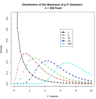
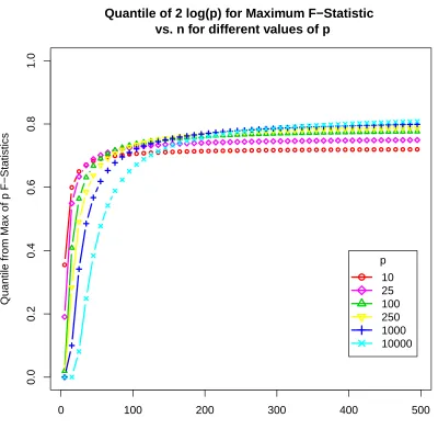
Below we show precisely what that distribution looks like for various values ofp. We

fix the number of observationsnat 100.

2_{Technically speaking, all F-statistics share the same denominator so they are not independent.}

(27)

0 2 4 6 8 10

0.0

0.1

0.2

0.3

0.4

0.5

0.6

F−Statistic

Density

1 5 10 25 100

Distribution of the Maximum of p F−Statistics n = 100 fixed

Figure 2.1: Distribution of the maximum F-statistic for p independent normal random

variables with a response y that is also a normal random variable. This represents the

maximum F to enter in a model that is pure noise.

The above figure clearly shows that our choice ofλshould be increasing in p. This

is intuitively clear since the larger our pool of variables to select from, the larger we

expect this maximum to be. The leftmost distribution corresponds to p = 1. This is the

F-distribution that all standard software packages would calculate p-values with respect

(28)

Risk Inflation Criterion makes it rigorous.

RIC:λ= 2 log(p)

George & Foster motivate the Risk Inflation Criteria (Foster and George, 1994) by

con-sidering the worst possible inflation of risk due to selection, relative to the true model.

More specifically, define the Risk Inflation (RI) as

RI( ˆβ)= sup β

EkXβ−Xβˆk2

EkXβ−Xβˆ∗_k2

where we define ˆβ∗ to be the estimated β vector if an oracle told us precisely which

coefficients are nonzero. Choosingλ=2 log(p) in the canonical variable selection

prob-lem yields a model that is minimax with respect to RI when the predictors are orthogonal.

This penalty is important. It is the first one that grows with the size of the predictor space.

As the graphs above demonstrate, this is a desirable trait. Additionally, the expected value

of the maximum F-statistic is asymptotically 2 logpmotivating this penalty even more.

This penalty also coincides with the universal threshold for wavelets developed

indepen-dently by Donoho and Johnstone (1994). Another illuminating connection is between the

RIC and the Bonferroni correction. When we are in a multiple testing framework with

ptests and seek control over the Familywise Error Rate (FWER) at levelα, we conduct

each individual test at levelα/p. If we translate theα/pquantile to the F-distribution, this

is asymptotically sandwiched for large pbetween 2 logpand 2 logp−log logp(Foster

(29)

2.1.3 λ

as a function of

p

and

k

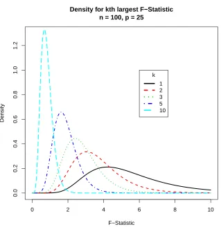
Now suppose we remove the restriction of a null model so that the βvector might have

nonzero entries and that we have added the first variable. Is it fair to penalize the next

variable by the same 2 logp penalty? If the remaining p-1 variables truly have zero

coefficients, we are now selecting an F-statistic from one of two distributions. First,

if we added the first variable correctly, then we are selecting the largest of p − 1

F-statistics. If instead we added the first variable incorrectly, then we are selecting the

2nd _{largest of} _p_{F-statistics. Additionally, each of these distributions are truncated at the}

value of the maximum F-statistic. In either case, we are selecting from a distribution that

is stochastically smaller than the largest F-statistic. The truncation only accentuates this

fact. So, intuitively, we should relax the penalty. We illustrate this graphically below.

We now ask more generally, suppose we have added k variables, how should we

penalize the addition of the (k+1)st variable.

False Discovery Rate

The penalty decreasing inkcan be motivated from an important statistical perspective –

the false discovery rate (FDR) (Benjamini and Hochberg, 1995). The false discovery rate

is a multiple testing procedure that controls the proportion of falsely rejected hypotheses.

In the variable selection context, a rejected hypothesis corresponds to adding a variable to

the model. A falsely rejected hypothesis corresponds to adding a variable that we should

(30)

0 2 4 6 8 10

0.0

0.2

0.4

0.6

0.8

1.0

1.2

Density for kth largest F−Statistic n = 100, p = 25

F−Statistic

Density

k

1 2 3 5 10

Figure 2.2: Distribution of various order statistics for the F-distribution for 100

observa-tions of 25 independent normal random variables with a response y that is also a normal

random variable. This motivates the idea whyλshould be decreasing ink.

by a smaller amount since the total number of rejections – the denominator of the FDR –

is increasing. For example, the addition of the first variable causes the FDR to be either

0 or 1 – a difference of 1; whereas the addition of the tenth variable causes the FDR to

differ by 1/10. Each variable added impacts the FDR less so we are more tolerant of an

(31)

Modern Methods: λ= 2 log(p/k)

Many of the most recently developed variable selection penalties share this trait. The

penaltyλshould be increasing in pwhile decreasing inkas we add additional variables.

Precisely, under the assumption that the number of nonzero predictors grows at a slower

asymptotic rate than the number of predictors, i.e. k=o(p), we have a family of penalties

that are approximately λ = 2 log(p/k). For the first variable, the penalty is the same as

RIC.

Foster and Stine (1999) derive the penaltyλ= 1/kPk

i=12 log(p/k) from information

theory. Assumingk =o(p), this is asymptotic to 2 log(p/k).

Tibshirani and Knight introduced the Covariance Inflation Criterion (CIC) (Tibshirani

and Knight, 1999b) which adjusts for overfitting by subtracting the average covariance

between the predicted and actual response on permuted versions of the dataset. When the

predictors are orthogonal, the penalty isλ=2/kPk

i=12 log(p/k). This penalty is twice as

large as Foster and Stine’s penalty.

George and Foster (2000) propose an Empirical Bayes approach where coefficients

are drawn from the mixture prior (1−w)δ0+w N(0,C).δ0is a point mass at 0 representing

a variable not in the model. They estimate the hyperparameters wandC from the data.

They argue that this estimator penalizes the kth variable by a quantity close to 2 log((p+

1−k)/k).

Birge and Massart (2001) studied model selection under a class of penalties including

(32)

Abramovich et al. (2005) connect asymptotic minimaxity and multiple testing for a

wide range of sparsity classes under a False Discovery Rate framework that penalizes

models closely to 2 log(p/k)

2.2 Other Variable Selection Schemes

2.2.1 L

1

methods

All of the preceding methods can be viewed in another way: regularization of theβvector

by the L0norm. That is we selectβto minimize

β∗

k,λ =arg minβ

(y−Xβ)T(y−Xβ)

σ2 +λkβk0

wherekβk₀ = Pp

i=1I(βi , 0)

As discussed above, one of the inherent difficulties of this problem is searching over

all 2p subsets which grows exponentially in p. One way to generalize this criterion is to

consider a different norm. Suppose we replace theL0norm with a generalLqnorm.

β∗

q,λ =arg minβ

(y−Xβ)T₍_y₋_Xβ₎

σ2 +λkβkq

This is exactly what is known as bridge regression (Frank and Friedman, 1993).

Com-mon specific cases correspond toq= 2: Ridge regression (Hoerl and Kennard, 1970) and

q= 1: the Lasso (Tibshirani, 1996).

We can gain additional insight by considering a few base cases. Assume that the

(33)

common methods to the ordinary least squares estimates (OLS)

1. Ridge: q=2

ˆ

βRidge

j = (1+λ)

−1β_ˆOLS j

2. Lasso: q=1

ˆ

βLasso

j = sgn( ˆβ OLS

j )(|βˆ OLS

j | −

λ

2)+

3. Subset Selection (SS): q=0

ˆ

βS S j =β

OLS j I(|βˆ

OLS j | ≥λ)

Ridge shrinks theβvector by a multiplicative factor, but never setting any coefficients

to 0. The Lasso performs soft thresholding, shrinking each coefficient towards zero by

a constant amount. If this constant is greater than ˆβj, it sets the coefficient to 0. Subset

Selection performs hard thresholding, or the “keep or kill” strategy, by either leaving

each coefficient unchanged or setting it equal to 0.

Lasso

One fact about Bridge regression is whenq≥1, this penalized criterion performs

shrink-age of theβ vector as we see with the Lasso and Ridge penalties. The literature on the

benefits of shrinkage is vast. See (Stein and James, 1961; Lehmann et al., 1998) for its

origins in estimating the sample mean. For many shrinkage examples in modern statistics

where shrinkage improves prediction, see (Hastie et al., 2001). An additional benefit is

(34)

finding the “best” subset is NP-hard. Changing to a convex penalty, the solution is more

easily found through widely available convex optimization software. For a good

refer-ence on convex optimization see Boyd and Vandenberghe (2004).

On the other hand, Bridge regression whenq≤ 1, performs selection of theβvector,

setting some coefficients equal to 0. The Lasso withq = 1 sits right at the boundary of

these two operations. In fact, that is what Lasso stands for: Least Absolute Shrinkage

and Selection Operator. The Lasso can be viewed as the closest convex approximation

to the variable selection problem, replacing theL0 norm with theL1norm. Additionally,

the L1 penalty is continuous so that we are able to see the entire profile of regression

coefficients as we vary the penalty λ. At the two extremes, λ = 0 yields the full OLS

model whileλ=∞yields the null model. Figure 2.3 is an example. We also include the

more common Lasso coefficient profile where the x-axis is the fraction relative to the full

OLS fit.

Least Angle Regression

Least Angle Regression (LARS) (Efron et al., 2004) is one of the most fascinating recent

developments in the linear model literature. LARS can be viewed as a smooth, continuous

less-greedy version of Forward Selection. Forward Selection and LARS both start by

selecting the variable that is most correlated with the response. Where they differ is how

much they move in that direction. Forward Selection moves along that direction until

(35)

0 200 400 600 800 1000

−20

−10

0

10

20

Regression Coefficients for values of lambda

lambda

Coefficients

0.0 0.2 0.4 0.6 0.8 1.0

−20

−10

0

10

20

Regression Coefficients for fractions of OLS fit

|beta|/max|beta|

Coefficients

Figure 2.3: Coefficient profile for the Lasso as we varyλon the left, and as we vary the

fraction relative to the full OLS fit on the right. This is the diabetes data taken from Efron

et. al (2004)

direction until we reach a point where another variable is equally correlated, we stop and

change directions to the one that is equiangular to the two equally correlated variables.

This is best illustrated with a geometric example.

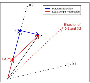
We have a response variableywith two predictor variables X1andX2. The variable

most correlated withyis equivalent to the variable which forms the smallest angle with

it. In this case, we selectX2first. Both Forward Selection (FS) and LARS proceed in this

direction. They differ by how far they travel.

Here we see the precise path that FS and LARS take. Forward Selection proceeds

along X2 until the residual vector is orthogonal to it. It then moves in this orthogonal

(36)

X1

X2

y

●

Bisector of

X1 and X2

LARS

FS

Forward Selection Least Angle Regression

Forward Selection vs. Least Angle Regression

Figure 2.4: Both Forward Selection and Least Angle Regression selectX2as the direction

to move. Forward Selection travels until the residual vector is orthogonal. Least Angle

Regression travels to the point where the residual vector is equally correlated withX1and

(37)

residual vector is equally correlated – equivalently forms the same angle – with X1 and

X2. It then proceeds in the direction equiangular toX1andX2 – the angle bisector.

Un-fortunately, we can only view this in two dimensions but the LARS algorithm generalizes

to more than two directions. We add a new variable to the model each time its correlation

with the current residual vector matches the correlation with those variables already in

the model. We then recompute the equiangular direction with the new variable added,

and proceed in that direction. LARS, just like Forward Selection, eventually reaches the

Ordinary Least Squares (OLS) solution. It just does so in a less greedy manner. The

geometric reasoning behind LARS is what gives it its name. At any given point in the

algorithm, those variables that form the least angle with the current residual vector are

included in the model. Any variables forming a larger angle are excluded.

Even more remarkable, with slight modifications of the algorithm, we can derive the

entire path of Lasso solutions and the infinitesimal forward stagewise solutions. We point

the interested reader to the original paper (Efron et al., 2004) and to a follow-up equating

Lasso and Forward Stagewise in an expanded predictor space (Hastie et al., 2007).

Dantzig Selector

The Dantzig Selector (Candes and Tao, 2007) is a recent development especially suited to

the p> ncase, where we can recover the nonzero components of theβvector with large

(38)

Selector is defined to be the solution to the convex problem

min β∈Rp

kβkl1 subject to

X

t

r

_l_∞ ≤ λσ

wherer =y−Xβis the residual vector. They recommendλ= p2 logp, which coincides

with the RIC penalty. Candes and Tao showed that the program can be recast as a linear

program, speeding up computation time. A remarkable result is that the mean squared

error of β is within a logarithmic factor of the mean squared error if an oracle told us

precisely which coefficients were nonzero. This result is not asymptotic. We should

note the mean squared error above is for the βvector, not the Xβ vector for prediction.

Efron et al. (2007) show the predictive performance of the Dantzig Selector relative to the

Lasso to be similar in some cases and inferior in others. In the rejoinder, Candes and Tao

specifically note the applications in biomedical imaging, genomics, and data conversion

where estimatingβis paramount.

2.2.2 Data Resampling Methods

Resampling methods attack variable selection from a different perspective by sampling

repeatedly from the data to mimic what would happen with new data.

Cross Validation

The fundamental idea behind cross-validation (CV) is to divide the data into two parts and

use the first part to build the model and the second part to evalute the fit. We generally

(39)

nearly equal) parts. We denote these parts by Γ1, . . .ΓK and let Γ(k) be the data with

Γk deleted, k = 1, . . . ,K. Suppose we have a sequence of forward selection models

M0,M1, . . .MpwithMjthe model with jvariables. Then for eachk, we carry out forward

selection on Γ(k) generating models M₀k,M₁k. . .Mkp with respective sizes 0,1, . . .p. Note

that there is no reason forMk

j to have the same jvariables as Mjsince Forward Selection

may select different variables on different subsets. Then for each model sizejwe evaluate

its cross-validated error (CVc) as

c

CV(j)= 1

n

K

X

k=1 X

(yi,xi)∈Γk

(yi−µˆk(xi,Mkj)) 2

where ˆµk is the predictand evaluated on the left out subsetΓk under model Mk_j.

We select model sizek = arg minjCVc(j). Stone (1977) showed that leave-one-out

cross-validation (K = n) is asymptotically equivalent to AIC. However, Breiman and

Spector (1992) recommend five-fold cross validation for variable selection based on

sim-ulation results because leave-one-out CV tends to select the same model as the entire data

too often.

Both leave-one-out and five-fold CV are inconsistent for model selection. Shao

(1993) showed that they tend to include too many variables. He proves we can ensure

model consistency by letting the number of observations left out nv satisfynv/n → 1 as

(40)

Bootstrap

The bootstrap attacks the variable selection problem by sampling with replacement from

the empirical distribution. The bootstrap is typically applied in one of two ways. First,

we can bootstrap the residuals. We start by fitting the full model estimating regression

coefficients ˆβand the residualsei, i= 1, . . .n. We then studentize the residuals defined by

e∗_i =ei/

√

1−hi wherehi is theith diagonal element of the hat matrixH =X(XTX)−1XT.

We then generate for each observation, a new y∗_j = xjβˆ + e∗j where e

∗

j is sampled with

replacement from the studentized residuals. Crucial to bootstrapping residuals is that

they have constant variance. This method is suitable if we treatXas fixed.

Second, we can bootstrap by sampling with replacement from the observed (xi,yi)

pairs. This method is appealing if we are working in the random-Xcase. It also makes

no assumptions on the model, unlike the homoscedastic error assumption above.

Conse-quently, we can view bootstrapping (x,y) pairs as “more nonparametric” than

bootstrap-ping residuals. One problem that may arise in the p > ncase is each bootstrapped data

set has rank on average about 63% as large as the original data set.

Shao (1996) showed that this bootstrap scheme is not consistent. If we bootstrap

residuals, we can ensure consistency by increasing the variability of the residuals. If

we bootstrap pairs, we can ensure consistency by constructing smaller bootstrap samples

with size nb with nb/n → 0 asn → ∞. For a thorough treatment of the bootstrap see

(41)

Little Bootstrap

Breiman (1992) introduced the little bootstrap as an alternative toCp that does not suffer

from such severe selection bias. Suppose we fit a model with j coefficients denoted ˆµj.

The model error can be written as

ME( ˆµj)=kµ−µˆjk2 =RSSj−RSSp+kµ−µˆpk2−2(,µˆp−µˆj)

where the subscript pdenotes the full model with all predictors included and (·,·) is

the inner product. We also estimate the residual variance from the full model fit ˆµp. The

first two RSS terms are directly computed. We can estimatekµ−µˆpk2as pσˆ2 assuming

the full model has no bias. We need an estimate for this last term. Breiman proposes the

little bootstrap to estimate this term. We generate bootstrapped responses as

˜

yi =yi+˜i where ˜i ∼N(0,t2σˆ2)

Note that we add the error term to the original responseyand not the predicted response

ˆ

ylike the residual bootstrap of the previous section. We then fit the model using forward

selection to the (˜yi,xi) pairs with jvariables and all pvariables as above. Call these fits

˜

µjand ˜µp. We then calculate

1

t2(˜,µ˜p−µ˜j)

Repeat this Btimes and average. Breiman showed that

1

t2E(˜,µ˜p−µ˜j)≈ E(,µˆp−µˆj)

(42)

expression above.

d

ME( ˆµj)=RSSj−RSSp+ pσˆ2−

2

B

X

b=1

(˜b,µ˜b_p−µ˜b_j)

where the superscript bcorresponds to a particular bootstrap sample. Based on

simula-tions, Breiman recommends t = 0.6 and B = 40. The best model is then chosen with

respect to this model error estimate.

2.2.3 Bayesian Methods

The Bayesian view on variable selection has seen a great deal of research in the past two

decades. The fully Bayesian approach is as follows. Suppose that we have 2p models

denoted by M1,M2, . . . ,M2p each of which corresponds to a distinct subset of the

vari-ables{X1,X2, . . .Xp}. We need two prior probabilities. First, we need a prior probability

for the model Mγ which we denoteπ(Mγ) and given the model, we need priors for each

regression coefficient, denoted byπ(βj|Mγ), j =1,2, . . .p. The posterior probability for

model Mγis given by

π(Mγ|y,X)= pγ

(y|X)π(Mγ)

P2p

k=1pk(y|X)π(Mk)

where

pγ(y|X)= Z

p(y|βγ,X)πγ(βγ|Mγ)dβγ

Selection occurs based on these posterior probabilities. The clear obstacle is then

how do we choose the priors. Mitchell and Beauchamp (1988) introduced “spike and

(43)

(the spike) and a uniform distribution between −c andcfor some constant c (the slab).

One obvious drawback is the finite support of the prior. One common alternative is to put

normal priors on those variables appearing in the model. For the model itself, we put a

binomial probability

P(Mγ)= wk(1−w)p−k

where k is the number of variables in modelMγ. With this setup and fixingσ2, Chipman

et al. (2001) showed that under different parameterizations, we can generate the variable

selection problem for any penalty λ(e.g. AIC, BIC, RIC). Berger and Pericchi (1996)

take a different approach, similar to cross-validation, by proposing to use part of the data

to estimate the prior distributions and the remaining data to generate posterior

probabili-ties.

Research prior to the advent of Markov Chain Monte Carlo (MCMC) methods

fo-cused on developing priors that minimally influence the posterior. The development of

MCMC methods shifted the attention to fully specified prior distributions. The use of

MCMC allows for much easier posterior calculations. Consequently, the primary

obsta-cle now is how to intelligently search through the posterior. Markov Chain Monte Carlo

model composition (MC3) (Madigan et al., 1995; Raftery et al., 1997) proceeds similarly

to Efroymson’s stepwise algorithm. We start with a random subset of the variables. At

each step, just like stepwise, we either add or delete a variable. The key difference is the

choice of what variable to add or delete is stochastically guided. An alternative to MC3

(44)

allowing a mixture of two normal distributions, one with a very small variance. If the

regression coefficient is sampled from this distribution, we can safely say its coefficient

is 0 and should be left out of the model.

A related line of research in this context is Bayesian Model Averaging (Hoeting et al.,

1999) where we take a weighted average of models sampled by the posterior. While this

often gives better predictions, we lose our parsimonious goal of variable selection. Most

or all variables will appear in the averaged model. For a general overview of Bayesian

methods, see (Gelman et al., 2004).

2.3 False Selection Rate

We now discuss the the False Selection Rate (FSR) (Wu et al., 2007), a variable selection

scheme most similar to the one we propose in the next chapter. We develop the FSR in

detail in this section so that later we can contrast specific points with our method. We

define the important variables as those for which βj , 0 and unimportant variables as

those for which βj = 0. Ideally, we select all important variables and no unimportant

variables. The FSR attempts to control the proportion of falsely selected unimportant

variables. Suppose we specify an F-to-enter value that corresponds to significance level

α and perform forward selection. The model selects k(α) variables of which kI(α) are

important andkU(α) are unimportant. kU(α)+kI(α)=k(α). We of course do not observe

(45)

of falsely selected variables, given by

γ(α)=E kU(α)

1+k(α) !

We add 1 to the denominator to account for the intercept which is typically forced

in the model and to avoid division by zero. In their paper, Wu, et al. consider two

definitions, one the expectation of the ratio and another the ratio of expectations. We

focus on the expectation of the ratio as it is the one they use in their simulations. The key

goal is to select α∗ so that γ(α∗) = γ0 for some prespecified false selection rateγ0. To

ensure uniqueness, we take

α∗= sup{α:γ(α)≤ γ0}

For example, (kI,kU)=(3,1) and (kI,kU)= (7,2) both give an FSR of 0.2. We prefer the

larger model.

To control the FSR, they augment the predictor space with pseudo-variables that by

design have no relation to the response. Consequently, by monitoring the number of

pseudo-variables selected, and under the assumption that the pseudo-variables behave

like the unimportant real predictors, we can estimate the FSR. We make our notation

precise. Whenever we use p we mean the total number of predictors. If we attach a

subscript to p, we mean the total number of predictors of that type, e.g. pI is the total

number of important predictors, pU unimportant. We also introduceZ to be the

pseudo-predictors. Consequently, we have a total of p = pI + pU + pZ predictors and at entry

(46)

to control

γ(α)= kU(α) 1+kU(α)+kI(α)

The denominator does not need to be estimated since we know how many total

vari-ables we selected k(α) and we know how many of those are pseudo-predictorskZ(α), so

the denominator is simply 1 +k(α) −kZ(α). The numerator requires more effort. We

need to make an assumption that on average the proportion of selected unimportant real

predictors is equal to the proportion of selected pseudo-predictors for allα. That is,

EkU(α)

pU

=EkZ(α)

pZ

and if we solve forkU(α), we get

kU(α)=

pU

pZ

kZ(α)

Unfortunately, we also do not know pU. So, we take an optimistic estimate and assume

that among real predictors selected, we only selected important ones, i.e. kU(α)= 0. That

is

ˆ

pU = pU+ pI −kU(α)−kI(α)= p− pZ+k(α)−kZ(α)

Every quantity on the right hand side is directly observable. In practice, we repeat

this many times, generating new pseudo-variables and taking averages to estimate ˆpU,

k(α), andkZ(α). Wu et al. use B=500. We denote these averages as ¯ˆpU, ¯k(α) and ¯kZ(α),

respectively.

We now have our estimate of the FSR

ˆ

(47)

We then select

α∗∗ = sup{α: ˆγ(α)≤γ0}

Note that we estimateα∗∗from the augmented space with pseudo-predictors and that

it does not coincide with α∗estimated from the actual data. The final model is selected

by running forward selection with a p-to-enter ofα∗∗ on the real data.

One key issue we postponed until now involves the pseudo-variables. Namely, how

many of them do we include and how do we generate them? Wu et al. propose four

different methods.

1. Generate independent normal variables

2. Randomly permute the rows ofX

3. Generate independent normal variables and orthogonalize with respect toX

4. Randomly permute the rows ofXand orthogonalize with respect toX

The last two methods are simply the first two methods adjusted to ensure that every

pseudo-variable has zero correlation with every real predictor. The last two methods can

not be used in the case p > n, and also suffer in the case p > n/2 since the rank of the

pseudo-variables is at mostn− pwhich is smaller than the rank ofX. Methods 2 and 4

also restrict the number of pseudo-variables to be precisely the same as the number of real

variables pZ = pI +pU. In their simulations results, Wu et al. selected the fourth method

based on simulations. We will have more to say about the generation of pseudo-variables

(48)

Chapter 3 Permuted Inclusion Criterion

We now get into the heart of this thesis, describing the data augmentation procedure and

how we apply our variable selection scheme. We will show that in the univariate case,

our method coincides with Pitman’s classic permutation test. We will then go into detail

about how to adjust our predictors after each step of Forward Selection. In the last section

of this chapter, we will compare and contrast our method with the False Selection Rate.

3.1 Augmenting the Data by Permutation

Our procedure begins by augmenting the predictor spaceX, which we will call the actual

or real data with a copy of X, denotedXπ, in which the rows have been randomly

per-muted. We will call Xπ the permuted data or the fake data. We now have an augmented

predictor spaceXe= X|Xπwhich consists ofnobservations on 2pvariables. For each

(49)

the same marginal distributions since we only permuted the data. Additionally, if we let

var(X)=S,

var(X)=var(Xπ)=S

The covariance structure is exactly the same, because the inner products are left

un-changed. This is an extremely desirable property for variable selection because the

dis-tribution of test statistics depends on the correlation structure of the data. Furthermore,

Xπpreserves transformations and interactions between other variables. For example,

sup-poseX3 =X2·X1, thenXπ3= Xπ2·Xπ1. Lastly, a trivial yet important observation is that

Xπ scales with the size ofX. Both have pvariables. The larger the pool of predictor

vari-ables to select from, the larger the pool of fake predictors to penalize variable selection.

This coincides with the intuition of RIC that the penaltyλshould be increasing in p.

3.2 Forward Selection with the PIC

Forward Selection proceeds in a greedy fashion. We start out with the null model with

no predictors selected. Then at each step, we select the variable most correlated with

the current residual vector. Now suppose that instead of selecting the most correlated

predictor fromX, we select the most correlated predictor from the augmented dataeX. As

long as we have not yet chosen a permuted predictor fromXπ, this procedure is equivalent

to selecting fromX, since the order of variable entry is fixed conditional on observingX.

We propose a simple stopping criterion: as soon as we would select a predictor fromXπ,

(50)

the realized permutation. Thus, we will simulate many permutations and create an entire

distribution of model sizes to select our final model. Ideally, we would sample from all

n! permutations. However, this is prohibitively large for moderate n, so we simulateN

times. This seemingly ad-hoc stopping criterion possesses many sensible properties.

Suppose we have the null hypothesis thaty is a complete noise model: y = . Now

consider selecting from X and from Xπ separately. For X we select the variable with

the largest absolute correlation from a pool of ppredictors with covariance matrixSthat

has no relation to the response under the null hypothesis. ForXπ we select the variable

with the largest absolute correlation from a pool of ppredictors with covariance matrix

S that has no relation to the response because we broke the relationship by permuting.

They only differ in the reasons why they have no relationship with the responsey– one

hypothetical under the null hypothesis, and one actual because we manipulated the data

through permutation. If the largest absolute correlation from Xis larger than the largest

absolute correlation fromXπ, we add that variable to the model. Otherwise, we stop and

select the null model. Under the null hypothesis, we would expect the choice betweenX

andXπto be equally likely.

Before we delve into the details of how to adjust the variables and select a model, we

(51)

3.3 PIC applied to a single predictor

Suppose we have a single predictor variable denoted by lowercase x, and its permuted

analog byxπ. If we adopt the forward selection framework, we have two possible models

M0 :y= or M1 :xβ+

For a given permutationπ, we selectM0if|cor(y,xπ)|> |cor(y,x)|. Otherwise, we

se-lectM1. Suppose we now takeN total permutations and letπj denote the jthpermutation.

We sample πj from the universe of all n! permutations, which we denoteΠn. LetC0be

the count for the number of times we select M0. We have the following algorithm.

Result: Permuted Selection with a Single Predictor

We initializeN total permutations, and count variableC0 =0

fori=1toNdo

Sampleπj fromΠn

if|cor(y,xπj)| ≥ |cor(y,x)|then

SelectM0

C0←C0+1

else

SelectM1

end

Algorithm 2: Permuted Inclusion Criterion: Single Predictor Variable. We augment

the predictor space with xπj and we count the number of times that it has a larger

(52)

This looks strikingly familiar to the permutation test for correlation betweenxandy

(Pitman, 1937). In fact, let

ˆ

P= C0+1 N+1

then ˆP is the P-value for the test of correlation between x andy. This P-value is exact

up to simulation error and does not depend on the error distribution. The only fact we

need is independent data. We add one to the numerator and denominator because the

observed correlation is typically included in the reference set. Under the null hypothesis,

C0 is uniformly distributed on the integers {0,1, . . .N}. This connection should not be

surprising since adding a variable to the model is equivalent to testing whether its slope

is 0, and testing whether a slope is 0 is equivalent to testing whether its correlation is

0. We often view a permutation test for correlation by considering many realizations

of xπ alone, not augmented with x. However, we see that this alternative framework of

augmenting the data and then selecting is equivalent for the single predictor case. Before

we extend the PIC to the multivariate case, we develop some notation.

3.4 Permutation Framework

We defineΠto be the space of all row permutations. Note

|Π|=n!

We suppress the dependence onnsince we typically view the number of observations as

(53)

ofX.

Different realizations ofXπ will give different stopping points for Forward Selection.

We defineΠjto be the subset ofΠsuch that we have not stopped after jsteps. That is, we

have yet to select a variable from Xπ after jvariables have been selected. For example,

Π2 corresponds to those permutations where the first two variables selected came from

X. Since we stop the first time we select fromXπ, we have the relation that

Π= Π0⊇ Π1⊇ Π2. . .⊇Πp ⊇Πp+1 =∅

Clearly,Π0consists of all the permutations since we have not selected any variables yet.

Also, since we have preal variables to select from,Πp+1corresponds to the empty set.

3.5 The Multivariate Case

Until now, we avoided an important issue with forward selection. Recall that in

tradi-tional forward selection, we adjust not only the current residual vector but also all other

predictors yet to enter the model. We now examine how to adjust the augmented space

e

Xand how it impacts the selection of later variables. We adopt notation from chapter 1.

LetXj

andXπj denote the real and permuted spaces after we adjust for the first jvariables

entered in FS.

We have three desired goals with PIC.

1. At each step in the algorithm, we wantvar(Xj₎₌

(54)

2. AssumingXj has no signal to explain the response, the choice betweenXj andXπj

is equally likely

3. At step j,Xπj corresponds to a permutationπ ∈Πj

We mention these three goals because unfortunately, we will only be able to

simul-taneously satisfy at most 2 of these goals for different adjustment schemes. We desire

the first goal because one of the main motivations for the PIC over traditional methods

is that it adapts to the covariance structure of X. This means the F statistics have the

same correlations throughout all steps of forward selection. Traditional selection criteria

mentioned in chapter 2 do not address correlated test statistics. We already mentioned

the benefit of augmenting with permuted data is that var(X) = var(Xπ). This is true at

the start of the algorithm. However, as we proceed with Forward Selection this may not

continue to hold. It depends on how we adjust.

We desire the second goal because under the assumption that Xj posseses no more

signal to explain the current residual vector, we should be indifferent betweenXandXπ.

We desire the third goal because we want to be sampling from the right subset. For

example, why would we consider adding a 4th variable if we already stopped after the

2nd variable. This goal essentially prevents us from re-permuting at each step of Forward

Selection.

We adopt the notation X2:1 to mean X2 adjusted for X1. In regression terms, this

means we regressX2onX1and take the residuals. This is the part ofX2that is orthogonal

Permuted Inclusion Criterion: A Variable Selection Technique

University of Pennsylvania

ScholarlyCommons

Permuted Inclusion Criterion: A Variable Selection

Technique

Shaun Lysen

Permuted Inclusion Criterion: A Variable Selection Technique

Permuted Inclusion Criterion: A Variable Selection Technique

Shaun Lysen

A Dissertation

in

Statistics

Presented to the Faculties of the University of Pennsylvania in Partial

Ful-fillment of the Requirements for the Degree of Doctor of Philosophy

2009

Andreas Buja

Supervisor of Dissertation

Eric Bradlow

Acknowledgments

Contents

Chapter 1

Introduction

1.1

The Need for Variable Selection

1.2

Variable Selection in Linear Regression

1.3

Building Candidate Models – Common Algorithms

1.3.1

All Subsets

1.3.2

Stepwise Methods

Chapter 2

Selection Criteria – When To Stop?

2.1

The Need for a Penalty

2.1.1

Constant

λ

2.1.2

λ

as a function of

p

2.1.3

λ

as a function of

p

and

k

2.2

Other Variable Selection Schemes

2.2.1

L

methods

X1

X2

y

Bisector of

X1 and X2

LARS

FS

2.2.2

Data Resampling Methods

2.2.3

Bayesian Methods

2.3

False Selection Rate

Chapter 3

Permuted Inclusion Criterion

3.1

Augmenting the Data by Permutation

3.2

Forward Selection with the PIC

3.3

PIC applied to a single predictor

3.4

Permutation Framework

3.5

The Multivariate Case