A STANDARDIZED QUANTIFICATION TECHNIQUE FOR EVALUATION, INTERPRETATION OF DE-MRI SCANS

International Journal of Advanced Technology in Engineering and Science www.ijates.com

Volume No 03, Special Issue No. 01, March 2015 ISSN (online): 2348 – 7550

1077 |

P a g e

A STANDARDIZED QUANTIFICATION TECHNIQUE

FOR EVALUATION, INTERPRETATION OF DE-MRI

SCANS

Nasreen Sulthana.D

,

Asif Hussain.S

1

M.Tech Scholar,

Associate Professor, E.C.E, AITS, Rajampet, Andhra Pradesh, (India)

ABSTRACT

Delayed-enhancement magnetic resonance imaging (DE-MRI) is an effective technique for detecting left atrial (LA) fibrosis both pre and postradiofrequency ablation for the treatment of atrialfibrillation. Fixed thresholding models are frequently utilized clinically to segment and quantify scar in DE-MRI due to their simplicity. These methods fail to provide a standardized quantification due to inter- observer variability. Quantification of scar can be used as an endpoint in clinical studies and therefore standardization is important. In this paper, we propose a segmentation algorithm for LA fibrosis quantification and investigate its performance. The algorithm was validated using numerical phantoms and 15 clinical data sets from patients undergoing LA ablation. We demonstrate that the approach produces good concordance with expert manual delineations. The method offers a standardized quantification technique for evaluation and interpretation of DE-MRI scans.

Keywords: Delayed-Enhancement MRI, Left Atrium, Image Segmentation, Fibrosis.

I. INTRODUCTION

Atrial fibrillation (AF) affects approximately 2.3 million people in the USA with significant co morbidity and

mortality[1], [2]. It is a condition that increases the risk of stroke by a factor of six-fold and doubles the

mortality rate of patients when compared to age-matched controls. Since it was shown that ectopic beats from

the pulmonary veins (PV) give rise to AF [3] the treatment of AF using radiofrequency catheter ablation

(RFCA) has become an important and common procedure. In this procedure, ablation lesions are created in a

circular fashion around the PV Ostia to electrically isolate the PVs, and thus the ectopic focal points, from the

rest of the left atrium (LA). This treatment can provide a cure for the majority of patients and prevent the

requirement for long-term pharmacotherapy. However, for a high proportion of patients (15%_46%) [4]_[6],

there is recurrence of AF. This normally requires a second or third re-do ablation procedure and thus has a high

burden on health care. It is important to select patients who will respond better to RFCA to reduce recurrence

rates. Several studies have shown that it is possible to predict the outcome of RFCA procedures from the fibrosis

extent in LA [7]_[10]. A scoring system based on the degree of fibrosis has been developed, leading to

treatment stratification [8]. Other recent studies have also highlighted the significance of the extent of fibrosis or

scar in LA post-ablation for predicting outcome [11], evaluate effectiveness of ablation technologies [12] and

helping to gain a better understanding of the left atrial substrate [13].In this context, magnetic resonance

imaging (MRI) has been shown to be effective for non-invasive imaging of the LA .In particular, Gadolinium

post-International Journal of Advanced Technology in Engineering and Science www.ijates.com

Volume No 03, Special Issue No. 01, March 2015 ISSN (online): 2348 – 7550

1078 |

P a g e

RFCA [8]. DE-MRI is acquired with an inversion recovery gradient echo sequence performed after

administration of Gadolinium yielding an image at an inversion time which is chosen to null the signal from

healthy myocardium. Due to the differential washout kinetics of Gadolinium, scar or fibrotic areas are

differentiated from healthy tissue. Fibrotic or scar tissues in the myocardium appear with a signal intensity (SI)

above normal myocardium. Fig. 1 shows some examples of DE-MRI with intensities significantly higher than

myocardium.

Fig 1

.

DE-MRI images from three separate patients taken 3 months post-ablation. Arrows

indicate areas of enhancement. Abbreviations: AO - aorta, LA - left atrium

.

Quantification of scar or fibrosis from DE-MRI is challenging due to various reasons [14]. The thin myocardium

of the LA wall leads to low signal-to-noise ratio. Contrast variation in these images can be an issue due to

choice of inversion time. Also the complex geometry of the LA results in some transverse slices where a very

small section of the anatomy is visible, making manual quantification in these areas highly observer dependent.

Finally, patients suffering from AF often have an irregular heart rate and breathing making it hard to

acquire good quality respiratory- and cardiac-gated images. Quantification from such images become difficult to

auto-mate and manual quantification tends to be highly observer- dependent. In this work, a scar quantification

approach is proposed and investigated. The method exploits a well-known image segmentation approach known

as graph-cuts [15]. Segmentation is achieved using a combination of scar intensity model priors and

Gaussian-tting to tissues in the unseen image to be segmented. The final labelling is achieved by optimizing a cost

function using graph-cuts.

1.1 Previous Works

Quantification and segmentation of ventricular scar from DE-MRI images have been studied in several

investigations. Refer to Table 1 for a brief summary. A common method for detecting scar or fibrosis is to use a

fixed model of thresholding between two and six standard deviations (SD) above the mean intensity of healthy

myocardium [16]_[19]. This requires the user to manually outline remote or healthy myocardium. Another

common method is the Full-Width- At-Half-Maximum (FWHM) which sets scar to be intensities greater than

50% of manually outlined hyper-enhanced myocardium [19]. Other approaches exist to compute the threshold

International Journal of Advanced Technology in Engineering and Science www.ijates.com

Volume No 03, Special Issue No. 01, March 2015 ISSN (online): 2348 – 7550

1079 |

P a g e

surface-based segmentation [23] and threshold- surface-based volumetric segmentation [7], [14], [24]. In [23], the maximum

intensity projection (MIP) of the DE-MRI SI on the segmented LA shell is used to visualize enhancing

intensities on the surface. This technique has an important drawback: it is only a visualization of intensities and

thus not a segmentation technique with no volumetric segmentation as output. In [7], a volumetric segmentation

of pre-ablation LA fibrosisis proposed by obtaining suitable measurements from the intensity histogram within

atrial wall. This has a disadvantage that the LA wall is thin and thus its manual segmentation can have

significant inter-observer variation. Other methods have employed fixed models for pre-ablation fibrosis [24]

and post-ablation scar [25] with variable thresholding. In summary, a fixed thresholding model cannot handle all

the different variabilities encountered in LA DE-MRI and these are both from the varied internal factors (size,

distribution and heterogeneity of scar) and varied external factors (resolution, image noise, inversion time,

surface coil intensity variation). The inversion time choice can generate the appearance of more or less scar, and

change the appropriate scar threshold. Motion blurring also reduces the appearance of scar.

1.2 Contributions

In this work, we present a method for segmenting and thus quantifying LA fibrosis in DE-MRI. It is based on a

probabilistic tissue intensity model of DE-MRI data, which is derived from both training and the unseen data. It

offers two advantages: 1) It does not require manual outlining of base-line healthy myocardium, and 2) It

provides greater accuracy than fixed models with no inter-observer variation. The algorithm was evaluated and

compared with existing clinically-used methods using local pixel overlap measures. Performance was analyzed

by exploring various scar contrast levels. An abbreviated version of this work was published in

[31] and [32]. In this current version, we present the approach with more details including additional

experiments and validation. We also include an automated adaptive step that allows for variation in the scar

signal level and avoids sub optimal scar intensity models. Furthermore, we present a much more comprehensive

validation of the algorithm on a larger clinical cohort. The algorithm was also used recently in a segmentation

challenge [33], segmenting sixty DE-MRI datasets from three imaging centres.

II. CLINICAL AND IMAGING PROTOCOLS

2.1 Patients

15 patients were followed up at 6 months following their first ablation for the treatment of paroxysmal AF. The

procedures were carried out in the cardiac catheterization laboratory at St. Thomas Hospital, London, U.K. All

patients gave writ- ten permission to take part in this local ethics committee

Approved study.

2.2 Ablation Procedure

A catheter was placed in the coronary sinus to provide a reference for electro anatomic mapping and to enable

LA pacing. Two transept punctures were made to access the LA using standard long sheaths (St. Jude Medical,

International Journal of Advanced Technology in Engineering and Science www.ijates.com

Volume No 03, Special Issue No. 01, March 2015 ISSN (online): 2348 – 7550

1080 |

P a g e

placed in each PV in turn while the corresponding LA-PV ostium was targeted with wide area circumferential

ablation. Energy was delivered through a 3.5 mm irrigated tip catheter with _ow limited to 17 ml/min, power

limited to 30 W on the anterior wall and 20 W on the posterior wall and temperature limited to 50_C. Ablation

lesions were marked on the LA geometry when there had been an 80% reduction in the local electrogram

voltage or after 30 seconds of energy delivery. The clinical endpoint was electrical isolation of all PVs.

2.3 MRI Scanning Procedure

MRI scanning was performed before and after the ablation procedure. Pre-ablation scanning was performed 24

hours prior to the procedure and post-ablation scanning was per- formed 6 months after the procedure. The

proposed algorithm in this work was developed and evaluated primarily for post ablation images. All scanning

was performed on a 1.5T Achieva scanner (Philips Healthcare, The Netherlands). The examination began with a

survey and reference scans, and an interactive scan to determine the four-chamber orientation of the heart. For

anatomical information, a 3D magnetic resonance angiography (MRA) scan with whole-heart coverage

(1_1_2mm3 acquired, 1_1_1mm3 reconstructed, 20 secs duration) was acquired following the injection of 0.4

ml/kg double dose of a gadolinium-diethylenetriaminepentaacetate (Gd-DTPA) contrast agent. This scan was

not cardiac-gated. This scan was followed by a 3D respiratory navigated and cardiac-gated, 3D balanced

steady-state free precession (b-SSFP) acquisition in a sagittal orientation with whole- heart coverage (1:3 _ 1:3 _

2:6mm3 acquired, 1:3 _ 1:3 _ 1:3mm3 reconstructed, 6 mins duration). The scan for the visualization of

delayed-enhancement was a 3D ECG-triggered, free breathing inversion recovery (IR) turbo eldecho (TFE) with

respiratory-navigated and cardiac-gated with whole heart coverage (0:6 _ 0:6 _ 4mm3 acquired, 0:6_0:6_ 2mm3

reconstructed, 3 mins duration). Data were acquired within a window of 150 ms every one RR interval, with a

low-high k-space ordering and spatial pre-saturation

with inversion recovery (SPIR) fat suppression. The IR time delay was determined from the Look Locker

sequence, and was set at an inversion time (TI) intermediate between the optimal TIs to null myocardium and

blood. This scan was performed approximately 20 mins after contrast administration. The slices were set for

complete coverage of both left and right atria. Slice orientation was in the four-chamber view for AF ablation to

optimize visualization of the pulmonary veins.Note that the scan times quoted above are actual scan times.

Typical respiratory gating efficiency is 50% but this varies considerably in this particular patient population.

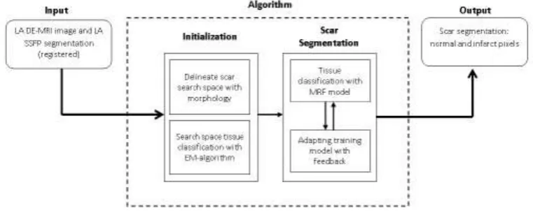
2.4 Segmentation Algorithm

Fig. 2 shows an overview of the algorithm. The inputs were a DE-MRI image and a segmentation of the LA

from an anatomical scan. The LA segmentation was obtained from the b-SSFP whole-heart scan by an

automatic approach based on a statistical shape model [34], and was followed where necessary by manual

correction by a human rater (throughout this paper, the terms human rater or observer refer to someone who has

experience viewing tomographic images and can correctly identify the LA endocardium and fibrosis in the LA

myocardium). The b-SSFP image was chosen over MRA as it was acquired at the same phase in the cardiac

International Journal of Advanced Technology in Engineering and Science www.ijates.com

Volume No 03, Special Issue No. 01, March 2015 ISSN (online): 2348 – 7550

1081 |

P a g e

were registered to the DE images using the DICOM header data, and then refined by rigid and affine registration

steps [35]. Affine registration was necessary to account for the differing PV angles in the scans. This defined the

endocardial LA boundary in the DE images.

FIGURE 2

.

An overview of the steps involved in the segmentation process. The pipeline takes as

input MRI images and outputs binary segmentations (rounded boxes). The processing pipeline

is illustrated here with each separate stage in the algorithm. Smaller boxes represent sub-stages.

The scar segmentation stage is iterative as indicated by the bi-directional arrows.

2.5 Scar Segmentation

Segmentation of scars from DE-MRI images can be defined as assigning a label fp €{non-scar; scar} for every voxel p in the search space of the image. The search space is defined as a region _3 mm from the endocardial border obtained from the atrial geometry extraction. This is within the limits of atrial wall [23]. Given the

observed intensities in the atrial wall and prior knowledge of scars, the segmentation problem is solved using a

probabilistic framework where the maximum a posteriori (MAP) estimate is computed using Bayes' theorem:

Arg max p(f/I)=(p(I/f) p(f))/p(I)

F

where f is the total label configuration and I are all observed intensities in the image. The image likelihood

p(I/f) describes how likely is the observed image given a label configuration f. The prior p(f) encodes any prior knowledge of the healthy and scar tissue classes.

2.6 Intensity Models

International Journal of Advanced Technology in Engineering and Science www.ijates.com

Volume No 03, Special Issue No. 01, March 2015 ISSN (online): 2348 – 7550

1082 |

P a g e

We first consider the intensity energy contribution from the scar tissue class, i.e. for the function p(I/fp = 1) and then for the non-scar class.

2.7 Smoothness Constraint

To ensure smoothness and avoid discontinuities in the final segmentation, the Eprior term of the MRF energy function in Eq. 3 penalised for assigning different labels to neighbouring voxels sharing similar intensity levels.

The Lorentzian error norm was employed, which is a robust metric for measuring intensity differences within a

neighbourhood

The scale _ can be estimated from the DE-MRI image and depends on the variance of the actual scar and

non-scar tissue class intensity distributions. With decreasing scale, the algorithm becomes less forgiving to small

differences in intensities. Given that it is technically challenging to acquire high quality DE-MRI scans that

show a clear distinction between scar and non-scar tissue, a larger value for the scale is almost always preferred

2.8 Optimization

The optimization of the MRF energy function in Eq. 2 yields the desired image segmentation for scar. In [15], it

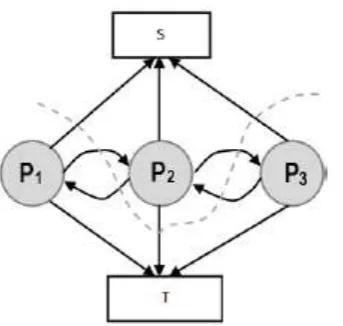
was shown that it is possible to _nd the global optimum of functions of this type using the graph-cut method. In

the graph-cut method, the MRF energy function is converted to a directional graph and the minimum s-t cut gives the desired segmenta- tion. A graph G D hV; Ei with two terminal nodes s and t representing the scar and healthy segmentation labels. The graph has a set of nodes V for every voxel in the image and E is the set of edges connecting these nodes (see Fig. 3). There are edges connecting every voxel to the two terminal nodes

International Journal of Advanced Technology in Engineering and Science www.ijates.com

Volume No 03, Special Issue No. 01, March 2015 ISSN (online): 2348 – 7550

1083 |

P a g e

Fig 3

image containing only 3 voxels.

The total cost of an s-t cut is equivalent to the sum of the edge weights the cut passes through. Fig. 3 graph of an image with only 3 voxels computes a possible segmentation. Note how the t-links are assigned a value based on the affinity of the node to the particular class label. In a similar way, the n-links represent affinity for neighbouring voxels, holding nodes with similar intensities together and resisting to a cut passing through them

resulting in a labeling of neighbouring voxels into two separate tissue classes.

III. EXPERIMENTS

The algorithm was evaluated on both numerical phantom andreal patient MRI datasets as described below.

3.1 Numerical Phantom Data

In the rest of the paper, the true location of scar is referred to as the ground-truth for scar. The extent of scarring

during ablation is non-deterministic and there is also confounding pre-ablation fibrosis. Therefore, identifying

locations where ablations were made is not sufficient to be a surrogate for the ground truth for scar. Moreover,

there is a high degree of inter- and intra-observer variability in manual segmentations of scar. These make

evaluating algorithms more difficult and challenging. To overcome these issues, numerical phantoms were

employed to extensively validate the algorithm.

3.1.1 Phantom Construction

The phantom was constructed in a four step process. The result of some steps is shown in Fig. 4. In the _rst step

the LA geometry was extracted from a typical patient dataset. In the second step, a 2.5 mm wall was constructed

around the LA. This represented LA wall. In a third step, regions were manually drawn within the constructed

LA wall; these regions represented scar. In the final fourth step, intensities were sampled randomly from

pre-determined distributions. These distributions belong to LA wall and blood-pool, and are measured and obtained

from real MRI data. This ensured likeness of the phantoms to real MRI. Scar was filled with intensities from

International Journal of Advanced Technology in Engineering and Science www.ijates.com

Volume No 03, Special Issue No. 01, March 2015 ISSN (online): 2348 – 7550

1084 |

P a g e

experiments that follow. It is important to simulate partial voluming, anisotropic voxel sizes and noise in the

phantoms. An anisotropic blur was applied with a kernel size of 2 mm in the through-plane direction and 1 mm

in the in-plane direction. Gaussian white noise (_ D 0; _ D 1) was added to the image.

Fig 4

morphological dilation; scar (SC) drawn manually. (b) Assignment of intensity levels drawn randomly

from pre-defined Gaussian distributions, with separate distributions for each tissue class. (c) In-plane and

through-plane blurring followed by the addition of Gaussian white noise. Abbreviations: L - left side, R -

right side.

3.1.2 Phantom Experiments

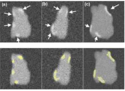
Numerical phantoms were generated by varying the SC-BP contrast ratio between 1.0 to 3.0. Some instances of

these phantoms can be seen in Fig. 5. This evaluated the algorithm's performance on scar with varying contrast

in relation to blood pool. The noise in the phantoms was maintained at signal-to-noise (SNR) of 9.0. This was

the average SNR observed on a cohort of clinical datasets. Training (n D 50) and testing (n D 50) data sets were generated accordingly. To make training as realistic as possible, it was separately trained on SC-BP ratios:

1.5_1.8 and 1.8_2.1. The algorithm was compared to ground-truth using the Dice overlap co-efficient [37].

FIGURE 5

.

Single slices through three different phantoms with numerically generated scars

indicated by the arrows (Top row). BP contrast is varied keeping SNR constant at 9.0.

SC-BP: (a) 1.4, (b) 1.6 and (c) 1.8. The segmentations from the algorithm are also shown (Bottom

row). In a separate experiment, the SNR was varied from 4 to 16 along with the SC-BP contrast

International Journal of Advanced Technology in Engineering and Science www.ijates.com

Volume No 03, Special Issue No. 01, March 2015 ISSN (online): 2348 – 7550

1085 |

P a g e

the above experiments on scar enhancement and noise variation, the performance of the

algorithm and fixed models (FWHM and n-SD) were compared on the same dataset. Five

separate phantoms were used from which 200 different scarred regions were identified and

their SC-BP contrast ratio noted. The accuracy with each method segmented each of the 200

regions was measured with Dice and reported.

3.1.3 Clinical Data

A total of 15 clinical human datasets were available. In these set of experiments, segmentations from the

algorithm were compared to the combined manual segmentations of three observers. In addition to this, the

algorithm was also compared to fixed models: FWHM and n-SD methods. Training for the algorithm was accomplished using the leave-one-out principle, where 14/15 datasets were used for training and 1/15 used for

testing. In the test scan, segmentation performance was measured both locally and globally for the image. For

local comparison, performance on individual sections of scar was measured (a total of 155 regions were

considered) and for a global comparison, total scar volume was measured. The pre-processing (left atrium

geometry extraction and registration) was the same for each approach. Three experienced observers manually

segmented scars in each DE-MRI scan. They were combined to generate a consensus segmentation or pseudo

-ground truth for each scan. This is necessary in order to consolidate inter-observer variability’s. Segmentations

were combined using the STAPLE algorithm described in [38]. For each voxel, a probability estimate for the

scar label could be computed. The STAPLE ground-truth was then be obtained by considering voxels to be scar

if their probability is greater than 0.7, or 70%. This is a reasonable threshold capable of generating a strong

consensus segmentation (In [38] the authors chose a lower consensus at 50%). To explore this threshold further,

an experiment was performed by varying the threshold. Segmentations were available from five experienced

observers on a random subset of the clinical datasets. The segmentations were combined using STAPLE and

three thresholds were considered:1) < 20%, 2) _ 20% and 3) _ 70%. This generated different consensus

segmentations with varying degrees of consensus against which the algorithm's performance was measured.

Finally, to further explore whether better training of the algorithm leads to better segmentations and thus better

performance, different instances of the algorithm are evaluated by incrementing the number of training set.

It is important to note that segmentations from the proposed algorithm were obtained without any user interact-

tion necessary at any step of the algorithm. The most com putationally demanding step was that of graph-cuts.

On images of the resolution described above, there are typically 50 000_100 000 nodes that require processing.

However, each step of the iterative process took less than a minute. The total running time of the proposed

approach is less than a minute on a 2.5 GHz PC.

3.2 Evaluation Metrics

To our experience, there is no single metric which works best for comparing segmentation overlaps. We chose

two different metrics to quantify segmentation overlap.

3.2.1 Regional Overlap

International Journal of Advanced Technology in Engineering and Science www.ijates.com

Volume No 03, Special Issue No. 01, March 2015 ISSN (online): 2348 – 7550

1086 |

P a g e

3.2.1

Sensitivity And Specificity

The proportion of true positives and true negatives in the detection process was analyzed by means of Receiver

Operating Characteristic (ROC) curves where possible.

3.2.3 Total Scar Volume

Segmentations were also compared by measuring the total scar volume. This is mostly how scar is quantified

and inter preted in clinical studies [39] and also serves as an important indicator for the total scar burden on the

atrium.

IV. RESULTS

4.1 Numerical Phantoms

4.1.1 Scar Contrast

Fig. 6 show results from testing the algorithm on phantoms generated by varying the SC-BP contrast.

Segmentation overlap with known true location of scarwas measured using Dice.The algorithm performs well

within its training range with median Dice _ 80 in both ranges: 1:5 _ SC-BP _ 1:8 [Fig. 6(a)] and 1:8 _ SC-BP _

2:2 [Fig. 6(b)]. Outside its training area, the algorithm showed that it is able to adapt to excellent SC-BP contrast

(_ 2:2) and good segmentations were achieved. Values of SC-BP explored in this experiment included realistic

DE-MRI values but SC-BP _ 3:0 is very difficult to achieve in practice. To summarise, this experiment

evaluated the algorithm across a wide dynamic SC-BP con- trast range and the algorithm's approximation of

ground truth was found to be good.

4.1.2 Noise Variation

Fig. 7 show results from testing the algorithm on phantoms generated by varying SNR. The SNR is varied

between 4 and 16. The algorithm is trained on datasets generated with SC-BP ranging between 1:8 _ SC-BP _

2:1. Results show that SC-BP dictates over SNR for achieving good segmentations. Note segmentations are poor

with SC-BP D 1:2 when SNR D 4 and with SNR D 16. But this is improved when SC-BP _ 1:8 demonstrating

that the algorithm is robust to noise. SNR in actual DE-MRI is typically around 9.0 and the

International Journal of Advanced Technology in Engineering and Science www.ijates.com

Volume No 03, Special Issue No. 01, March 2015 ISSN (online): 2348 – 7550

1087 |

P a g e

Fig 6

.

Performance of algorithm on numerical phantoms with increasing SC-BP contrast and

SNR fixed at 9.0. Each graph is an instance of the algorithm: (a) trained on 1.5 to 1.8, and (b)

trained on 1.8 to 2.1. The trend-lines show the median. Boxes in the plot indicate the 9th, 25th,

50th, 75th and 91st percentiles

Fig 7. Performance of algorithm on numerical phantoms with varying SNR. The SNR is varied

between 4 to 16. The median Dice segmentation overlap is plotted for the trend line shown.

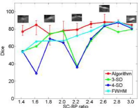
4.1.3 Comparison With Fixed Models

Fig. 8 show how the algorithm and fixed models per- formed on the same datasets. A total of 200 scarred

International Journal of Advanced Technology in Engineering and Science www.ijates.com

Volume No 03, Special Issue No. 01, March 2015 ISSN (online): 2348 – 7550

1088 |

P a g e

and the plots in Fig. 8 show the segmentation accuracy trend. Fixed models 3,4,6-SD generated better

segmentations than FWHM when scar contrast is between 1.2 to 2.2. However, FWHM improved substantially

with higher scar contrast (SC-BP > 2:2 in Fig. 8), which is when the 50 percent cut-off was more reasonable.

Overall, as illustrated in Fig. 8, the algorithm maintained good accuracy when compared to fixed models in

numerical phantoms.

Fig 8.

Comparing performance of algorithm with fixed models on numerical phantoms. Fixed

models namely 3-SD, 4-SD, 6-SD and FWHM were evaluated. The trend-lines show the median

Dice computed from 200 different scarred regions obtained from 5 separate phantoms

The failure of FWHM revealed in this experiment is further illustrated in Fig. 9 (see columns 1 and 2). When the

contrast in scar is not high, 50 percent of maximal signal as considered in FWHM, is not optimal and leaks in

segmentation are inevitable [Fig. 9 (row 3)].

Fig 9. Instances where 50% cut-off in FWHM is not optimal. First row: Original images of

phantom with variable scar contrast. Second row: Algorithm's segmentation. Third row:

International Journal of Advanced Technology in Engineering and Science www.ijates.com

Volume No 03, Special Issue No. 01, March 2015 ISSN (online): 2348 – 7550

1089 |

P a g e

4.2 Clinical Data

4.2.1 Comparison With Fixed Models Using Overlap Metric

In the clinical datasets, performance of algorithm and fixed models were tested by measuring overlap with

pseudo ground-truth (STAPLE) and comparing segmentation outputs in terms of scar volumes. For assessing

performance based on overlap, each method was tested on individual SC-BP contrast levels: 1.0, 1.4, 1.8, 2.2,

2.6 and 3.0. This was possible by sampling 155 individual scarred regions from the clinical scans, measuring

their SC-BP contrast ratio and testing how well each method segmented it. Results are given in Fig. 10.

FIGURE 10

.

Comparing performance of fixed models with algorithm on patient scans. The

performance over a total of 155 scarred regions are shown here. The trend-lines show the

median. Five example snapshots of scar are also given to illustrate SC-BP contrast levels. Note

SC-BP ratios analysed range from 1.4 to 3.0. Fixed models perform less accurately than the

algorithm when SC-BP is less than 2.5. At excellent and rarely attainable SC-BP levels (>> 2:5),

this trend changes and all models perform equally well. FWHM and the algorithm perform

consistently across the entire SC-BP range used in this experiment, with 3- and 4-SD models

outputting less accurate segmentations on scar at certain SC-BP contrast levels (1.6,2.2). This is

because scar is not adequately segmented by 3- or4-SD due to non-overlapping intensities

between model and actual. These results highlight that the algorithm performs consistently on

actual DE-MRI and across realistic SC-BP levels. Performance of fixed models is found to be

variable

.

4.2.2 Comparison with Fixed Models Using Quantified Volume

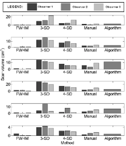
Assessment of performance using total scar volume reported by each method is important as this is mostly how

scar is quantified and interpreted for clinical studies. Results obtained from scar volume quantified by each run

of method are given in Fig. 11 for six clinical datasets. Each method was run three separate times with inputs

International Journal of Advanced Technology in Engineering and Science www.ijates.com

Volume No 03, Special Issue No. 01, March 2015 ISSN (online): 2348 – 7550

1090 |

P a g e

method was compared to the volume reported by three independent experienced observers (see Manual method

in Fig. 11).

Fig 11. Assessment of inter-observer variation in fixed models, manual segmentation and

algorithm. Six clinical cases are illustrated here

The algorithm correlated well with manual scar volumes. All three runs of the algorithm produced the same

result as depicted by the single bar in Fig. 11. All other methods showed vari- ations in the quantified volume.

This variation was primarily due to observer variability in selecting normal or hyper-enhanced tissue required

for _xed models. This high- lights that a standardized quantification for scar using a fixed model approach

(FWHM and SD) can be difficult to achieve.

4.2.3 Qualitative Comparison On De-Mri Scans

Segmentation quality was assessed by overlaying region contours over the original DE-MRI slices. It was

generally observed that in images with excellent SC-BP contrast, contours followed scar boundaries accurately

in both algorithm and fixed models. Fixed models 3 and 6-SD were less accurate. An example is shown in Fig.

15 where segmentations similar to the consensus segmentation [Fig. 15(b)] could be obtained. Fixed models

showed poor correlation when the SC-BP contrast is not sufficiently high. An example is shown in Fig. 16

where FWHM and the algorithm fared well with the algorithm providing a better approximation to the

consensus segmentation. Fixed models 3 and 6-SD have gross errors in their segmentations due to a large

overlap of intensities between their scar model and actual healthy tissue. Such segmentations are not usable for

International Journal of Advanced Technology in Engineering and Science www.ijates.com

Volume No 03, Special Issue No. 01, March 2015 ISSN (online): 2348 – 7550

1091 |

P a g e

4.2.4 Analyzing Algorithm Performance By Varying Consensus Levels Of Pseudo Ground

Truth

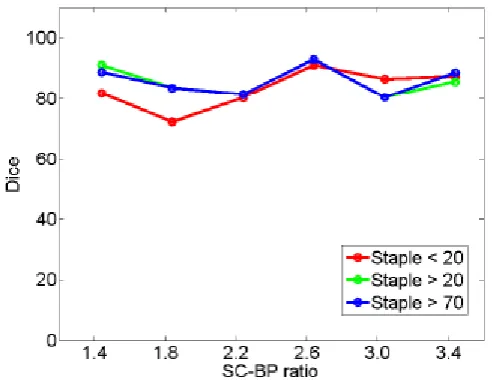
The algorithm's performance on a subset of clinical datasets was evaluated by varying the STAPLE threshold

and thus the level or strength of the consensus segmentation. Results are plotted in Fig. 12 showing

segmentation overlap on three consensus levels. There was a small difference in the algorithm's performance

noted when BP contrast levels were low. With higher BP the performance was nearly similar. When

SC-BP contrast is poor, the consensus or agreement between observers can be low. By lowering the acceptable

consensus threshold (to 20%), dubious pixels are included in the ground truth where 2/10 observers would agree

that it is scar. As the algorithm generally selects pixels which have close affinity to its models and priors,

dubious pixels are omitted by the algorithm. There is a decrease in performance when segmentations with low

consensus are presented.

Fig 12

.

Performance trends of the algorithm on STAPLE consensus ground truths. Each curve

represents performance on consensus segmentations, with consensus varied from 20% (weak) to

70% (strong).

4.2.5 Analyzing Algorithm Performance By Varying Strength Of The Training Set

The algorithm's training set was incrementally increased and its segmentation overlap performance was noted.

There was little notable difference in the performance. Results are plotted in Fig. 13. Training had an impact on

performance only when the training set and test set had similar SC-BP contrast levels. If these vastly differ,

initial iterations of the algorithm generate poor segmentations and these progressively become better in later

iterations when the scar intensity model is continuously adapted with feedback from previous iterations (refer to

'adapting training step' in Fig. 2).

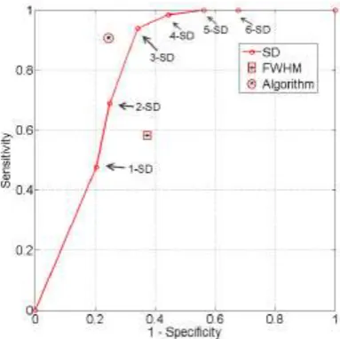
4.2.6 Roc Analysis

The true positive and true negatives rates were analyzed by looking at sensitivity and specifity of the algorithm

and the fixed-models. A ROC curve between sensitivity and specificity was only plotted, where each point on

International Journal of Advanced Technology in Engineering and Science www.ijates.com

Volume No 03, Special Issue No. 01, March 2015 ISSN (online): 2348 – 7550

1092 |

P a g e

where the decision threshold was varied between n D 1 to n D 6. Since both the algorithm and FWHM do not

require a decision threshold for obtaining segmentations, their overall sensitivity and specificity on all datasets

was plotted

Fig 13.

Performance trends of the algorithm by increasing the training set. Each curve

represents an instance of the algorithm trained on n D 9; 7; 5 datasets

.

Fig 14.

ROC analysis of the algorithm, FWHM and n-SD method. The ROC curve is only

plotted for the n-SD method and the overall sensitivity and specificity is plotted for the

parameter-less proposed algorithm and FWHM.

The n-SD fixed model approach has low specificity for n D 1; 2; 3 and increasingly mislabelled healthy tissues as scar. However, its higher sensitivity indicated that scar tissues are mostly labelled correctly. This reversed

International Journal of Advanced Technology in Engineering and Science www.ijates.com

Volume No 03, Special Issue No. 01, March 2015 ISSN (online): 2348 – 7550

1093 |

P a g e

individual regions where it was shown that its 50% cut-off is too low for scar with low SC-BP, but more suitable

for high SC-BP ratios.

FIGURE 15.Segmentations on clinical scans I: (a) original scan, (b) consensus STAPLE segmentation, (c)

Algorithm, (d) FWHM, (e) 3-SD, (f) 6-SD. Arrows show enhancement. This scan has excellent SC-BP

contrast and all methods except 3-SD and 6-SD demonstrate good accuracy. Abbreviations: AO - Aorta,

LA - Left atrium, R - Right side, L - left side.

Fig 16.

Segmentations on clinical scans II: (a) original scan, (b) consensus STAPLE

International Journal of Advanced Technology in Engineering and Science www.ijates.com

Volume No 03, Special Issue No. 01, March 2015 ISSN (online): 2348 – 7550

1094 |

P a g e

V. DISCUSSION

In this work a segmentation algorithm was investigated for fast quantification of fibrosis in DE-MRI scans. The

proposed algorithm offers the following advantages: 1) Segments fibrosis without requiring a manual outline of

remote or healthy myocardium. This is beneficial since remote myocardium tends to have low SNR and manual

selection suffers from\ high observer variability. 2) The algorithm does not routinely generate false positives as

was observed in existing fixed model methods: FWHM and n-SD. 3) The algorithm is developed particularly for

left atrial fibrosis segmentation and all present approaches were developed for ventricle scans. 4) Analysis of

DE-MRI scans was shortened to an average of 30 seconds when compared to existing semi-automatic

approaches requiring 2 minutes per scan on average. The algorithm along with existing approaches was tested

on both numerical phantoms and clinical datasets. Numerical phantoms provided with a wide dynamic range of

variation.

VI. CONCLUSION

DE-MRI is becoming a preferred method for non-invasive imaging of myocardial scar. The amount of scar

predicts whether a patient will respond to RFCA procedures. Thus accurately quantifying scar is important and

has implications in patient selection for RFCA. Currently, SD and FWHM fixed thresholding models are

frequently utilized clinically to quantify scar due to their simplicity. Present literature has only evaluated these

methods using global image measures and thus their deficiencies could not be noted. In this work, there are two

important contributions: 1) SD and FWHM fixed models are evaluated on individual regions of scar and thus

various scar contrast ratios are examined to show they fail when some contrast levels do not suit the selected

threshold in SD or 50% cut-off in FWHM. This is further confirmed and validated in numerical phantoms. 2)

the proposed algorithm has the potential to standardize quantification of scar from routine clinical scans; it

requires no threshold selection and is shown to be more sensitive and specific than SD and FWHM in scar

detection. Accurate and standardized quantification will allow appropriate selection of patient candidates for

RFCA. This could considerably reduce the recurrence rates, procedure risk and high financial burden associated

with unsuccessful RFCA treatment. Patients not deemed appropriate for RFCA based on their scar assessment

could be treated far less invasively using drug therapy. A standardized quantification of scar in DE-MRI is thus

necessary.

ACKNOWLEDGMENT

Dandu Nasreen Sulthana born in kalakada, chittoor dist, A.P, India in 1992. He received B.Tech Degree in

(DECS) from Annamacharya Institute of Technology & Sciences, Rajampet, A.P., India.

S. Asif Hussain

JNT University,Anantapur, India. He is an associative professor in the Department of ECE at the

Annamacharya Institute of Technology & Sciences (an Autonomous Institute), in Rajampet, Andhra Pradesh.

International Journal of Advanced Technology in Engineering and Science www.ijates.com

Volume No 03, Special Issue No. 01, March 2015 ISSN (online): 2348 – 7550

1095 |

P a g e

BMESI,IACSIT, IAENG etc. He has presented many research papers at national and international conferences.

REFERENCES

[1] A. Go et al., ``Prevalence of diagnosed atrial fibrillation in adults,'' J. Amer. Med. Assoc., vol. 285, no. 18, pp. 2370_2375, 2001.

[2] J. P. Piccini et al., ``Incidence and prevalence of atrial fibrillation and associated mortality among medicare beneficiaries: 1993_2007,'' Circulat., Cardiovascular Qual. Outcomes, vol. 5, no. 1, pp. 85_93, 2012. [3] M. Haissaguerre et al., ``Spontaneous initiation of atrial fibrillation by ectopic beats originating in the

pulmonary veins,'' New England J. Med., vol. 339, no. 10, pp. 659_666, 1998.

[4] C. Pappone et al., ``Circumferential radiofrequency ablation of pulmonary vein ostia: A new anatomic approach for curing atrial fibrillation,'' Circulation, vol. 102, no. 21, pp. 2619_2628, 2000.

[5] H. Oral et al., ``Circumferential pulmonary-vein ablation for chronic atrial fibrillation,'' New England J. Med., vol. 354, no. 9, pp. 934_41, 2006.