Temporal and spatial variations in ionospheric electron density proﬁles over South Africa during strong magnetic storms

(1)

Nat. Hazards Earth Syst. Sci., 13, 375–384, 2013 www.nat-hazards-earth-syst-sci.net/13/375/2013/ doi:10.5194/nhess-13-375-2013

EGU Journal Logos (RGB)

Advances in

Geosciences

Open Access

Natural Hazards

and Earth System

Sciences

Open Access

Annales

Geophysicae

Open Access

Nonlinear Processes

in Geophysics

Open Access

Atmospheric

Chemistry

and Physics

Open Access

Atmospheric

Chemistry

and Physics

Open Access

Discussions

Atmospheric

Measurement

Techniques

Open Access

Atmospheric

Measurement

Techniques

Open Access

Discussions

Biogeosciences

Open Access Open Access

Biogeosciences

Discussions

Climate

of the Past

Climate

of the Past

Discussions

Earth System

Dynamics

Earth System

Dynamics

Discussions

Geoscientific

Instrumentation

Methods and

Data Systems

Open Access

_{Geoscientific}

Instrumentation

Methods and

Data Systems

Open Access

Discussions

Geoscientific

Model Development

Geoscientific

Model Development

Discussions

Hydrology and

Earth System

Sciences

Open Access

Hydrology and

Earth System

Sciences

Open Access

Discussions

Ocean Science

Discussions

Solid Earth

Discussions

The Cryosphere

Natural Hazards

and Earth System

Sciences

Open Access

Discussions

Temporal and spatial variations in ionospheric electron density

profiles over South Africa during strong magnetic storms

Y. B. Yao1,2, P. Chen1,3, S. Zhang1, and J. J. Chen1

1_{School of Geodesy and Geomatics, Wuhan University, Wuhan 430079, China}

2_{Key Laboratory of Geospace Environment and Geodesy, Ministry of Education, Wuhan University, Wuhan 430079, China} 3_{College of Geomatics, Xi’an University of Science and Technology, Xi’an 710054, China}

Correspondence to: Y. B. Yao ([email protected])

Received: 14 October 2012 – Published in Nat. Hazards Earth Syst. Sci. Discuss.: – Revised: 9 January 2013 – Accepted: 10 January 2013 – Published: 15 February 2013

Abstract. Observations from the South African TrigNet global navigation satellite system (GNSS) and vertical total electron content (VTEC) data from the Jason-1 satellite were used to analyze the variations in ionospheric electron density profiles over South Africa before and after the severe geo-magnetic storms on 15 May 2005. Computerized ionospheric tomography (CIT) was used to inverse the 3-D structure of ionospheric electron density and its response to the magnetic storms. Inversion results showed that electron density signif-icantly increased at 10:00 UT, 15 May compared with that at the same period on 14 May. Positive ionospheric storms were observed in the inversion region during the magnetic storms. Jason-1 data show that the VTEC observed on de-scending orbits on 15 May significantly increased, whereas that on ascending orbits only minimally changed. This find-ing is identical to the CIT result.

1 Introduction

A geomagnetic storm is a complex process that originates from solar wind and the magnetosphere. It is one of the most important phenomena related to solar wind and so-lar energetic particles. Geomagnetic storms can cause severe global ionospheric disturbance and affect the neutral atmo-sphere, including the troposphere and middle atmosphere. Accompanied by magnetic storms, ionospheric total elec-tron content (TEC), ionospheric F2 layer critical frequency, and other ionospheric parameters exhibit drastic changes that can last for several hours to a few days. Appleton and In-gram (1935) first defined strong ionospheric disturbances

during geomagnetic storms as ionospheric storms. Numerous scholars have conducted research on such storms, but defini-tive findings have yet to be obtained. Studies on ionospheric storms remain a challenge for ionospheric researchers (Zhao, 2006).

Considerable research has revealed the fundamental laws of ionospheric storms. Generally, ionospheric storms at high latitudes are mainly negative-phase storms (i.e. the iono-spheric electron density is significantly lower than the av-erage ionospheric state), whereas those occurring at low latitudes are primarily positive-phase storms (i.e. the iono-spheric electron density significantly greater than average ionospheric state). Whether a specific ionospheric storm is a positive- or negative-phase storm is determined by the local time at which the main phase of the storm occurs. At mid-dle latitudes, if the main phase occurs in the morning, then the ionospheric storm is classified as of positive-phase type. If the main phase occurs in the afternoon, the ionospheric storm is categorized as a weak positive-phase storm; an in-tense negative-phase storm occurs the following day. The oc-currence of the main storm phase at nighttime typically gen-erates a negative-phase storm the next day (Balan and Rao, 1990). Kelley et al. (2004) suggested that daytime eastward prompt penetration electric field (PPEF) that produces nega-tive storms inNmaxand TEC at equatorial latitudes through

enhanced plasma fountain (Balan et al., 2009) could also be the main driver of the positive storms at higher latitudes. However, modeling studies later revealed that the PPEF alone is unlikely to produce the positive storms and equatorward neutral winds alone (Balan et al., 2009) or together with PPEF (Lin et al., 2005; Lu et al., 2012) can produce the

(2)

376 Y. B. Yao et al.: Temporal and spatial variations in ionospheric electron density profiles

positive storms. The physical mechanisms of why the east-ward PPEF is unlikely to produce the positive storms, and how the neutral winds produce the positive storms have been reported recently (Balan et al., 2010, 2011).

Early ionospheric storm research was based primarily on single-station observations, later gradually developing into studies that feature local area observations from multiple sta-tions and global station networks. Paul et al. (1977) used observations from 35 ionospheric stations and seven geo-magnetic stations in the Asia-Pacific region to investigate the ionospheric storm that occurred on 4–5 August 1972. The results showed that electron density sharply increased after the initial phase of the magnetic storm, and the peak occurred between geomagnetic latitudes 20◦ and 45◦. Us-ing observations from 40 ionosonde stations and TEC data from 12 GPS stations, Yeh et al. (1994) investigated the global ionospheric response during the strong geomagnetic storm in October 1989. Szuszczewicz et al. (1998) used ob-servations from 53 global ionosonde stations to investigate the ionospheric response during three strong geomagnetic storms in September 1989. The results showed that the hmF2 and NmF2 were related to the local time, latitude, and time of occurrence of geomagnetic storms. Mannucci et al. (2005) studied the ionospheric changes during the “Halloween” su-per magnetic storm in 29–30 October 2003. The dayside ionospheric TEC on 29 and 30 October increased by 40 % and 250 %, respectively. The significant ionospheric change may have been caused by the eastward equatorial electric field during the storm. Essex et al. (1981) used data from 18 global stations to study the ionospheric response after the geomagnetic storm on 17 June 1972, and compared it with the ionospheric response after the magnetic storm on 17 De-cember 1971.

A number of studies focused on the statistical properties of ionospheric storms. Balan et al. (2010) used TEC andNmax

data to investigate the time of occurrence and strength of the ionospheric response at low latitudes after the 60 magnetic storms that occurred from 1968 to 1972. Mendillo and Nar-vaez (2009, 2010) usedNmaxdata to study the ionospheric

changes after the 206 magnetic storms that occurred from 1964 to 1976. Lekshmi et al. (2011) used data from two ionosonde stations in Japan and the United States to de-termine the ionospheric response characteristics of the 584 magnetic storms of two solar cycles that occurred from 1985 to 2005. Some scholars used models to simulate the gener-ation of ionospheric storms and study the physical mecha-nisms of such storms (Burns et al., 1995; Fuller-Rowell et al., 1994; Lin et al., 2005; Lu et al., 2008; Richmond and Matsushita, 1975).

The late 1970s saw the rise of GNSS, which improved ionospheric sounding technology. Since then, ionospheric research has gone through rapid development. GNSS rep-resents a new technology that obtains accurate TEC val-ues from satellites and receivers, and continuously moni-tors ionospheric changes over a wide geographical range.

GNSS-based computerized ionospheric tomography (CIT) technology was then gradually developed to aid the under-standing of the full range of temporal and spatial distribu-tions of ionospheric electron density. New CIT technology enables the 3-D and 4-D reconstruction of the spatial struc-ture of the ionosphere. Using GPS data from Chinese GNSS stations and CIT, Wen et al. (2007) studied the temporal and spatial changes in ionospheric electron density profiles over China during the magnetic storm on 18 and 21 Au-gust 2003. Thampi et al. (2009) used CIT to investigate sum-mer night ionospheric anomalies that occur at middle lat-itudes. Yao et al. (2012a) used CIT technology to inverse the 3-D variations in ionospheric electron density before the JapanMw=9.0 earthquake on 11 March 2011. The authors

excluded the effects of magnetic storms in their study. The results showed that significant positive anomalies in the iono-spheric electron density profile could be detected before the earthquake. Yao et al. (2012b) investigate the unusual iono-spheric total electron content (TEC) variations which oc-curred before the globalM=7.0+earthquakes in 2010, and confirmed that the earthquake-related ionospheric anomalies discussed in the paper occurred 0–2 days before the associ-ated earthquakes and in the afternoon to sunset. Yizengaw et al. (2005) used ground-based and satellite data to investigate the ionospheric response in the Southern Hemisphere during the magnetic storms on 31 March 2001. The authors used the chain of GPS receiver stations near 150◦E to inverse the ionospheric electron density variations at 150◦E longitude during the storms. Mai and Kiang (2009) used CIT technol-ogy to inverse the ionospheric anomalies that occurred after the 2004 Sumatra tsunami.

To compensate for the lack of GNSS tracking stations in marine areas, researchers used altimetry satellite data to di-rectly access TEC trends over the global ocean (Dumont et al., 2009; Fu et al., 1994; Jee et al., 2004).

In the current work, data derived by GNSS CIT technology and the Jason-1 ocean altimetry satellite were used to ana-lyze the spatial and temporal variations in ionospheric elec-tron density before and after the severe magnetic storm on 15 May 2005. The response of ionospheric electron density to magnetic storms is also discussed.

1.1 Geomagnetic environment in solar and interplanetary space

Solar activity was intense after 10 May 2005. From 10 to 13 May, sixM-class flares were observed, among which an

M=8.0 flare occurred on 13 May at 16:13 UT to 17:28 UT. The giant storm on 15 May was directly caused by the coronal mass ejections produced by theM=8.0 flare. Fig-ure 1 shows the satellite records of interplanetary mag-netic field strength, the Bz component of the interplane-tary magnetic field, and solar wind speed, as well as the Kp, Dst, and AE indices recorded by geomagnetic stations on Earth. An intense magnetic storm occurred on 15 May,

(3)

Y. B. Yao et al.: Temporal and spatial variations in ionospheric electron density profiles 377

and the Dst variation showed that this storm was a sudden-commencement magnetic storm. Solar wind speed drasti-cally increased at 00:00 UT on 15 May. At 10:00 UT, solar wind speed exceeded 900 km s−1, twice the speed of that occurring at the same period the day before. The Bz com-ponent of the interplanetary magnetic field reached−40 nT at around 06:00 UT on 15 May. The signature of the subse-quent Bz component rapidly changed to north and continued on this course for a while, then shifted between the north and south directions. The dramatic changes in the interplan-etary magnetic field triggered a magnetic storm with a sud-den commencement time at 06:12 UT. Dst rapidly increased from 4 nT to 45 nT at 03:00 UT on 15 May, then quickly de-creased at 06:00 UT. The main phase of the storm occurred at 08:00 UT, when the Dst index was−263 nT and the Kp in-dex was 8+. Simultaneously, the AE index rapidly increased, representing the considerable solar energy injected into the ionosphere. The Dst index then gradually increased, and the magnetic storms reached the recovery phase. On 20 May, the Dst index returned to the normal state before the magnetic storm occurred.

1.2 Selection and processing of GNSS observation data

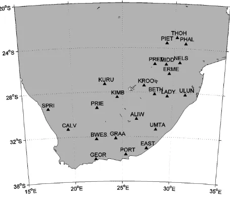
To study the temporal and spatial distributions of the iono-spheric disturbances at low-latitude regions in the Southern Hemisphere during the magnetic storm, we used data from the South African TrigNet network data to inverse the 3-D distribution of local ionospheric electron density before and after the magnetic storm on 15 May 2005. We then ana-lyzed the temporal and spatial variations in ionospheric elec-tron density in the abnormal space environment. TrigNet is a continuously operating GNSS network that covers South Africa; the distance between the base stations of TrigNet is 200 km to 300 km. In 2005, TrigNet was a network compris-ing 23 continuous trackcompris-ing stations. The distribution of these tracking stations is shown in Fig. 2. We inverted the vari-ations in ionospheric electron density during the magnetic storm using dual-frequency GPS observation data from 23 base stations from 14 to 15 May 2005. The time interval of the dual-frequency GPS observation data is 30 s.

When CIT technology is used to inverse the temporal and spatial variations in ionospheric electron density in anoma-lous space environments, the first step is to preprocess orig-inal observation data. We used the Turbo Edit method (Ble-witt, 1990) to detect and repair the errors and cycle slips in the GPS observation data. Then, the geometry-free pseudor-ange and carrier phase were used to come up with basic ob-servations. Finally, the STEC was calculated along the signal propagation path between each satellite and receiver. In this paper, the cut-off angle used was 10◦. In accordance with the influence of system hardware delays, we employed a typical approach, in which we constructed a single-layer ionospheric model, resolved satellite hardware delays, and used model parameters to solve receiver hardware delays as unknown

the interplanetary magnetic field, and solar wind speed, as well as the Kp, Dst, and AE indices

recorded by geomagnetic stations on Earth. An intense magnetic storm occurred on May 15, and

the Dst variation showed that this storm was a sudden-commencement magnetic storm. Solar wind

speed drastically increased at 00:00UT on May 15. At 10:00UT, solar wind speed exceeded

900 km/s, twice the speed of that occurring at the same period the day before. The Bz component

of the interplanetary magnetic field reached –40 nT at around 06:00UT on May 15. The signature

of the subsequent Bz component rapidly changed to north and continued on this course for a while,

then shifted between the north and south directions. The dramatic changes in the interplanetary

magnetic field triggered a magnetic storm with a sudden commencement time at 06:12UT. Dst

rapidly increased from 4 nT to 45 nT at 03:00UT on May 15, then quickly decreased at 06:00UT.

The main phase of the storm occurred at 08:00UT, when the Dst index was –263 nT and the Kp

index was 8+. Simultaneously, the AE index rapidly increased, representing the considerable solar

energy injected into the ionosphere. The Dst index

then gradually increased, and the magnetic

storms reached the recovery phase. On May 20, the Dst index returned to the normal state before

the magnetic storm occurred.

Figure 1 Solar and geomagnetic field parameters on 13 and 20 May 2005. The satellite records of interplanetary magnetic field Fig. 1. Solar and geomagnetic field parameters on 13 and

20 May 2005. The satellite records of interplanetary magnetic field strength, the Bz component of the interplanetary magnetic field, and solar wind speed, as well as the Kp, Dst, and AE indices recorded by geomagnetic stations are shown from top to bottom.

parameters. To derive precise results, we used two-day data to solve receiver hardware delays and then obtained the ab-solute STEC.

The ionospheric TEC is the line integral electron density on the signal propagation path. It is expressed as

TEC=

Z

l

N e(r, t )ds, (1)

whereN eis the electron density along the signal propagation pathl. GNSS-based ionospheric CIT uses a series of TECs along l to inverse the temporal and spatial distributions of ionospheric electron density. After discretizing Eq. (1) in the inversion process, we obtained

y=A·x+ε, (2)

(4)

strength, the Bz component of the interplanetary magnetic field, and solar wind speed, as well as the Kp, Dst, and AE indices

recorded by geomagnetic stations are shown from top to bottom.

3 Selection and processing of GNSS observation data

To study the temporal and spatial distributions of the ionospheric disturbances at low-latitude regions in the Southern Hemisphere during the magnetic storm, we used data from the South African TrigNet network data to inverse the 3D distribution of local ionospheric electron density before and after the magnetic storm on 15 May 2005. We then analyzed the temporal and spatial variations in ionospheric electron density in the abnormal space environment. TrigNet is a continuously operating GNSS network that covers South Africa; the distance between the base stations of TrigNet is 200 km to 300 km. In 2005, TrigNet was a network comprising 23 continuous tracking stations. The distribution of these tracking stations is shown in Figure 2. We inversed the variations in ionospheric electron density during the magnetic storm using dual-frequency GPS observation data from 23 base stations from 14 to 15 May 2005. The time interval of the dual-frequency GPS observation data is 30 seconds.

Figure 2 Distribution of TrigNet sites.

When CIT technology is used to inverse the temporal and spatial variations in ionospheric electron density in anomalous space environments, the first step is to preprocess original observation data. We used the Turbo Edit method (Blewitt, 1990) to detect and repair the errors and cycle slips in the GPS observation data. Then, the geometry-free pseudorange and carrier phase were used to come up with basic observations. Finally, the STEC was calculated along the signal propagation path between each satellite and receiver. In this paper, the cut-off angle used was 10°. In accordance with the influence of system hardware delays, we employed a typical approach, in which we constructed a single-layer ionospheric model, resolved satellite hardware delays, and used model parameters to solve receiver hardware delays as unknown parameters. To derive precise results, we used two-day data to solve receiver hardware delays and then obtained the absolute STEC.

The ionospheric TEC is the line integral electron density on the signal propagation path. It is

Fig. 2. Distribution of TrigNet sites.

GNSS signal propagation path;x represents the parameter vector constituted by the electron density of each pixel in the image of the ionosphere;ε is the noise vector of observa-tions.

Using Eq. (2) for ionospheric CIT indicates that coeffi-cient matrixAis a huge sparse matrix and usually rank de-ficient. The most common approach is to use an empirical model (e.g. the international reference ionosphere model) as the initial iteration value to obtain the electron density of the inversion region.

Given the non-negativity of electron density, we inverted it by the multiplicative algebraic reconstruction technique. The iterative formula can be written as

x_j(k+1)=x_j(k) yi ai, x(k)

! γ₀·_aij

A

, (3)

wherex(k)is the unknown parameter of thek-th iteration;ai

is thei-th row ofA;γ0denotes the relaxation factor of each

iteration, with 0< γ0<1.

To elucidate the features of the ionospheric disturbances during the magnetic storm, we used the GNSS observation data provided by the South African TrigNet. These data were also used to process the inversion. The inversion region is be-tween 16◦E to 32◦E and 22◦S to 36◦S at a height of 100 km to 1000 km. The size of the grid, which is 50 km high, is 2◦ both in latitude and longitude regions. Thus the ionosphere over South Africa is divided into 8, 7, and 19 grids along longitude, latitude, and height.

2 CIT results during storms

To study the temporal and spatial variations in ionospheric electron density before and after the magnetic storm, we

present the electron density distribution at different altitudes at 10:00 UT on 14–15 May 2005.

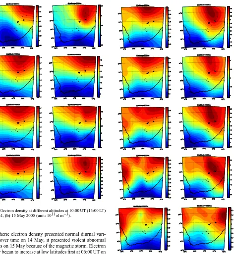
Figure 3 compares the ionospheric electron density at dif-ferent altitudes at 10:00 UT on 14 and 15 May. The elec-tron density at each altitude at 10:00 UT on 15 May signifi-cantly increased compared with the 14 May value, indicating that a positive-phase storm occurred in the ionosphere of the inversion region during the magnetic storm. The maximum electron density at each altitude at 10:00 UT on 15 May in-creased to 79.3 % on average compared with that on 14 May, during which the electron density at an altitude of 800 km increased to a maximum of 84.9 %. The minimum electron density increased to 30.7 %, similar to that at 800 km, which reached a maximum of 38.4 %. The peak electron density at an altitude of 300 km increased from 8.15×1011el m−3 to 1.36×1012el m−3_{. The electron density distributions during}

the two days both decreased with increasing altitude. Figure 4 shows a schematic of the temporal and spa-tial variations in electron density at an altitude of 350 km and a time interval of 2 h from 04:00 UT on 14 May to 20:00 UT on 15 May. Electron density significantly changed over time. For 40 h, electron density generally exhibited a high-to-low trend, significantly increased, and then gradually decreased. On 14 May, geomagnetic field activity was rela-tively calm, the electron density in the inversion region pre-sented normal diurnal variations over time, and the changes in normal ionospheric electron density were influenced pri-marily by the sun. The peak electron density was 1.75×

1011el m−3 at 04:00 UT, increased to 3.45×1011el m−3 at 06:00 UT, then gradually increased and reached a maxi-mum of 6.85×1011el m−3_{at 12:00 UT. The maximum}

elec-tron density lasted 2 h, then gradually decreased to 4.4×

1011el m−3 _{at 16:00 UT. It presented a minimum of 1.5}_×

1011el m−3 at 02:00 UT on 15 May before beginning to increase again. On 15 May, a strong magnetic storm oc-curred in the geomagnetic field, after which ionospheric electron density presented significantly abnormal changes. At a similar period on 14 May, the peak electron density at 06:00 UT increased by an insignificant rate of 15.9 %, i.e. 4×1011el m−3. At 08:00 UT, peak electron density in-creased to 7.3×1011 el m−3, a value 52 % higher than the increase on 14 May. It presented significantly positive ab-normal changes at 10:00 UT and reached 1.2×1012el m−3, a value 81.8 % higher than the increase on 14 May. At 12:00 UT, peak electron density continued to present positive anomalies at 31.4 % greater than those on 14 May. However, the ionospheric electron density in the inversion region pre-sented negative anomalies at almost 6 % less than those on 14 May. At 16:00 UT, peak electron density presented pos-itive anomalies at 37.5 % greater than those on 14 May. At 18:00 UT and 20:00 UT, the anomalies increased to 73.6 % and 22.2 %, respectively.

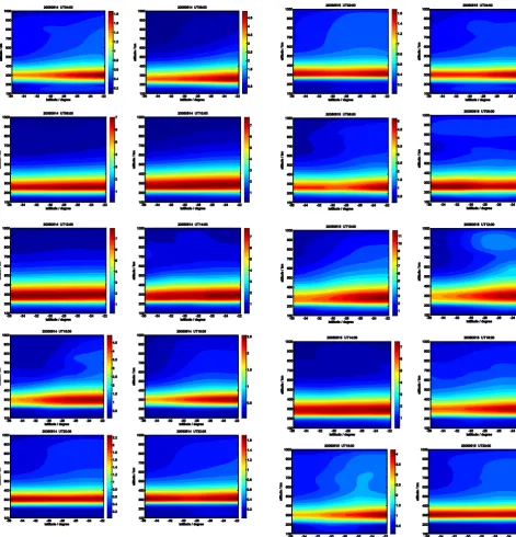
Figure 5 shows the temporal and spatial variations in elec-tron density on the 24◦E profile from 04:00 UT on 14 May to 20:00 UT on 15 May. Similar to Fig. 4, Fig. 5 shows that

(5)

during which the electron density at an altitude of 800 km increased to a maximum of 84.9%. The minimum electron density increased to 30.7%, similar to that at 800 km, which reached a

maximum of 38.4%. The peak electron density at an altitude of 300 km increased from 8.15×1011

el/m3 to 1.36×1012 el/m3. The electron density distributions during the two days both decreased with increasing altitude.

Fig. 3. Electron density at different altitudes at 10:00 UT (13:00 LT)

on (a) 14, (b) 15 May 2005 (unit: 1011el m−3).

ionospheric electron density presented normal diurnal vari-ations over time on 14 May; it presented violent abnormal changes on 15 May because of the magnetic storm. Electron density began to increase at low latitudes first at 06:00 UT on 14 May, then reached a maximum of 4.59×1011 el m−3at an altitude of 250 km between 22◦S and 24◦S. At 10:00 UT, the electron density at any altitude was roughly consistent with that at longitude 24◦_{E when peak electron density was} 8.04×1011 el m−3_{at an altitude of 300 km. At 14:00 UT, the}

ionospheric maximum electron density remained unchanged, but slightly declined to 7.68×1011el m−3at high latitudes. At 18:00 UT, the electron density significantly declined to 2.47×1011el m−3. The electron density further decreased to 1.6×1011el m−3from 22:00 UT on 14 May to 02:00 UT on 15 May. The ionosphere began presenting significantly abnormal changes with the magnetic storm at 06:00 UT on

Figure 3 Electron density at different altitudes at 10:00UT (13:00LT) on (a) 14, (b) 15 May, 2005 (unit: 1011_el/m3_).

Figure 4 shows a schematic of the temporal and spatial variations in electron density at an altitude of 350 km and a time interval of 2 hours from 04:00UT on May 14 to 20:00UT on 15May. Electron density significantly changed over time. For 40 hours, electron density generally exhibited a high-to-low trend, significantly increased, and then gradually decreased. On 14May, geomagnetic field activity was relatively calm, the electron density in the inversion region presented normal diurnal variations over time, and the changes in normal ionospheric electron density were influenced primarily by the sun. The peak electron density was 1.75×1011 el/m3at

04:00UT, increased to 3.45×1011

el/m3

at 06:00UT, then gradually increased and reached a

maximum of 6.85×1011el/m3at 12:00UT.The maximum electron density lasted 2 hours, then

gradually decreased to 4.4×1011el/m3at 16:00UT. It presented a minimum of 1.5×1011el/m3at

02:00UT on 15May before beginning to increase again.On 15May, a strong magnetic storm

occurred in the geomagnetic field, after which ionospheric electron density presented significantly abnormal changes. At a similar period on 14 May, the peak electron density at 06:00UT increased

by an insignificant rate of 15.9%, i.e., 4×1011el/m3. At 08:00UT, peak electron density increased

to 7.3×1011 el/m3, a value 52% higher than the increase on 14 May. It presented significantly

positive abnormal changes at 10:00UT and reached 1.2×1012

el/m3

, a value 81.8% higher than the increase on 14 May. At 12:00UT, peak electron density continued to present positive anomalies at 31.4% greater than those on 14 May. However, the ionospheric electron density in the inversion region presented negative anomalies at almost 6% less than those on 14 May. At 16:00UT, peak electron density presented positive anomalies at 37.5% greater than those on 14 May. At 18:00UT and 20:00UT, the anomalies increased to 73.6% and 22.2%, respectively.

Fig. 3. Continued.

15 May. The anomaly also increased with the continuous development of the magnetic storm. At 06:00 UT, the iono-spheric maximum electron density was 5×1011el m−3at an altitude of 260 km without significant anomalies compared with the same period on 14 May. At 10:00 UT, however, electron density significantly increased to 1.3×1012el m−3, which is 61.7 % higher than that on 14 May. This value is particularly significant between 22◦S and 30◦S. The results

(6)

380 Y. B. Yao et al.: Temporal and spatial variations in ionospheric electron density profiles Figure 3 Electron density at different altitudes at 10:00UT (13:00LT) on (a) 14, (b) 15 May, 2005 (unit: 1011_el/m3_).

Figure 4 shows a schematic of the temporal and spatial variations in electron density at an

altitude of 350 km and a time interval of 2 hours from 04:00UT on May 14 to 20:00UT on 15May. Electron density significantly changed over time. For 40 hours, electron density generally

exhibited a high-to-low trend, significantly increased, and then gradually decreased. On 14May, geomagnetic field activity was relatively calm, the electron density in the inversion region

presented normal diurnal variations over time, and the changes in normal ionospheric electron density were influenced primarily by the sun. The peak electron density was 1.75×1011 _el/m3_at

04:00UT, increased to 3.45×1011el/m3 at 06:00UT, then gradually increased and reached a maximum of 6.85×1011_el/m3_{at 12:00UT.}_{The maximum electron density lasted 2 hours, then}

gradually decreased to 4.4×1011el/m3at 16:00UT. It presented a minimum of 1.5×1011el/m3at

02:00UT on 15May before beginning to increase again.On 15May, a strong magnetic storm

occurred in the geomagnetic field, after which ionospheric electron density presented significantly

abnormal changes. At a similar period on 14 May, the peak electron density at 06:00UT increased by an insignificant rate of 15.9%, i.e., 4×1011_el/m3_{. At 08:00UT, peak electron density increased}

to 7.3×1011 el/m3, a value 52% higher than the increase on 14 May. It presented significantly

positive abnormal changes at 10:00UT and reached 1.2×1012_el/m3_{, a value 81.8% higher than the}

increase on 14 May. At 12:00UT, peak electron density continued to present positive anomalies at

31.4% greater than those on 14 May. However, the ionospheric electron density in the inversion region presented negative anomalies at almost 6% less than those on 14 May. At 16:00UT, peak

electron density presented positive anomalies at 37.5% greater than those on 14 May. At 18:00UT and 20:00UT, the anomalies increased to 73.6% and 22.2%, respectively.

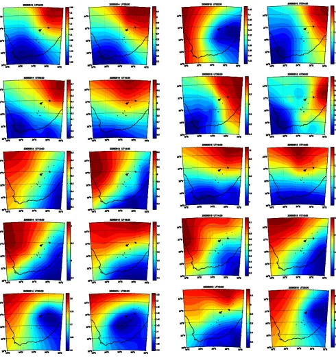
Fig. 4. Map of the electron density changes at an altitude of

350 km from 04:00 UT on 14 May to 20:00 UT on 15 May (unit: 1011el m−3).

indicate that the ionosphere has apparent positive anoma-lies. However, Fig. 5 shows that the peak altitude of iono-spheric electron density changed little. The slight change is attributed to the fact that the ground-based GNSS observation data and the small volume of radio occultation data used only minimally improved the vertical resolution of the inversion

Figure 4 Map of the electron density changes at an altitude of 350 km from 04:00UT on 14 May to 20:00UT on 15 May(unit:

1011_el/m3_).

Figure 5 shows the temporal and spatial variations in electron density on the 24°E profile

from 04:00UT on 14 May to 20:00UT on 15 May. Similar to Figure 4, Figure 5 shows that ionospheric electron density presented normal diurnal variations over time on 14May; it presented

violent abnormal changes on 15 May because of the magnetic storm. Electron density began to

increase at low latitudes first at 06:00UT on 14 May, then reached a maximum of 4.59×1011 _el/m3

at an altitude of 250 km between 22°S and 24°S. At 10:00UT, the electron density at any altitude was roughly consistent with that at longitude 24°E when peak electron density was

8.04×1011 el/m3at an altitude of 300 km. At 14:00UT, the ionospheric maximum electron density

remained unchanged, but slightly declined to 7.68×1011 _el/m3_{at high latitudes. At 18:00UT, the}

electron density significantly declined to 2.47×1011el/m3. The electron density further decreased

to 1.6×1011_el/m3 _{from 22:00UT on 14 May to 02:00UT on 15 May. The ionosphere began}

presenting significantly abnormal changes with the magnetic storm at 06:00UT on15 May. The

anomaly also increased with the continuous development of the magnetic storm. At 06:00UT, the

ionospheric maximum electron density was 5×1011 el/m3 at an altitude of 260 km without

significant anomalies compared with the same period on 14 May. At 10:00UT, however, electron density significantly increased to 1.3×1012 el/m3, which is 61.7% higher than that on 14 May. This

value is particularly significant between 22°S and 30°S. The results indicate that the ionosphere has apparent positive anomalies. However, Figure 5 shows that the peak altitude of ionospheric

electron density changed little. The slight change is attributed to the fact that the ground-based GNSS observation data and the small volume of radio occultation data used only minimally

improved the vertical resolution of the inversion results. The manner by which the vertical resolution of the inversion results is improved is a key issue for further study.

results. The manner by which the vertical resolution of the inversion results is improved is a key issue for further study. On the basis of the temporal and spatial distribution map of electron density at high altitudes and longitudes (Figs. 4 and 5), we can determine the strong ionospheric disturbances during the magnetic storm and the changes in the character-istics of ionospheric electron density at the middle and low latitudes of the Southern Hemisphere. Ionospheric activity

(7)

Y. B. Yao et al.: Temporal and spatial variations in ionospheric electron density profiles 381 Figure 4 Map of the electron density changes at an altitude of 350 km from 04:00UT on 14 May to 20:00UT on 15 May(unit:

1011_el/m3_).

Figure 5 shows the temporal and spatial variations in electron density on the 24°E profile

from 04:00UT on 14 May to 20:00UT on 15 May. Similar to Figure 4, Figure 5 shows that ionospheric electron density presented normal diurnal variations over time on 14May; it presented violent abnormal changes on 15 May because of the magnetic storm. Electron density began to increase at low latitudes first at 06:00UT on 14 May, then reached a maximum of 4.59×1011 _el/m3

at an altitude of 250 km between 22°S and 24°S. At 10:00UT, the electron density at any altitude was roughly consistent with that at longitude 24°E when peak electron density was

8.04×1011 el/m3at an altitude of 300 km. At 14:00UT, the ionospheric maximum electron density

remained unchanged, but slightly declined to 7.68×1011 el/m3at high latitudes. At 18:00UT, the electron density significantly declined to 2.47×1011el/m3. The electron density further decreased to 1.6×1011_el/m3_{from 22:00UT on 14 May to 02:00UT on 15 May. The ionosphere began}

presenting significantly abnormal changes with the magnetic storm at 06:00UT on15 May. The

anomaly also increased with the continuous development of the magnetic storm. At 06:00UT, the ionospheric maximum electron density was 5×1011 el/m3 at an altitude of 260 km without significant anomalies compared with the same period on 14 May. At 10:00UT, however, electron density significantly increased to 1.3×1012 _el/m3_{, which is 61.7% higher than that on 14 May. This}

value is particularly significant between 22°S and 30°S. The results indicate that the ionosphere has apparent positive anomalies. However, Figure 5 shows that the peak altitude of ionospheric

electron density changed little. The slight change is attributed to the fact that the ground-based GNSS observation data and the small volume of radio occultation data used only minimally improved the vertical resolution of the inversion results. The manner by which the vertical resolution of the inversion results is improved is a key issue for further study.

Fig. 5. Map of the electron density changes on the 24◦E pro-file from 04:00 UT on 14 May to 20:00 UT on 15 May (unit: 1011el m−3).

exhibited a strong relationship with latitude, and total elec-tron density decreased with increasing latitude. At a rela-tively calm space weather, the ionospheric electron density over the inversion region initially changed from low to high, then from high to low with time, indicating that the changes in ionospheric electron density are related to time. On the basis of the discussion of above, we inverted the ionospheric electron density in South Africa by CIT and regional high-precision GNSS observation data to determine the changes

Figure 5 Map of the electron density changes on the 24°E profile from 04:00UT on 14May to 20:00UT on15 May (unit: 1011_el/m3_).

On the basis of the temporal and spatial distribution map of electron density at high altitudes and longitudes (Figures 4 and 5), we can determine the strong ionospheric disturbances in during

the magnetic storm and the changes in the characteristics of ionospheric electron density at the middle and low latitudes of the Southern Hemisphere. Ionospheric activity exhibited a strong

relationship with latitude, and total electron density decreased with increasing latitude. At a relatively calm space weather, the ionospheric electron density over the inversion region initially

changed from low to high, then from high to low with time, indicating that the changes in ionospheric electron density are related to time. On the basis of the discussion of above, we

inversed the ionospheric electron density in South Africa by CIT and regional high-precision GNSS observation data to determine the changes in ionospheric activity, especially the

characteristics of the spatial and temporal distributions of the ionosphere during the magnetic storm.

5 Jason-1 satellite VTEC

The Jason-1 satellite is an ocean altimetry satellite jointly developed by the French Space

Agency (CNES) and the US Space Administration (NASA). The Jason-1 satellite covers up to 66°N to 66°S, with an orbit altitude of 1336 km. The satellite takes 112 minutes to run a cycle.

Theradar altimeter on the Jason-1 satellite has dual-band transmission frequency. The major frequency is ku-band and the minor frequency is C-band. The radar altimeter can directly

determine TEC in the vertical direction, and has high credibility for low-latitude and equatorial regions.

Using VTEC data obtained by the Jason-1 satellite from 13 to 18 May 2005, we analyzed the changes in ionospheric electron density during the magnetic storm and compared data on VTEC

ascending and descending orbits. Figures 6 and 7 show the tracks of the Jason-1 satellite in ascending and descending orbits and the spatial distribution of the data used. Because of the large

amount of data generated by the 1 Hz sampling rate of the Jason-1 satellite, we used the median in 18 seconds to smooth the data; the satellite can advance to about 1° during this period. From 13 to

18 May, the period at which the Jason-1 satellite’s ascending orbit went through the region near South Africa was 21:00UT to 04:00UT the next day at 3:00LT to 4:00LT; the period at which the satellite’s descending orbit went through South Africa was 10:00UT to 18:00UT at 15:00LT to

in ionospheric activity, especially the characteristics of the spatial and temporal distributions of the ionosphere during the magnetic storm.

3 Jason-1 satellite VTEC

The Jason-1 satellite is an ocean altimetry satellite jointly developed by the French Space Agency (CNES) and the US Space Administration (NASA). The Jason-1 satellite covers

(8)

382 Y. B. Yao et al.: Temporal and spatial variations in ionospheric electron density profiles and that data distribution is dense after smoothing.

Figure 6 Ascending orbit data image taken by the Jason-1 satellite from 13 to 18 May 2005.

Figure 7 Descending orbit data image taken by the Jason-1 satellite from 13 to 18 May 2005.

Figures 6 and 7 show the VTEC changes when the Jason-1 satellite is in ascending and descending orbits from 13 to 18 May 2005.Compared with the VTEC on 13May, when space was

at its calmest, the ascending orbit VTEC from 14 to 18 May showed no significant changes. On 15May, when the magnetic storm’s maximum main phase occurred, the Jason-1 satellite in the ascending orbit model appeared in the study region at 00:30UT, 02:30UT, 04:30UT, 21:00UT, and

23:00UT. The analysis of the Jason-1 satellite data is consistent with the CIT analysis. On 15May, the Jason-1 satellite in the descending orbit appeared in the study region at 11:00UT, 13:00UT, 15:00UT, 16:45UT, and 19:00UT. Compared with the VTEC obtained in the descending orbit

from 13 to 18 May, that on 15 May significantly increased at certain periods. The expanded area covers 10°S to 35°S, and the related VTEC data were obtained by the satellite at 11:00UT and 16:00UT. At 11:00UT, the satellite orbit was in the area from 0°S to 20°S and 74°E to 80°E. At

15:00UT, the satellite orbit was in the area from 10°S to 45°S and 74°E to 10°E. The results of the CIT inversion also revealed that significant positive anomalies occurred in the ionosphere at these periods. The VTEC data obtained by the satellite at 13:00UT and 15:00UT only minimally

changed. Figure 10 shows the VTEC observations and tracks of the Jason-1 satellite in the descending orbit model on 15 May. The analysis of VTEC data is consistent with the CIT analysis.

Fig. 6. Ascending orbit data image taken by the Jason-1 satellite

from 13 to 18 May 2005.

up to 66◦N to 66◦S, with an orbit altitude of 1336 km. The satellite takes 112 min to run a cycle. The radar altimeter on the Jason-1 satellite has dual-band transmission frequency. The major frequency is ku-band and the minor frequency is C-band. The radar altimeter can directly determine TEC in the vertical direction, and has high credibility for low-latitude and equatorial regions.

Using VTEC data obtained by the Jason-1 satellite from 13 to 18 May 2005, we analyzed the changes in ionospheric electron density during the magnetic storm and compared data on VTEC ascending and descending orbits. Figures 6 and 7 show the tracks of the Jason-1 satellite in ascending and descending orbits and the spatial distribution of the data used. Because of the large amount of data generated by the 1 Hz sampling rate of the Jason-1 satellite, we used the me-dian in 18 s to smooth the data; the satellite can advance to about 1◦during this period. From 13 to 18 May, the period at which the Jason-1 satellite’s ascending orbit went through the region near South Africa was 21:00 UT to 04:00 UT the next day at 03:00 LT to 04:00 LT; the period at which the satellite’s descending orbit went through South Africa was 10:00 UT to 18:00 UT at 15:00 LT to 16:00 LT. Figure 6 shows poor data on the satellite’s ascending orbit, and that data distribution is sparse after smoothing. By contrast, the figure shows fine data on the satellite’s descending orbit, and that data distri-bution is dense after smoothing.

Figures 6 and 7 show the VTEC changes when the Jason-1 satellite is in ascending and descending orbits from Jason-13 to 18 May 2005. Compared with the VTEC on 13 May, when space was at its calmest, the ascending orbit VTEC from 14 to 18 May showed no significant changes. On 15 May, when the magnetic storm’s maximum main phase occurred, the Jason-1 satellite in the ascending orbit model appeared in the study region at 00:30 UT, 02:30 UT, 04:30 UT, 21:00 UT, and 23:00 UT. The analysis of the Jason-1 satellite data is consistent with the CIT analysis. On 15 May, the Jason-1 satellite in the descending orbit appeared in the study region

and that data distribution is dense after smoothing.

Figure 6 Ascending orbit data image taken by the Jason-1 satellite from 13 to 18 May 2005.

Figure 7 Descending orbit data image taken by the Jason-1 satellite from 13 to 18 May 2005.

Figures 6 and 7 show the VTEC changes when the Jason-1 satellite is in ascending and descending orbits from 13 to 18 May 2005.Compared with the VTEC on 13May, when space was at its calmest, the ascending orbit VTEC from 14 to 18 May showed no significant changes. On 15May, when the magnetic storm’s maximum main phase occurred, the Jason-1 satellite in the ascending orbit model appeared in the study region at 00:30UT, 02:30UT, 04:30UT, 21:00UT, and 23:00UT. The analysis of the Jason-1 satellite data is consistent with the CIT analysis. On 15May, the Jason-1 satellite in the descending orbit appeared in the study region at 11:00UT, 13:00UT, 15:00UT, 16:45UT, and 19:00UT. Compared with the VTEC obtained in the descending orbit from 13 to 18 May, that on 15 May significantly increased at certain periods. The expanded area covers 10°S to 35°S, and the related VTEC data were obtained by the satellite at 11:00UT and 16:00UT. At 11:00UT, the satellite orbit was in the area from 0°S to 20°S and 74°E to 80°E. At 15:00UT, the satellite orbit was in the area from 10°S to 45°S and 74°E to 10°E. The results of the CIT inversion also revealed that significant positive anomalies occurred in the ionosphere at these periods. The VTEC data obtained by the satellite at 13:00UT and 15:00UT only minimally changed. Figure 10 shows the VTEC observations and tracks of the Jason-1 satellite in the descending orbit model on 15 May. The analysis of VTEC data is consistent with the CIT analysis.

Fig. 7. Descending orbit data image taken by the Jason-1 satellite

from 13 to 18 May 2005.

Figure 8 Changes in the VTEC data obtained by the Jason-1 satellite in the ascending orbit from May 13 to 18.

Figure 9 Changes in the VTEC data obtained by the Jason-1 satellite in the descending orbit from 13 to 18 May.

Figure 10 The descending orbit of the Jason-1 satellite and the VTEC observations on the study region on May 15.

6 Conclusion

We used the GNSS observations of the South African TrigNet to inverse the 3D temporal and

0 7 14

60°S 50°S 40°S 30°S 20°S 10°S G e o g ra p h ic L a ti tu d e ( d e g ) TEC May 13

0 7 14

TEC May 14

0 7 14

TEC May 15

0 7 14

TEC May 16

0 7 14

TEC May 17

0 7 14

TEC May 18

0 25 50

60°S 50°S 40°S 30°S 20°S 10°S TEC G e o g ra p h ic L a ti tu d e ( d e g ) May 13

0 25 50

May 14

TEC

0 25 50

May 15

TEC

0 25 50

May 16

TEC

0 25 50

May 17

TEC

0 25 50

May 18

TEC

Fig. 8. Changes in the VTEC data obtained by the Jason-1 satellite

in the ascending orbit from May 13 to 18.

at 11:00 UT, 13:00 UT, 15:00 UT, 16:45 UT, and 19:00 UT. Compared with the VTEC obtained in the descending orbit from 13 to 18 May, the one obtained on 15 May significantly increased at certain periods. The expanded area covers 10◦_S to 35◦_{S, and the related VTEC data were obtained by the} satellite at 11:00 UT and 16:00 UT. At 11:00 UT, the satel-lite orbit was in the area from 0◦S to 20◦S and 74◦E to 80◦E. At 15:00 UT, the satellite orbit was in the area from 10◦S to 45◦S and 74◦E to 10◦E. The results of the CIT in-version also revealed that significant positive anomalies oc-curred in the ionosphere at these periods. The VTEC data obtained by the satellite at 13:00 UT and 15:00 UT only min-imally changed. Figure 10 shows the VTEC observations and tracks of the Jason-1 satellite in the descending orbit model on 15 May. The analysis of VTEC data is consistent with the CIT analysis.

(9)

Figure 8 Changes in the VTEC data obtained by the Jason-1 satellite in the ascending orbit from May 13 to 18.

Figure 9 Changes in the VTEC data obtained by the Jason-1 satellite in the descending orbit from 13 to 18 May.

Figure 10 The descending orbit of the Jason-1 satellite and the VTEC observations on the study region on May 15.

6 Conclusion

0 7 14

TEC May 14

0 7 14

TEC May 15

0 7 14

TEC May 16

0 7 14

TEC May 17

0 7 14

TEC May 18

0 25 50

May 14

TEC

0 25 50

May 15

TEC

0 25 50

May 16

TEC

0 25 50

May 17

TEC

0 25 50

May 18

TEC

Fig. 9. Changes in the VTEC data obtained by the Jason-1 satellite

in the descending orbit from 13 to 18 May.

4 Conclusions

We used the GNSS observations of the South African TrigNet to inverse the 3-D temporal and spatial variations in ionospheric electron density in South Africa during the strong magnetic storm on 15 May 2005. We compared the electron density distributions at different altitudes and lon-gitudes on 14–15 May 2005. The electron density at any al-titude at 10:00 UT on 15 May significantly increased com-pared with that on 14 May, indicating that a positive-phase storm occurred in the ionosphere of the inversion region dur-ing the magnetic storm. The maximum electron density at each altitude at 10:00 UT on 15 May increased to 79.3 % on average compared with that on 14 May, at which the electron density at an altitude of 800 km increased to a maximum of 84.9 %. This increase is similar to the changes in electron density at any longitude.

To describe the process by which ionospheric electron density changed with time during the magnetic storm, we presented the electron density distribution at an altitude of 350 km and a longitude of 24◦E at a time interval of 2 h from 04:00 UT on 14 May to 20:00 UT on 15 May. The inversion results precisely reflect the 3-D fine structure of ionospheric electron density and its response to the development of the magnetic storm. We determined the strong ionospheric dis-turbances during the magnetic storm and identified the char-acteristics of the changes in ionospheric electron density at the middle and low latitudes of the Southern Hemisphere. The ionospheric activity was strongly related to latitude, and the total electron density decreased with increasing latitude.

We also used VTEC data from Jason-1 to analyze the iono-spheric changes before and after the magnetic storm. The VTEC from the descending orbit during the magnetic storm on 15 May significantly increased compared with that on 14 May, whereas the VTEC from the ascending orbit pre-sented insignificant changes. The time of occurrence and dis-tribution of the anomalies are consistent with of the CIT re-sults.

Figure 8 Changes in the VTEC data obtained by the Jason-1 satellite in the ascending orbit from May 13 to 18.

Figure 9 Changes in the VTEC data obtained by the Jason-1 satellite in the descending orbit from 13 to 18 May.

Figure 10 The descending orbit of the Jason-1 satellite and the VTEC observations on the study region on May 15.

6 Conclusion

0 7 14

TEC May 14

0 7 14

TEC May 15

0 7 14

TEC May 16

0 7 14

TEC May 17

0 7 14

TEC May 18

0 25 50

May 14

TEC

0 25 50

May 15

TEC

0 25 50

May 16

TEC

0 25 50

May 17

TEC

0 25 50

May 18

TEC

Fig. 10. The descending orbit of the Jason-1 satellite and the VTEC

observations on the study region on May 15.

Acknowledgements. The authors thank the IGS for providing GNSS observations, TripNet for providing observations on South Africa, IUGG for providing Kp and Dst indices, NASA for provid-ing IRI2007 model data, CNES for providprovid-ing Jason-1 observations, NOAA OSTM for providing Jason-2 observations, and NASA OMNIWEB for providing solar and geomagnetic indices. This work was supported by the Foundation for Innovative Research Groups of the National Natural Science Foundation of China (40721001) and the National Natural Science Foundation of China (41174012 and 41274022).

Edited by: A. Costa

Reviewed by: two anonymous referees

References

Appleton, E. and Ingram, L.: , Magnetic storms and upper atmo-spheric ionization, Nature, 136, 548–549, 1935.

Balan, D., Balaure, V., and Veghes, C.: Travel and tourism compet-itiveness of the world’s top tourismdestinations: An exploratory Assessment, Annales Universitatis Apulensis series Oeconom-ica, 11, 979–987, 2009.

Balan, N. and Rao, P. B.: Dependence of ionospheric response on the local time of sudden commencement and the intensity of ge-omagnetic storms, J. Atmos. Terrest. Phys., 52, 269–275, 1990. Balan, N., Shiokawa, K., Otsuka, Y., Kikuchi, T., Vijaya

Lek-shmi, D., Kawamura, S., Yamamoto, M., and Bailey, G. J.: A physical mechanism of positive ionospheric storms at low latitudes and midlatitudes, J. Geophys. Res., 115, A02304, doi:10.1029/2009JA014515, 2010.

(10)

Blewitt, G.: An automatic editing algorithm for GPS data, Jet Propulsion, 17, 199–202, 1990.

Burns, A. G., Killeen, T. L., Deng, W., Carignan, G. R., and Roble, R. G.: Geomagnetic Storm Effects in the Low- to Middle-Latitude Upper Thermosphere, J. Geophys. Res., 100, 14673– 14691, 1995.

Dumont, J. P., Rosmorduc, V., Picot, N., Desai, S., Bonekamp, H., Figa, J., Lillibridge, J., and Scharroo, R.: OSTM/Jason-2 prod-ucts handbook, 2009.

Essex, E. A., Mendillo, M., Sch¨odel, J. P., Klobuchar, J. A., da Rosa, A. V., Yeh, K. C., Fritz, R. B., Hibberd, F. H., Kersley, L., Koster, J. R., Matsoukas, D. A., Nakata, Y., and Roelofs, T. H.: A global response of the total electron content of the ionosphere to the magnetic storm of 17 and 18 June 1972, J. Atmos. Terr. Phys., 43, 293–306, 1981.

Fu, L. L., Christensen Jr., E., Lefebvre, C. Y., Meacutenard, M., Dorrer, Y. M., and Escudier, P.: TOPEX/POSEIDON mission overview, J. Geophys. Res., 99, 24369–24381, 1994.

Fuller-Rowell, T. J., Codrescu, M. V., Moffett, R. J., and Quegan, S.: Response of the Thermosphere and Ionosphere to Geomagnetic Storms, J. Geophys. Res., 99, 3893–3914, 1994.

Jee, G., Schunk, R. W., and Scherliess, L.: Analysis of TEC data from the TOPEX/Poseidon mission, J. Geophys. Res., 109, 1– 17, 2004.

Kelley, M. C., Vlasov, M. N., Foster, J. C., and Coster, A. J.: A quantitative explanation for the phenomenon known as stormenhanced density, Geophys. Res. Lett., 31, L19809, doi:10.1029/2004GL020875, 2004.

Lekshmi, V. D., Balan, N., Tulasi Ram, S., and Liu, J. Y.: Statis-tics of geomagnetic storms and ionospheric storms at low and mid latitudes in two solar cycles, J. Geophys. Res., 116, A11328, doi:10.1029/2011JA017042, 2011.

Lin, C. H., Richmond, A. D., Heelis, R. A., Bailey, G. J., Lu, G., Liu, J. Y., Yeh, H. C., and Su, S. Y.: Theoretical study of the low- and midlatitude ionospheric electron density enhance-ment during the October 2003 superstorm: Relative importance of the neutral wind and the electric field, J. Geophys. Res., 110, A12312, doi:10.1029/2005JA011304, 2005.

Lu, G., Goncharenko, L. P., Richmond, A. D., Roble, R. G., and Aponte, N.: A dayside ionospheric positive storm phase driven by neutral winds, J. Geophys. Res., 113, A08304, doi:10.1029/2007JA012895, 2008.

Lu, G., Goncharenko, L., Nicolls, M. J., Maute, A., Coster, A., and Paxton, L. J.: Ionospheric and thermospheric variations associ-ated with prompt penetration electric fields, J. Geophys. Res., 117, A08312, doi:10.1029/2012JA017769, 2012.

Mai, C. L. and Kiang, J. F.: Reconstruction of Ionospheric Pertur-bation Induced by 2004 Sumatra Tsunami Using a Computerized Tomography Technique, IEEE Trans. Geosci. Remote Sens., 47, 3303–3312, 2009.

Mannucci, A. J., Tsurutani, B. T., Iijima, B. A., Komjathy, A., Saito, A., Gonzalez, W. D., Guarnieri, F. L., Kozyra, J. U., and Skoug, R.: Dayside global ionospheric response to the major interplan-etary events of October 28–30, 2003 Halloween Storms 8221, Geophys. Res. Lett., 32, L12S02, doi:10.1029/2004GL021467, 2005.

Mendillo, M. and Narvaez, C.: Ionospheric storms at geophysically-equivalent sites – Part 1: Storm-time patterns for sub-auroral ionospheres, Ann. Geophys., 27, 1679–1694, doi:10.5194/angeo-27-1679-2009, 2009.

Mendillo, M. and Narvaez, C.: Ionospheric storms at geophysically-equivalent sites – Part 2: Local time storm patterns for sub-auroral ionospheres, Ann. Geophys., 28, 1449–1462, doi:10.5194/angeo-28-1449-2010, 2010.

Paul, M. P., Matsushita, S., and Richmond, A. D.: Ionospheric storm of 4–5 August 1972 in the Asia-Australia-Pacific sector, J. At-mos. Terr. Phys., 39, 43–50, 1977.

Richmond, A. D. and Matsushita, S.: Thermospheric Response to a Magnetic Substorm, J. Geophys. Res., 80, 2839–2850, 1975. Szuszczewicz, E. P., Lester, M., Wilkinson, P., Blanchard, P., Abdu,

M., Hanbaba, R., Igarashi, K., Pulinets, S., and Reddy, B. M.: A comparative study of global ionospheric responses to intense magnetic storm conditions, J. Geophys. Res., 103, 11665–11684, 1998.

Thampi, S. V., Lin, C., Liu, H., and Yamamoto, M.: First to-mographic observations of the Midlatitude Summer Nighttime Anomaly over Japan, J. Geophys. Res., 114, 1–10, 2009. Wen, D. B., Yuan, Y. B., On, J. K., Huo, X. L., and Zhang, K. F.:

Ionospheric temporal and spatial variations during the 18 August 2003 storm over China, Earth Planet. Space, 59, 313–317, 2007. Yao, Y. B., Chen, P., Wu, H., Zhang, S., and Peng, W. F.: Analysis of ionospheric anomalies before the 2011 M-w 9.0 Japan earth-quake, Chinese Sci. Bull., 57, 500–510, 2012a.

Yao, Y. B., Chen, P., Zhang, S., Chen, J. J., Yan, F., and Peng, W. F.: Analysis of pre-earthquake ionospheric anomalies before the globalM=7.0+ earthquakes in 2010, Nat. Hazards Earth Syst. Sci., 12, 575–585, doi:10.5194/nhess-12-575-2012, 2012b. Yeh, K., Ma, S., Lin, K., and Conkright, R.: Global ionospheric

effects of the October 1989 geomagnetic storm, J. Geophys. Res., 99, 6201–6218, 1994.

Yizengaw, E., Dyson, P. L., Essex, E. A., and Moldwin, M. B.: Iono-sphere dynamics over the Southern HemiIono-sphere during the 31 March 2001 severe magnetic storm using multi-instrument mea-surement data, Ann. Geophys., 23, 707–721, doi:10.5194/angeo-23-707-2005, 2005.

Zhao, B. Q.: Studies on the annual and semiannual anomalies and storm characteristics of mid- and low latitudes ionosphere, Ph.D. dissertation, Wuhan Institute of Physics and Mathematics & In-stitute of Geology and Geophysics, Chinese Academy of Sci-ences, 2006.