with Zero Floor on the Nominal Interest Rate
∗Anton Nakov Banco de Espa˜na
Recent treatments of the issue of a zero floor on nominal interest rates have been subject to some important method-ological limitations. These include the assumption of perfect foresight or the introduction of the zero lower bound as an initial condition or a constraint on the variance of the inter-est rate, rather than an occasionally binding non-negativity constraint. This paper addresses these issues, offering a global solution to a standard dynamic stochastic sticky-price model with an explicit occasionally binding non-negativity constraint on the nominal interest rate. It turns out that the dynam-ics and sometimes the unconditional means of the nominal rate, inflation, and the output gap are strongly affected by uncertainty in the presence of the zero lower bound. Commit-ment to the optimal rule reduces unconditional welfare losses to around one-tenth of those achievable under discretionary policy, while constant price-level targeting delivers losses that are only 60 percent larger than those under the optimal rule. Even though the unconditional performance of simple instru-ment rules is almost unaffected by the presence of the zero lower bound, conditional on a strong deflationary shock, simple instrument rules perform substantially worse than the optimal policy.
JEL Codes: E31, E32, E37, E47, E52.
∗I would like to thank Kosuke Aoki, Fabio Canova, Wouter den Haan, Jordi Gal´ı, Albert Marcet, Ramon Marimon, Bruce Preston, Morten Ravn, Michael Reiter, Thijs van Rens, John Taylor, and an anonymous referee for helpful com-ments and suggestions. I am grateful also for comcom-ments to seminar participants at Universitat Pompeu Fabra, ECB, Banco de Espa˜na, Central European Univer-sity, Warwick UniverUniver-sity, Mannheim UniverUniver-sity, New Economic School, Rutgers
1. Introduction
An economy is said to be in a “liquidity trap” when the mone-tary authority cannot achieve a lower nominal interest rate in order to stimulate output. Such a situation can arise when the nominal interest rate has reached its zero lower bound (ZLB), below which nobody would be willing to lend, if money can be stored at no cost for a nominally riskless zero rate of return.
The possibility of a liquidity trap was first suggested by Keynes (1936) with reference to the Great Depression of the 1930s. At that time he compared the effectiveness of monetary policy in such a situation to trying to “push on a string.” After WWII and espe-cially during the high-inflation period of the 1970s, interest in the topic receded, and the liquidity trap was relegated to a hypothetical textbook example. As Krugman (1998) noticed, of the few modern papers that dealt with it, most concluded that “the liquidity trap can’t happen, it didn’t happen, and it won’t happen again.”
With the benefit of hindsight, however, it did happen, and to no less than Japan. Figure 1 illustrates this, showing the evolution of output, inflation, and the short-term nominal interest rate fol-lowing the collapse of the Japanese real estate bubble of the late 1980s. The figure exhibits a persistent downward trend in all three variables and, in particular, the emergence of deflation since 1998 coupled with a zero nominal interest rate since 1999.
Motivated by the recent experience of Japan, the aim of the present paper is to contribute a quantitative analysis of the ZLB issue in a standard sticky-price model under alternative monetary policy regimes. On the one hand, the paper characterizes optimal monetary policy in the case of discretion and commitment.1 On the other hand, it studies the performance of several simple mone-tary policy rules, modified to comply with the zero floor, relative to the optimal commitment policy. The analysis is carried out within
University, HEC Montreal, EBRD, Koc University, and Universidad de Navarra. Financial support from the Spanish Ministry of Foreign Affairs (Becas MAE) and the ECB are gratefully acknowledged.
1The part of the paper on optimal policy is similar to independent work by
Adam and Billi (2006, 2007). The added value is to quantify and compare the performance of optimal commitment policy with that of a number of suboptimal rules in the same stochastic sticky-price setup.
Figure 1. Japan’s Fall into a Liquidity Trap
a stochastic general equilibrium model with monopolistic compe-tition and Calvo (1983) staggered price setting, under a standard calibration to the postwar U.S. economy.
The main findings are as follows: the optimal discretionary policy with zero floor involves a deflationary bias, which may be significant for certain parameter values and which implies that any quantitative analyses of discretionary biases of monetary policy that ignore the zero lower bound may be misleading. In addition, optimal discre-tionary policy implies much more aggressive cutting of the interest rate when the risk of deflation is high, compared with the corre-sponding policy without zero floor. Such a policy helps mitigate the depressing effect of private-sector expectations on current output and prices when the probability of falling into a liquidity trap is high.2
2An early version of this paper comparing the performance of optimal
dis-cretionary policy with three simple Taylor rules was circulated in 2004; optimal commitment policy and more simple rules were added in a version circulated in 2005. Optimal discretionary policy was studied independently by Adam and Billi (2004b), and optimal commitment policy by Adam and Billi (2004a).
In contrast, optimal commitment policy involves less preemptive lowering of the interest rate in anticipation of a liquidity trap, but it entails a promise for sustained monetary policy easing following an exit from a trap. This type of commitment enables the central bank to achieve higher expected (and actual) inflation and lower real rates in periods when the zero floor on nominal rates is binding.3
As a result, under the baseline calibration, the expected welfare loss under commitment is only around one-tenth of the loss under opti-mal discretionary policy. This implies that the cost of discretion may be much higher than normally considered when abstracting from the zero-lower-bound issue.
The average welfare losses under simple instrument rules are eight to twenty times larger than those under the optimal rule. How-ever, the bulk of these losses stem from the intrinsic suboptimality of simple instrument rules and not from the zero floor per se. This is related to the fact that under these rules the zero floor is hit very rarely—less than 1 percent of the time—compared with opti-mal commitment policy, which visits the liquidity trap one-third of the time. On the other hand, conditional on a large deflationary shock, the relative performance of simple instrument rules deterio-rates substantially vis-`a-vis the optimal commitment policy.
Issues of deflation and the liquidity trap have received consid-erable attention recently, especially after the experience of Japan.4
In an influential article, Krugman (1998) argued that the liquid-ity trap boils down to a credibilliquid-ity problem in which private agents expect any monetary expansion to be reverted once the economy has recovered. As a solution, he suggested that the central bank should commit to a policy of high future inflation over an extended horizon. More recently, Jung, Teranishi, and Watanabe (2005) have explored the effect of the zero lower bound in a standard sticky-price model with Calvo price setting under the assumption of perfect fore-sight. Consistent with Krugman (1998), they conclude that optimal
3
This basic intuition was suggested already by Krugman (1998), based on a simpler model.
4A partial list of relevant studies includes Krugman (1998), Wolman (1998),
McCallum (2000), Reifschneider and Williams (2000), Eggertsson and Woodford (2003), Klaeffling and Lopez-Perez (2003), Coenen, Orphanides, and Wieland (2004), Jung, Teranishi, and Watanabe (2005), Kato and Nishiyama (2005), and Adam and Billi (2006, 2007).
commitment policy entails a promise of a zero nominal interest for some time after the economy has recovered. Eggertsson and Wood-ford (2003) study optimal commitment policy with zero lower bound in a similar model in which the natural rate of interest is allowed to take two different values. In particular, it is assumed to become negative initially and then to jump to its “normal” positive level with a fixed probability in each period. These authors also conclude that the central bank should create inflationary expectations for the future. Importantly, they derive a moving price-level targeting rule that delivers the optimal commitment policy in this model.
One shortcoming of much of the modern literature on monetary policy rules is that it largely ignores the ZLB issue or at best uses rough approximations to address the problem. For instance, Rotem-berg and Woodford (1997) introduce nominal rate targeting as an additional central bank objective, which ensures that the resulting path of the nominal rate does not violate the zero lower bound too often. In a similar vein, Schmitt-Grohe and Uribe (2004) exclude from their analysis instrument rules that result in a nominal rate with an average that is less than twice its standard deviation. In both cases, therefore, one might argue that for sufficiently large shocks that happen with a probability as high as 5 percent, the derived monetary policy rules are inconsistent with the zero lower bound.
On the other hand, of the few papers that do introduce an explicit non-negativity constraint on nominal interest rates, most simplify the stochastics of the model—e.g., by assuming perfect foresight (Jung, Teranishi, and Watanabe 2005) or a two-state low/high econ-omy (Wolman 1998; Eggertsson and Woodford 2003). Even then, the zero lower bound is effectively imposed as an initial (“low”) condition and not as an occasionally binding constraint.5 While this
assump-tion may provide a reasonable first pass at a quantitative analysis, it may be misleading to the extent that it ignores the occasionally binding nature of the zero interest rate floor.
Other studies (e.g., Coenen, Orphanides, and Wieland 2004) lay out a stochastic model but knowingly apply inappropriate solution techniques that rely on the assumption of certainty equivalence. It
5Namely, the zero floor binds for the first several periods, but once the
is well known that this assumption is violated in the presence of a nonlinear constraint such as the zero floor, but nevertheless these researchers have imposed it for reasons of tractability (admittedly, they work with a larger model than the one studied here). Yet forcing certainty equivalence in this case amounts to assuming that agents ignore the risk of the economy falling into a liquidity trap when making their optimal decisions.
The present study contributes to the above literature by solving numerically a stochastic general equilibrium model with monopolis-tic competition and smonopolis-ticky prices with an explicit occasionally bind-ing zero lower bound, usbind-ing an appropriate global solution technique that does not rely on certainty equivalence. It extends the analysis of Jung, Teranishi, and Watanabe (2005) to the stochastic case with an AR(1) process for the natural rate of interest.
After a brief outline of the basic framework adopted in the analy-sis (section 2), the paper characterizes and contrasts the optimal discretionary and optimal commitment policies (sections 3 and 4). It then analyzes the performance of a range of simple instrument and targeting rules (sections 5 and 6) consistent with the zero floor.6 Sections 4–6 include a comparison of the conditional performance of all rules in a simulated liquidity trap, while section 7 presents their average performance, including a ranking according to uncon-ditional expected welfare. Section 8 studies the sensitivity of the findings to various parameters of the model, as well as the implica-tions of endogenous inflation persistence for the ZLB issue, and the last section concludes.
2. Baseline Model
While in principle the zero-lower-bound phenomenon can be studied in a model with flexible prices, it is with sticky prices that the liq-uidity trap becomes a real problem. The basic framework adopted in this study is a stochastic general equilibrium model with monop-olistic competition and staggered price setting `a la Calvo (1983) as
6These include truncated Taylor-type rules reacting to contemporaneous,
expected, or past inflation, output gap, or price level, and with or without “inter-est rate smoothing”; truncated first-difference rules; the “augmented Taylor rule” by Reifschneider and Williams (2000); and flexible price-level targeting.
in Gal´ı (2003) and Woodford (2003). In its simplest log-linearized version,7the model consists of three building blocks, describing the
behavior of households, firms, and the monetary authority.
The first block, known as the “IS curve,” summarizes the house-hold’s optimal consumption decision,
xt=Etxt+1−σ
it−Etπt+1−rtn
. (1)
It relates the “output gap” xt (i.e., the deviation of output from its flexible-price equilibrium) positively to the expected future out-put gap and negatively to the gap between the ex ante real interest rate,it−Etπt+1, and the “natural” (i.e., flexible-price equilibrium)
real rate, rtn (which is observed by all agents at time t).
Consump-tion smoothing accounts for the positive dependence of current out-put demand on expected future outout-put demand, while intertemporal substitution implies the negative effect of the ex ante real interest rate. The interest rate elasticity of output, σ, corresponds to the inverse of the coefficient of relative risk aversion in the consumers’ utility function.
The second building block of the model is a “Phillips curve”-type equation, which derives from the optimal price-setting deci-sion of monopolistically competitive firms under the assumption of staggered price setting `a la Calvo (1983),
πt=βEtπt+1+κxt, (2)
whereβ is the time discount factor andκ, the “slope” of the Phillips curve, is related inversely to the degree of price stickiness.8 Since firms are unable to adjust prices optimally every period, whenever
7
It is important to note that, like in the studies cited in the introduction, the objective here is a modest one, in that the only source of nonlinearity in the model stems from the ZLB. Solving the fully nonlinear sticky-price model with Calvo (1983) contracts can be a worthwile enterprise; however, it increases the dimensionality of the computational problem by the number of states and co-states that one should keep track of (e.g., the measure of price dispersion and, in the case of optimal policy, the Lagrange multipliers associated with all forward-looking constraints).
8In the underlying sticky-price model, the slopeκis given by [θ(1 +ϕε)]−1(1−
θ)(1−βθ)(σ−1+ϕ),whereθ is the fraction of firms that keep prices unchanged
in each period, ϕ is the (inverse) wage elasticity of labor supply, and ε is the elasticity of substitution among differentiated goods.
they have the opportunity to do so, they choose to price goods as a markup over a weighted average of current and expected future mar-ginal costs. Under appropriate assumptions on technology and pref-erences, marginal costs are proportional to the output gap, resulting in the above Phillips curve. Here this relation is assumed to hold exactly, ignoring the so-called cost-push shock, which sometimes is appended to generate a short-term trade-off between inflation and output-gap stabilization.
The final building block models the behavior of the monetary authority. The model assumes a “cashless-limit” economy in which the instrument controlled by the central bank is the nominal interest rate. One possibility is to assume a benevolent monetary policy-maker seeking to maximize the welfare of households. In that case, as shown in Woodford (2003), the problem can be cast in terms of a central bank that aims to minimize (under discretion or commit-ment) the expected discounted sum of losses from output gaps and inflation, subject to the optimal behavior of households (1) and firms (2), and the zero nominal interest rate floor:
Min it,πt,xt E0 ∞ t=0 βtπt2+λx 2 t (3) s.t. (1),(2) it≥0, (4)
whereλis the relative weight of the output gap in the central bank’s loss function.9
An alternative way of modeling monetary policy is to assume that the central bank follows some sort of simple decision rule that relates the policy instrument, implicitly or explicitly, to other variables in
9
Arguably, Woodford’s (2003) approximation to the utility of the representa-tive consumer is accurate to second order only in the vicinity of the steady state with zero inflation. To the extent that the shock inducing a zero interest rate pushes the economy far away from that steady state, the approximation error could in principle be large. In that case, the welfare evaluation in section 7 can be interpreted as a relative ranking of alternative policies based on an ad hoc loss criterion, under the assumption that the central bank targets zero inflation. Studying the welfare implication of different rules in the fully nonlinear model lies outside the scope of this paper.
the model. An example of such a rule, consistent with the zero floor, is a truncated Taylor rule,
it= max[0, r∗+π∗+φπ(πt−π∗) +φxxt], (5) where r∗ is an equilibrium real rate, π∗ is an inflation target, and
φπ and φx are response coefficients for inflation and the output gap. To close the model, one needs to specify the behavior of the natural real rate. In the fuller model, the latter is a composite of a variety of real shocks, including shocks to preferences, govern-ment spending, and technology. Following Woodford (2003), here I assume that the natural real rate follows an exogenous mean-reverting process, rtn=ρr n t−1+t, (6) where rn
t ≡ rtn−r∗ is the deviation of the natural real rate from
its mean, r∗; t are i.i.d. N(0, σ2) real shocks; and 0 ≤ ρ < 1 is a
persistence parameter.
The equilibrium conditions of the model therefore include the constraints (1), (2), and either a set of first-order optimality con-ditions (in the case of optimal policy) or a simple rule like (5). In either case the resulting system of equations cannot be solved with standard solution methods relying on local approximation because of the non-negativity constraint on the nominal rate. Hence I solve them with a global solution technique known as “collocation.” The rational-expectations equilibrium with occasionally binding con-straint is solved by way of parameterizing expectations (Christiano and Fischer 2000) and is implemented with the MATLAB routines developed by Miranda and Fackler (2002). The appendix outlines the simulation algorithm, while the following sections report the results.
2.1 Baseline Calibration
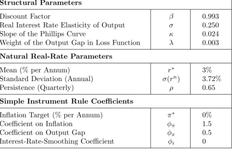
The model’s parameters are chosen to be consistent with the “stan-dard” Woodford (2003) calibration to the U.S. economy, which in turn is based on Rotemberg and Woodford (1997) (table 1). Thus, the slope of the Phillips curve (0.024), the weight of the output gap in the central bank loss function (0.003), the time discount factor (0.993), and the mean (3 percent per annum) and standard devia-tion (3.72 percent) of the natural real rate are all taken directly from
Table 1. Baseline Calibration (Quarterly Unless Otherwise Stated)
Structural Parameters
Discount Factor β 0.993
Real Interest Rate Elasticity of Output σ 0.250 Slope of the Phillips Curve κ 0.024 Weight of the Output Gap in Loss Function λ 0.003
Natural Real-Rate Parameters
Mean (% per Annum) r∗ 3%
Standard Deviation (Annual) σ(rn) 3.72%
Persistence (Quarterly) ρ 0.65
Simple Instrument Rule Coefficients
Inflation Target (% per Annum) π∗ 0%
Coefficient on Inflation φπ 1.5
Coefficient on Output Gap φx 0.5
Interest-Rate-Smoothing Coefficient φi 0
Woodford (2003). The persistence (0.65) of the natural real rate is assumed to be between the one used by Woodford (2003) (0.35) and that estimated by Adam and Billi (2006) (0.8) using a more recent sample period.10 The real interest rate elasticity of aggregate
demand (0.25)11 is lower than the elasticity assumed by Eggertsson and Woodford (2003) (0.5), but as these authors point out, if any-thing, a lower degree of interest sensitivity of aggregate expenditure biases the results toward a more modest output contraction as a result of a binding zero floor.12 In the simulations with simple rules,
the baseline target inflation rate (0 percent) is consistent with the implicit zero target for inflation in the central bank’s loss function.
10These parameters for the shock process imply that the natural real interest
rate is negative about 15 percent of the time on an annual basis. This is slightly more often than with the standard Woodford (2003) calibration (10 percent).
11
This corresponds to a constant relative risk aversion of 4 in the underlying model.
12With the Woodford (2003) value of this parameter (6.25), the model predicts
unrealistically large output shortfalls when the zero floor binds—e.g., an output gap around –30 percent for values of the natural real rate around –3 percent.
The baseline reaction coefficients on inflation (1.5), the output gap (0.5), and the lagged nominal interest rate (0) are standard in the lit-erature on Taylor (1993)-type rules. Section 8 studies the sensitivity of the results to various parameter changes.
3. Discretionary vs. Commitment Policy
Since the seminal work of Kydland and Prescott (1977) and Barro and Gordon (1983), the literature has focused on two (arguably extreme) ways of dealing with problems in which agents’ expec-tations of future policy actions affect their current behavior. One is assuming full discretion, meaning that policymakers are unable to make any promises about their own (or their successors’) future actions. The alternative is to suppose that policymakers have free access to a perfect commitment technology, which guarantees that they will never default on any of their past promises. While these two polar settings provide important insights into a wide vari-ety of macroeconomic problems, their predictions sometimes differ considerably.
This turns out to be so in the context of the zero-lower-bound issue. In particular, this section shows that if the central bank cannot make any credible promises about the future course of monetary pol-icy, then the zero lower bound is invariably associated with deflation. On the other hand, if the central bank is able to commit to the opti-mal state-contingent policy, then hitting the zero lower bound need not be associated with a falling price level, and may even result in slightly positive inflation. Intuitively, by committing tofuture infla-tion (once the zero lower bound ceases to bind), the central bank is able to reduce the real interest rate and stimulate demand at times when output is unusually low and the interest rate is constrained by the zero floor. At the same time, forward-looking price-setting behavior implies that some of the expected future inflation is built into current pricing decisions, which may result in slightly positive inflation even while the zero floor is binding. This way of affecting behavior is just unavailable to a discretionary policymaker; there-fore, in the discretion case the private sector correctly anticipates that the zero lower bound will prevent the central bank from offset-ting fully the effects of large-enough negative shocks on inflation.
3.1 Optimal Discretionary Policy
Abstracting from the zero floor, the solution to the discretionary optimization problem is well known (Clarida, Gal´ı, and Gertler 1999).13 Under discretion, the central bank cannot manipulate the beliefs of the private sector, and it takes expectations as given. The private sector is aware that the central bank is free to reoptimize its plan in each period; therefore, in a rational-expectations equilibrium, the central bank should have no incentives to change its plans in an unexpected way. In the baseline model with no endogenous state variables, the discretionary policy problem reduces to a sequence of static optimization problems in which the central bank minimizes current-period losses by choosing the current inflation, output gap, and nominal interest rate as a function only of the exogenous natural real rate, rnt.
The solution without zero bound then is straightforward: infla-tion and the output gap are fully stabilized at their (zero) targets in every period and state of the world, while the nominal interest rate moves one-for-one with the natural real rate. This is depicted by the dashed lines in figure 2. With this policy, the central bank is able to achieve the globally minimal welfare loss of zero at all times.
With the zero floor, the basic problem of discretionary opti-mization (without endogenous state variables) can still be cast as a sequence of static problems. The period-tLagrangian is given by
1 2 π2t +λx2t +φ1t[xt−f1t+σ(it−f2t)] +φ2t[πt−κxt−βf2t] +φ3tit, (7)
whereφ1tis the Lagrange multiplier associated with the IS curve (1), φ2t with the Phillips curve (2), andφ3t with the zero constraint (4).
The functions f1t = Et(xt+1) and f2t = Et(πt+1) are the
private-sector expectations that the central bank takes as given. Noticing thatφ3t=−σφ1t, the Kuhn-Tucker conditions for this problem can
be written as
πt+φ2t= 0 (8)
λxt+φ1t−κφ2t= 0 (9)
itφ1t = 0 (10)
it ≥0 (11)
φ1t ≥0. (12)
Substituting (8) and (9) into (10), and combining the result with (1), (2), and (4), a Markov-perfect rational-expectations equilibrium should satisfy xt−Etxt+1+σ it−Etπt+1−rtn = 0 (13) πt−κxt−βEtπt+1= 0 (14) it(λxt+κπt) = 0 (15) it≥0 (16) λxt+κπt≤0. (17)
Figure 2. Optimal Discretionary Policy with Perfect Foresight
Notice that (15) implies that the typical “targeting rule” involv-ing inflation and the output gap is satisfied whenever the zero floor on the nominal interest rate is not binding,
λxt+κπt= 0, (18)
ifit>0. (19)
However, when the zero floor is binding, from (13) the dynamics are governed by
xt+σpt−σrnt =Etxt+1+σEtpt+1 (20)
ifit = 0, (21)
where pt is the (log) price level. Notice that it is no longer pos-sible to set inflation and the output gap to zero at all times, for such a policy would require a negative nominal rate when the nat-ural real rate falls below zero. Moreover, (20) implies that if the natural real rate falls so that the zero floor becomes binding, then since next period’s output gap and price level are independent of today’s actions, for expectations to be rational, the sum of the cur-rent output gap and price level must fall. The latter is true for any process for the natural real rate that allows it to take negative values.
An interesting special case, which replicates the findings of Jung, Teranishi, and Watanabe (2005), is the case of perfect foresight. By perfect foresight it is meant here that the natural real rate jumps initially to some (possibly negative) value, after which it follows a deterministic path (consistent with an AR(1) process) back to its steady state. In this case, the policy functions are represented by the solid lines in figure 2. As anticipated in the previous para-graph, at negative values of the natural real rate, both the output gap and inflation are below target. On the other hand, at posi-tive levels of the natural real rate, prices and output can be sta-bilized fully in the case of discretionary optimization with perfect foresight. The reason for this is simple: once the natural real rate is above zero, deterministic reversion to steady state ensures that it will never be negative in the future. This means that it can always be tracked one-for-one by the nominal rate (as in the case
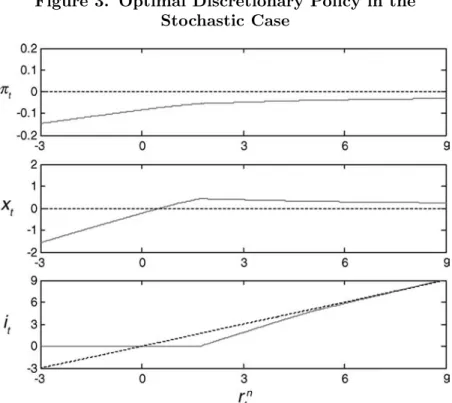
Figure 3. Optimal Discretionary Policy in the Stochastic Case
without zero floor), which is sufficient to fully stabilize prices and output.
One of the contributions of this paper is to extend the analysis in Jung, Teranishi, and Watanabe (2005) to the more general case in which the natural real rate follows a stochastic AR(1) process. Figure 3 plots the optimal discretionary policy in the stochastic environment. Clearly, optimal discretionary policy differs in several important ways, both from the optimal discretionary policy uncon-strained by the zero floor and from the conuncon-strained perfect-foresight solution.
First of all, given the zero floor, it is in general no longer optimal to set either inflation or the output gap to zero in any period. In fact, in the solution with zero floor, inflation falls short of the target atany
level of the natural real rate. This gives rise to a “deflationary bias” of optimal discretionary policy—in other words, anaverage rate of inflation below the target. Sensitivity analysis shows that for some
plausible parameter values, the deflationary bias becomes quanti-tatively significant.14 This implies that any quantitative analysis
of discretionary biases in monetary models that does not take into account the zero lower bound can be misleading.
Secondly, as in the case of perfect foresight, at negative levels of the natural real rate, both inflation and the output gap fall short of their respective targets. However, the deviations from target are larger in the stochastic case—up to 1.5 percentage points for the output gap and up to 15 basis points for inflation at a natural real rate of –3 percent. As we will see in the following section, the fall of inflation under discretionary optimization is in contrast with the case of commitment, when prices are much better stabilized and may even slightly increase while the nominal interest rate is at its zero lower bound.
Third, above a positive threshold for the natural real rate, the optimal output gap becomes positive, peaking at around +0.5 percent.
Finally, at positive levels of the natural real rate, the optimal nominal interest rate policy with zero floor is both more expan-sionary (i.e., prescribing a lower nominal rate) andmore aggressive
(i.e., steeper) compared with the optimal discretionary policy with-out zero floor.15 As a result, the nominal rate hits the zero floor at levels of the natural real rate as high as 1.8 percent (and is constant at zero for lower levels of the natural real rate).
These results hinge on two factors: (i) the nonlinearity induced by the zero floor and (ii) the stochastic nature of the natural real rate. The combined effect is an asymmetry in the ability of the cen-tral bank to respond to positive versus negative shocks when the natural real rate is close to zero. Namely, while the central bank can fully offset any positive shocks to the natural real rate because nothing prevents it from raising the nominal rate by as much as is necessary, it cannot fully offset large-enough negative shocks. The most it can do in this case is to reduce the nominal rate to zero, which is still higher than the rate consistent with zero output gap
14
For example, the deflationary bias becomes half a percentage point with ρ= 0.8 andr∗= 2 percent.
15This is also true when the optimal nominal interest rate policy is compared
and inflation. Taking private-sector expectations as given, the lat-ter implies a higher than desiredreal interest rate, which depresses output and prices through the IS and Phillips curves.
At the same time, when the natural real rate is close to zero, private-sector expectations reflect the asymmetry in the central bank’s problem: a positive shock in the following period is expected to be neutralized, while an equally probable negative one is expected to take the economy into a liquidity trap. This gives rise to a “defla-tionary bias” in expectations, which in a forward-looking economy has an immediate impact on the current evolution of output and prices. Absent an endogenous state, the current evolution of the economy is all that matters today, and so it is rational for the cen-tral bank to partially offset the depressing effect of expectations on today’s outcome by more aggressively lowering the nominal rate when the risk of deflation is high.
At sufficiently high levels of the natural real rate, the proba-bility for the zero floor to become binding converges to zero. In that case, optimal discretionary policy approaches the unconstrained one—namely, zero output gap and inflation and a nominal rate equal to the natural real rate. However, around the deterministic steady state, the differences between the two policies—with and without zero floor—remain significant.
Since in the baseline model the discretionary optimization prob-lem is equivalent to a sequence of static probprob-lems, optimal discre-tionary policy is independent of history. This means that it is only the current risk of falling into a liquidity trap that matters for cur-rent policy, regardless of whether the economy is approaching a liq-uidity trap or has just exited one. This is in sharp contrast with the optimal policy under commitment, which involves a particular type of history dependence, as will become clear in the following section.
3.2 Optimal Commitment Policy
In the absence of the zero lower bound, the equilibrium outcome under optimal discretion is globally optimal, and therefore it is observationally equivalent to the outcome under optimal commit-ment policy. The central bank manages to stabilize fully inflation and the output gap while adjusting the nominal rate one-for-one with the natural real rate.
However, this observational equivalence no longer holds in the presence of a zero interest rate floor. While full stabilization under either regime is not possible, important gains can be obtained from the ability to commit to future policy. In particular, by committing to deliver inflation in the future, the central bank can affect private-sector expectations about inflation, and thus the real rate, even when the nominal interest rate is constrained by the zero floor. This channel of monetary policy is simply unavailable to a discretionary policymaker.
Using the same Lagrange method as before, but this time taking into account the dependence of expectations on policy choices, it is straightforward to obtain the equilibrium conditions that govern the optimal commitment solution:
xt−Etxt+1+σ it−Etπt+1−rnt = 0 (22) πt−κxt−βEtπt+1= 0 (23) πt−φ1t−1σ/β+φ2t−φ2t−1= 0 (24) λxt+φ1t−φ1t−1/β−κφ2t= 0 (25) itφ1t= 0 (26) it≥0 (27) φ1t≥0. (28)
From conditions (24) and (25), it is clear that the Lagrange mul-tipliers inherited from the past period will have an effect on current policy. They in turn will depend on the history of endogenous vari-ables and in particular on whether the zero floor was binding in the past. In this sense, the Lagrange multipliers summarize the effect of commitment, which (in contrast to optimal discretionary policy), involves a particular type of history dependence.
Figures 4–6 plot the optimal policies in the case of commitment. The figures illustrate specifically the dependence of policy onφ1t−1,
the Lagrange multiplier associated with the zero floor, while hold-ing φ2t−1 fixed. When the nominal interest rate is constrained by
the zero floor, φ1 becomes positive, implying that the central bank
commits to a lower nominal rate, higher inflation, and higher output gap in the following period, conditional on the value of the natural real rate.
Figure 4. Optimal Commitment Policy (Inflation)
Figure 6. Optimal Commitment Policy (Nominal Interest Rate)
Since the commitment is assumed to be credible, it enables the central bank to achieve higher expected inflation and a lower real rate in periods when the nominal rate is constrained by the zero floor. The lower real rate reinforces expectations for higher future output and thus further stimulates current output demand through the IS curve. This, together with higher expected inflation, stimulates cur-rent prices through the expectational Phillips curve. Commitment therefore provides an additional channel of monetary policy, which works through expectations and through the ex ante real rate, and which is unavailable to a discretionary monetary policymaker.
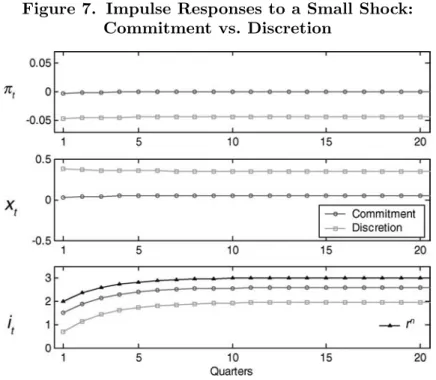
A standard way to illustrate the differences between optimal dis-cretionary and commitment policies is to compare the dynamic evo-lution of endogenous variables under each regime in response to a single shock to the exogenous natural real rate. Figures 7 and 8 plot the impulse responses to a small and a large negative shock to the natural real rate, respectively. In figure 7, notice that in the case
Figure 7. Impulse Responses to a Small Shock: Commitment vs. Discretion
Figure 8. Impulse Responses to a Large Shock: Commitment vs. Discretion
of a small shock to the natural real rate from its steady state of 3 percent down to 2 percent, inflation and the output gap under optimal commitment policy (lines with circles) remain almost fully stabilized. In contrast, under discretionary optimization (lines with squares), inflation stays slightly below target and the output gap remains about half a percentage point above target, consistent with equation (18), as the economy converges back to its steady state. The nominal interest rate under discretion is about 1 percent lower than the rate under commitment throughout the simulation, yet it remains strictly positive at all times.
The picture changes substantially in the case of a large nega-tive shock to the natural interest rate to –3 percent (see figure 8). Notably, under both commitment and discretion, the nominal inter-est rate hits the zero lower bound and remains there until two quar-ters after the natural interest rate has returned to positive.16 Under discretionary optimization, both inflation and the output gap fall on impact, consistent with equation (20), after which they converge toward their steady state. The initial shortfall is significant, espe-cially for the output gap, amounting to about 1.5 percent. In con-trast, under the optimal commitment rule, the initial output loss and deflation are much milder, owing to the ability of the central bank to commit to a positive output gap and inflation once the natural real rate has returned to positive.
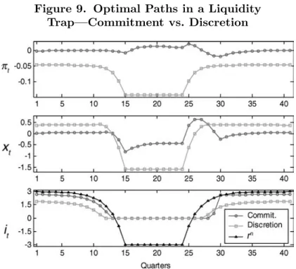
An alternative way to compare optimal discretionary and com-mitment policies in the stochastic environment is to juxtapose the dynamic paths that they prescribe for endogenous variables under a chosen evolution for the stochastic natural real rate.17 The
experiment is shown in figure 9, which plots a simulated “liquid-ity trap” under the two regimes. The line with triangles in the bottom panel is the assumed evolution of the natural real rate. It slips down from +3 percent (its deterministic steady state) to −3 percent over a period of fifteen quarters, then remains at −3
16
The fact that the zero-interest-rate policy terminates in the same quarter under commitment and under discretion is a coincidence in this experiment. The relative duration of a zero-interest-rate policy under commitment versus discre-tion depends on the parameters of the shock process as well as the particular realization of the shock.
17In the model, agents observe only the current state; i.e., the future evolution
Figure 9. Optimal Paths in a Liquidity Trap—Commitment vs. Discretion
percent for ten quarters before recovering gradually (consistent with the assumed AR(1) process) to +3 percent in another fifteen quarters.
The top and middle panels of figure 9 show the responses of inflation and the output gap under each of the two regimes. Not surprisingly, under the optimal commitment regime, both infla-tion and the output gap are closer to target than under the opti-mal discretionary policy. In particular, under optiopti-mal discretion, inflation is always below the target as it falls to −0.15 percent, shadowing the drop in the natural real rate. Compared to that, under optimal commitment, prices are almost fully stabilized, and in fact they even slightly increase while the natural real rate is negative!
In turn, under optimal discretion the output gap is initially around +0.4 percent, but then it declines sharply to −1.6 percent with the decline in the natural real rate. In contrast, under optimal commitment, output is initially at its potential level and the largest
negative output gap is only half the size of the one under optimal discretion.
Supporting these paths of inflation and the output gap are corresponding paths for the nominal interest rate. Under discre-tionary optimization, the nominal rate starts at around 2 percent and declines at an increasing rate until it hits zero two quarters before the natural real rate has turned negative. It is then kept at zero while the natural real rate is negative, and only two quarters after the latter has returned to positive territory does the nomi-nal interest rate start rising again. Nominomi-nal rate increases following the liquidity trap mirror the decreases while approaching the trap, so that the tightening is more aggressive in the beginning and then gradually diminishes as the nominal rate approaches its steady state. In contrast, the nominal rate under optimal commitment begins closer to 3 percent, then declines to zero one quarter before the natural real rate turns negative. After that, it is kept at its zero floor until three quarters after the recovery of the natural real rate to positive levels, which is one quarter longer compared with opti-mal discretionary policy. Interestingly, once the central bank starts increasing the nominal rate, it raises it very quickly; the nominal rate climbs nearly 3 percentage points in just two quarters. This is equivalent to six consecutive monthly increases by 50 basis points each. The reason is that once the central bank has validated the inflationary expectations (which help mitigate deflation during the liquidity trap), there is no more incentive to keep inflation above target when the natural interest rate has returned to normal.
Under discretion, the paths of inflation, output, and the nomi-nal rate are symmetric with respect to the midpoint of the simula-tion period because optimal discresimula-tionary policy is independent of history. Therefore, inflation and the output gap inherit the dynamics of the natural real rate, the only state variable on which they depend. This is in contrast with the asymmetric paths of the endogenous variables under commitment, reflecting the optimal history depen-dence of policy under this regime. In particular, the fact that under commitment the central bank can promise higher output gap and inflation in the wake of a liquidity trap is precisely what allows it to engage in less preemptive easing of policy in anticipation of the trap and at the same time deliver a superior inflation and output-gap performance compared with the optimal policy under discretion.
4. Suboptimal Rules with Zero Floor 4.1 Targeting Rules
In the absence of the zero floor, targeting rules take the form
απEtπt+j+αxEtxt+k+αiEtit+l =τ, (29)
where απ, αx, and αi are weights assigned to the different objec-tives;j, k,and lare forecasting horizons; and τ is the target. These are sometimes calledflexible inflation-targeting rules to distinguish them fromstrict inflation targeting of the formEtπt+j =τ.18When j, k, or l > 0, the rules are called inflation forecast targeting to distinguish them from rules targeting contemporaneous variables.
As demonstrated by (20) in section 3, in general, such rules are not consistent with equilibrium in the presence of the zero floor, for they would require negative nominal interest rates at times. A nat-ural way to modify targeting rules so that they comply with the zero floor is to write them as a complementarity condition,
it(απEtπt+j+αxEtxt+k+αiEtit+l−τ) = 0 (30)
it≥0, (31)
which requires that either the target τ is met or the nominal inter-est rate must be at its zero floor. In this sense, a rule like (30)–(31) can be labeled “flexible inflation targeting with a zero-interest-rate floor.”
In fact, section 3 showed that the optimal policy under discre-tion takes this form withαi = 0, απ = κ, αx =λ,j =k = 0, and
τ = 0—namely,
it(λxt+κπt) = 0 (32)
it ≥0. (33)
In the absence of the zero floor, it is well known that opti-mal commitment policy can be formulated as optiopti-mal speed-limit
18Notice that the zero lower bound implies that strict inflation targeting is
simply not feasible: from the New Keynesian Phillips curve, πt = C implies
xt=C(1−β) at all times, and the IS equation is not satisfied for large-enough
negative shocks torn t.
targeting,
∆xt+κ
λπt= 0, (34)
where ∆xt= ∆yt−∆ytf lexis the growth rate of output relative to the
growth rate of flexible-price output (the speed limit). In contrast to discretionary optimization, however, the optimal commitment rule with zero floor cannot be written in the form (30)–(31). This is because, with zero floor, the optimal target involves a particular type of history dependence, as shown by Eggertsson and Woodford (2003).19 In particular, manipulating the first-order conditions of
the optimal commitment problem, one can arrive at the following speed-limit targeting rule with zero floor:
it ∆xt+κ λπt− 1 λ κσ+β β φ1t−1−φ1t+ 1 β∆φ1t−1 = 0 (35) it ≥0. (36) Since κσ is small and β is close to one, and for plausible values ofφ1t consistent with the assumed stochastic process for the natural
real rate,20 the above rule is approximately the same as
it ∆yt+κ
λπt−τt
= 0 (37)
it ≥0, (38)
whereτt≈∆ytf lex+λ−1∆2φ1t is a history-dependent target (speed
limit). In normal circumstances when φ1t =φ1t−1=φ1t−2= 0, the
target is equal to the growth rate of flexible-price output, as in the problem without zero bound; however, if the economy falls into a liq-uidity trap, the speed limit is adjusted in each period by the speed of change of the penalty (the Lagrange multiplier) associated with the non-negativity constraint. The faster the economy is plunging into the trap, therefore, the higher is the speed-limit target that the
19
These authors derive the optimal commitment policy in the form of a mov-ing price-level targeting rule. Alternatively, it can be formulated as a moving speed-limit targeting rule as demonstrated here.
20φ
central bank promises to achieve contingent on the interest rate’s return to positive territory.
While the above rule is optimal in this framework, it is perhaps not very practical. Its dependence on the unobservable Lagrange multipliers makes it very hard, if not impossible, to implement or communicate to the public. Moreover, as pointed out by Eggertsson and Woodford (2003), credibility might suffer if all that the pri-vate sector observes is a central bank that persistently undershoots its target yet keeps raising it for the following period. To overcome some of these drawbacks, Eggertsson and Woodford (2003) propose a simpler constant price-level targeting rule, of the form
it xt+κ
λpt
= 0
it≥0, (39)
wherept is the log price level.21
The idea is that committing to a price-level target implies that any undershooting of the target resulting from the zero floor is going to be undone in the future by positive inflation. This raises private-sector expectations and eases deflationary pressures when the econ-omy is in a liquidity trap. Figure 10 demonstrates the performance of this simpler rule in a simulated liquidity trap. Notice that while the evolution of the nominal rate and the output gap is similar to that under the optimal discretionary rule, the path of inflation is much closer to the target. Since the weight of inflation in the cen-tral bank’s loss function is much larger than that of the output gap, the fact that inflation is better stabilized accounts for the superior performance of this rule in terms of welfare.
4.2 Simple Instrument Rules
The practical difficulties with communicating and implementing rules like (35) or even (39) have led many researchers to focus on simple instrument rules of the type proposed by Taylor (1993). These rules have the advantage of postulating a relatively straightforward
21Notice that the weight on the price level is optimal within the class of
con-stant price-level targeting rules. In particular, it is related toκ/λ=ε, the degree of monopolistic competition among intermediate goods producers.
Figure 10. Dynamic Paths under Constant Price-Level Targeting
relationship between the nominal interest rate and a limited set of variables in the economy. While the advantage of these rules lies in their simplicity, at the same time—absent the zero floor—some of them have been shown to perform close enough to the optimal rules in terms of the underlying policy objectives (Gal´ı 2003). Hence, it has been argued that some of the better simple instrument rules may serve as a useful benchmark for policy, while facilitating communi-cation and transparency.
In most of the existing literature, however, simple instrument rules are specified as linear functions of the endogenous variables. This is, in general, inconsistent with the existence of a zero floor because for large-enough negative shocks (e.g., to prices), linear rules would imply a negative value for the nominal interest rate. For instance, a simple instrument rule reacting only to past period’s inflation,
wherer∗ is the equilibrium real rate,π∗ is the target inflation rate, andφπis an inflation response coefficient, can clearly imply negative values for the nominal rate.
In the context of liquidity trap analysis, a natural way to modify simple instrument rules is to truncate them at zero with the max(·) operator. For example, the truncated counterpart of the above Tay-lor rule can be written as
it= max[0, r∗+π∗+φπ(πt−1−π∗)]. (41)
In what follows, I consider several types of truncated instrument rules, including the following:
• Truncated Taylor rules (TTRs) that react to past, contem-poraneous, or expected future values of the output gap and inflation (j∈ {−1,0,1}),
iT T Rt = max[0, r∗+π∗+φπ(Etπt+j−π∗) +φx(Etxt+j)] (42) • TTRs with partial adjustment or “interest rate smoothing”
(TTRSs), iT T RSt = max 0, φiit−1+ (1−φi)iT T Rt (43) • TTRs that react to the price level instead of inflation
(TTRPs),
iT T RPt = max[0, r∗+φπ(pt−p∗) +φxxt] (44)
wherept is the log price level and p∗ is a constant price-level target; and
• Truncated “first-difference” rules (TFDRs) that specify the
change in the interest rate as a function of the output gap and inflation,
iT F DRt = max[0, it−1+φπ(πt−π∗) +φxxt]. (45)
This formulation ensures that if the nominal interest rate ever hits zero, it will be held there as long as inflation and the output gap are negative, thus extending the duration of a zero-interest-rate policy relative to a truncated Taylor rule.
• The “augmented Taylor rule” (ATR) of Reifschneider and Williams (2000), iAT Rt = max 0, iT Rt −αZt (46) iT Rt =r∗+π∗+φπ(πt−π∗) +φxxt (47) Zt =Zt−1+ iAT Rt −iT Rt . (48)
This last rule keeps track of the amount by which the interest rate was higher than an unconstrained Taylor rule due to a bind-ing zero lower bound, and allows for a compensatbind-ing lower nominal interest rate once the natural real rate has returned to positive lev-els. Reifschneider and Williams (2000) simulate a stochastic econ-omy with this policy (under the assumption of certainty equivalence) and show that it improves performance substantially compared with the standard Taylor rule. The augmented Taylor rule is interesting also because it is thought to have influenced the conduct of mone-tary policy in the United States during the 2003–05 episode when announcements by Federal Reserve Chairman Alan Greenspan sug-gested a “considerable period” of low interest rates, followed by a “measured pace” of interest rate increases.22
As before, I illustrate the performance of each family of sim-ple instrument rules by simulating a liquidity trap and plotting the implied paths of endogenous variables under each regime. In addi-tion, I contrast the performance of optimal commitment policy to the augmented rule of Reifschneider and Williams (2000), assuming that the Federal Reserve followed their rule in the period since 2001:Q3. The more rigorous evaluation of welfare of alternative policies is reserved for the following section.
Given the model’s simplicity, the focus here is not on finding the optimal values of the parameters within each class of rules but rather on evaluating the performance of alternative monetary policy regimes. To do that I use values of the parameters commonly esti-mated and widely used in simulations in the literature. I make sure that the parameters satisfy a sufficient condition for local uniqueness of equilibrium. Namely, the parameters are required to observe the
22I thank the editor John Taylor for pointing this out to me and suggesting
so-called Taylor principle, according to which the nominal interest rate must be adjusted more than one-to-one with changes in the rate of inflation, implying φπ > 1. I further restrict φx ≥ 0 and 0≤φi≤0.8.
Figure 11 plots the dynamic paths of inflation, the output gap, and the nominal interest rate that result under regimes TTR and TTRP, conditional on the same path for the natural real rate as before. Both the truncated Taylor rule (TTR, lines with squares) and the truncated rule responding to the price level (TTRP, lines with circles) react contemporaneously with coefficientsφπ = 1.5 and
φx = 0.5, and π∗= 0.
Several features of these plots are worth noticing. First of all, and not surprisingly, under the truncated Taylor rule, inflation, the output gap, and the nominal rate inherit the behavior of the natural real rate. Perhaps less expected, though, while both inflation and especially the output gap deviate further from their targets com-pared with the optimal rules in figure 9, the nominal interest rate
Figure 11. Truncated Taylor Rules Responding to the Price Level or to Inflation
always stays above 1 percent, even when the natural real rate falls as low as−3 percent! This suggests that—contrary to popular belief— an equilibrium real rate of 3 percent may provide a sufficient buffer from the zero floor even with a truncated Taylor rule targeting zero
inflation.
Secondly, figure 11 demonstrates that in principle the central bank can do even better than a TTR by reacting to the price level rather than to the rate of inflation. The reason for this is clear—by committing to react to the price level, the central bank promises to undo any past disinflation by higher inflation in the future. As a result, when the economy is hit by a negative real-rate shock, current inflation falls by less because expected future inflation increases.
Figure 12 plots the dynamic paths of endogenous variables under regimes TTRS and TFDR, again with φπ = 1.5, φx = 0.5, and
π∗ = 0. The TTRS (lines with circles) is a partial adjustment ver-sion of the TTR, with smoothing coefficient φi = 0.8. The TFDR
Figure 12. Truncated Taylor Rule with Smoothing vs. Truncated First-Difference Rule
(lines with squares) is a truncated first-difference rule that implies more persistent deviations of the nominal interest rate from its steady-state level.
The figure suggests that interest rate smoothing (TTRS) may improve somewhat on the truncated Taylor rule (TTR) and may do a bit worse than the rule reacting to the price level (TTRP). How-ever, it implies the least instrument volatility. On the other hand, the truncated first-difference rule (TFDR) seems to be doing an even better job at stabilization in a liquidity trap. Notice that under this rule, the nominal interest rate deviates most from its steady state, hitting zero for five quarters. Interestingly, the paths for inflation and the output gap under the TFDR resemble, at least qualitatively, those under the optimal commitment policy, suggesting that this rule may be approximating the optimal history dependence of policy.
Finally, figure 13 contrasts the liquidity trap performance of the “augmented Taylor rule” (ATR) of Reifschneider and Williams (2000) to that of the optimal commitment policy. With α= 0, the
Figure 13. Dynamic Paths: Augmented Taylor Rule vs. Optimal Commitment Policy
ATR is the same as the standard Taylor rule. Since we have seen in figure 11 that with response coefficients φπ = 1.5 and φx = 0.5 the nominal interest rate under the Taylor rule remains positive even as the natural real rate falls to−3 percent, in this particular exercise we assume that the natural real rate falls much more (to –9 percent) so as to allow the mechanism of the Reifschneider and Williams (2000) rule to kick in. The figure shows that, in that case, with
α= 1/2, the augmented rule implies a zero nominal interest rate for one additional quarter and a lower nominal interest rate compared to the TTR during five quarters. Notice, however, that since under the ATR the zero-interest-rate policy is terminated later, and even-tually the interest rate must converge to the standard Taylor rule, the pace of interest rate increases isfaster than that of the standard TTR. This is even more pronounced with α= 1, in which case the interest rate is kept at zero two additional quarters but then is raised very rapidly and converges to the TTR in just two quarters.
The top and middle panels of the figure show, not surprisingly, that the augmented rules withα= 1/2 (lines with crosses) orα= 1 (lines with squares) achieve better stabilization outcomes than the standard TTR (dashed lines). Interestingly, though, the paths of inflation and the output gap almost overlap with α= 1/2 or α= 1, suggesting that—within this class of rules and provided that α is positive—the particular time profile of the extra easing of policy is not so important.
What seems to make a big difference in a liquidity trap situation, however, is the total amount of easing following the recovery of the natural real rate. This can be seen by contrasting the inflation and output-gap performance of the ATR with that of the optimal com-mitment rule (lines with circles). Under the optimal comcom-mitment policy, the nominal interest rate is kept at zero for as much as seven quarters more than the standard Taylor rule, and five quarters more than the ATR with α = 1. After that, as already noted in section 3.2, the interest rate is raised very rapidly to +3 percent in just two quarters, much faster than the TTR and even than the ATR with
α= 1.
Figure 14 illustrates this point in the context of the recent U.S. experience. The line with squares plots the end-of-quarter actual fed-eral funds rate from 2001:Q3 (right after September 11) to 2008:Q1. The line with triangles is the implied path of the natural real interest
Figure 14. The Recent U.S. Episode: Actual Federal Reserve Policy, Implied Natural Real Rate, and Optimal
Commitment Policy
rate, assuming that actual Federal Reserve policy followed the aug-mented Taylor rule of Reifschneider and Williams (2000). And the line with circles is the optimal commitment policy, given the imputed path of the exogenous natural real rate. The contrast between the two policies is quite clear: through the lens of the standard three-equation monetary policy model, the “considerable period” of low interest rates ended “too soon” (the federal funds rate was kept at 1 percent during four quarters), while the subsequent “measured pace” of interest rate increases was much “too slow.”
In particular, according to our model, a policymaker following the optimal commitment policy would have set the nominal interest rate to zero for fifteen quarters (from 2001:Q4 through 2005:Q2), followed by an aggressive closing of the gap between the actual and the natural rate of interest in a single quarter. This policy would have essentially stabilized prices and would have resulted in only a modest and short-lived output boom (output above the natural level) between 2004:Q3 and 2005:Q2. In comparison, under the aug-mented Taylor rule, inflation and the output gap both were much lower than the target between 2001:Q4 and 2004:Q4, and then much higher than the target between 2005:Q3 and 2007:Q2. This stark contrast between the performance of the two rules may be inter-preted as a caveat to the advisability of “measured pace” of interest rate increases following a liquidity trap. What optimal policy seems to dictate instead is the creation of expectations (and subsequent delivery) of a zero nominal interest rate during aprolonged period, followed by arapid catch-up with a more normal policy stance once the economy has recovered and a zero interest rate is no longer needed.
As a final qualification, it is important to keep in mind that the simulations in figures 9–13 are conditional on one particular path for the natural real rate. It is, of course, possible that a suboptimal rule that appears to perform well while the economy is in a liquidity trap turns out to perform badly on average. In the following section, I undertake the ranking of alternative rules according to an uncondi-tional expected welfare criterion, which takes into account the sto-chastic nature of the economy, time discounting, and the relative cost of inflation vis-`a-vis output-gap fluctuations.
5. Welfare Ranking of Alternative Rules
A natural criterion for the evaluation of alternative monetary pol-icy regimes is the central bank’s loss function. Woodford (2003) shows that under appropriate assumptions the latter can be derived as a second-order approximation to the utility of the representa-tive consumer in the underlying sticky-price model.23 Rather than
normalizing the weight of inflation to one, I normalize the loss func-tion so that utility losses arising from deviafunc-tions from the flexible-price equilibrium can be interpreted as a fraction of steady-state consumption, W L= U −U UcC = 1 2E0 ∞ t=0 βtε(1 +ϕε)ζ−1πt2+ (σ−1+ϕ)x2t (49) = 1 2ε(1 +ϕε)ζ −1E 0 ∞ t=0 βtLt, (50)
where ζ = θ−1(1−θ)(1−βθ); θ is the fraction of firms that keep
prices unchanged in each period;ϕis the (inverse) elasticity of labor supply; and ε is the elasticity of substitution among differentiated goods. Notice that (σ−1+ϕ)[ε(1 +ϕε)]−1ζ =κ/ε = λ implies the last equality in the above expression, whereLt is the central bank’s period loss function, which is being minimized in (3).
I rank alternative rules on the basis of theunconditionalexpected welfare. To compute it, I simulate 2,000 paths for the endogenous variables over 1,000 quarters and then compute the average loss per period across all simulations. For the initial distribution of the state variables, I run the simulation for 200 quarters prior to the evalu-ation of welfare. Table 2 ranks all rules according to their welfare score. It also reports the volatility of inflation, the output gap, and the nominal interest rate under each rule, as well as the frequency of hitting the zero floor.
Table 2. Properties of Optimal and Simple Rules with Zero Floor
OCP PLT TFDR ODP TTRP TTRS ATR TTR
std(π)×102 1.04 3.47 4.59 3.85 7.23 9.12 12.8 12.9 std(x) 0.45 0.69 1.04 0.71 1.61 1.91 1.89 1.90 std(i) 3.21 3.20 1.36 3.27 1.06 0.56 1.14 1.14 Loss×105 6.97 10.9 52.3 54.2 62.9 103 146 147 Loss/OCP 1 1.56 7.50 7.77 9.01 14.8 20.95 21.09 Pr(i= 0)% 32.6 32.0 1.29 36.8 0.24 0.00 0.48 0.44
One thing to keep in mind in evaluating the welfare losses is that in the benchmark model with nominal price rigidity as the only dis-tortion and a shock to the natural real rate as the only source of fluctuations, absolute welfare losses are quite small—typically less than 1/100 of a percent of steady-state consumption for any sensible monetary policy regime.24Therefore, the focus here is on evaluating
rules on the basis of their welfare performance relative to that under the optimal commitment rule with zero floor.
In particular, in terms of unconditional expected welfare, the opti-mal discretionary policy (ODP) delivers losses that are nearly eight times larger than the ones achievable under the optimal commitment policy (OCP). Recall that abstracting from the zero floor and in the absence of shocks other than to the natural real rate, the outcome under discretionary optimization is the same as under the optimal commitment rule. Hence, the cost of discretion is substantially under-stated in analyses that ignore the existence of the zero lower bound on nominal interest rates. Moreover, conditional on the economy’s fall into a liquidity trap, the cost of discretion is even higher.
Interestingly, the frequency of hitting the zero floor is quite high—around one-third of the time—under the optimal commitment policy, as well as under the optimal discretionary policy. This result is sensitive to the assumption that the central bank targets zero inflation in the long run. If instead the central bank targeted a rate of inflation of 2 percent, the frequency of hitting the zero floor would decrease to around 12 percent of the time. The latter is still much higher than what has been observed in the United States (or even in Japan) and suggests either that policy has not been conducted optimally (note that the frequency is much lower under the simple instrument rules) or that there may be other unmodeled costs asso-ciated with low or volatile interest rates, unrelated to the ability of the central bank to achieve its inflation and output-gap targets. Indeed, in the model presented, hitting the zero lower bound is desir-able because commitment to a zero-interest-rate policy is precisely what enables the central bank to achieve inflation and output-gap paths closer to the targets.
24To be sure, output gaps in a liquidity trap are considerable; however, the
output gap is attributed negligible weight in the central bank loss function of the benchmark model.