Nat. Hazards Earth Syst. Sci., 13, 999–1013, 2013 www.nat-hazards-earth-syst-sci.net/13/999/2013/ doi:10.5194/nhess-13-999-2013
© Author(s) 2013. CC Attribution 3.0 License.
EGU Journal Logos (RGB)
Advances in
Geosciences
Open Access
Natural Hazards
and Earth System
Sciences
Open AccessAnnales
Geophysicae
Open AccessNonlinear Processes
in Geophysics
Open AccessAtmospheric
Chemistry
and Physics
Open AccessAtmospheric
Chemistry
and Physics
Open Access DiscussionsAtmospheric
Measurement
Techniques
Open AccessAtmospheric
Measurement
Techniques
Open Access DiscussionsBiogeosciences
Open Access Open Access
Biogeosciences
Discussions
Climate
of the Past
Open Access Open Access
Climate
of the Past
Discussions
Earth System
Dynamics
Open Access Open Access
Earth System
Dynamics
DiscussionsGeoscientific
Instrumentation
Methods and
Data Systems
Open Access
Geoscientific
Instrumentation
Methods and
Data Systems
Open Access DiscussionsGeoscientific
Model Development
Open Access Open Access
Geoscientific
Model Development
DiscussionsHydrology and
Earth System
Sciences
Open AccessHydrology and
Earth System
Sciences
Open Access DiscussionsOcean Science
Open Access Open Access
Ocean Science
Discussions
Solid Earth
Open Access Open Access
Solid Earth
DiscussionsThe Cryosphere
Open Access Open Access
The Cryosphere
Natural Hazards
and Earth System
Sciences
Open Access
Discussions
Development of an inverse method for coastal risk management
D. Idier1, J. Rohmer1, T. Bulteau1, and E. Delvall´ee1,*
1BRGM, 3 av. C. Guillemin, 45060 Orl´eans Cedex 02, France
*now at: Oc´eanide, Zone Portuaire de Br´egaillon, 83502 La Seyne Sur Mer, France
Correspondence to: D. Idier ([email protected])
Received: 6 March 2012 – Published in Nat. Hazards Earth Syst. Sci. Discuss.: – Revised: 11 February 2013 – Accepted: 7 March 2013 – Published: 18 April 2013
Abstract. Recent flooding events, like Katrina (USA, 2005)
or Xynthia (France, 2010), illustrate the complexity of coastal systems and the limits of traditional flood risk anal-ysis. Among other questions, these events raised issues such as: “how to choose flooding scenarios for risk management purposes?”, “how to make a society more aware and prepared for such events?” and “which level of risk is acceptable to a population?”. The present paper aims at developing an in-verse approach that could seek to address these three issues. The main idea of the proposed method is the inversion of the usual risk assessment steps: starting from the maximum acceptable hazard level (defined by stakeholders as the one leading to the maximum tolerable consequences) to finally obtain the return period of this threshold. Such an “inverse” approach would allow for the identification of all the off-shore forcing conditions (and their occurrence probability) inducing a threat for critical assets of the territory, such in-formation being of great importance for coastal risk manage-ment. This paper presents the first stage in developing such a procedure. It focuses on estimation (through inversion of the flooding model) of the offshore conditions leading to the acceptable hazard level, estimation of the return period of the associated combinations, and thus of the maximum ac-ceptable hazard level. A first application for a simplified case study (based on real data), located on the French Mediter-ranean coast, is presented, assuming a maximum acceptable hazard level. Even if only one part of the full inverse method has been developed, we demonstrate how the inverse method can be useful in (1) estimating the probability of exceeding the maximum inundation height for identified critical assets, (2) providing critical offshore conditions for flooding in early warning systems, and (3) raising awareness of stakehold-ers and eventually enhance preparedness for future flooding events by allowing them to assess risk to their territory. The
next challenge is to develop a framework to properly identify the acceptable hazard level, as an input to the present inverse approach.
1 Introduction
1.1 Context and current practices
Coastal plain areas, with their increasing demographic and economic development over the last decades, are known as being a prime example of an “at-risk” territory. The con-centrations of people and economic activities on the coastal fringe make these areas more vulnerable to shoreline retreat and coastal flooding. Vivid reminders of large coastal dis-asters are provided by the 1953 and 1962 North Sea storm surge events, which caused flooding of large areas in the south-western Netherlands and eastern England (Gerritsen, 2005) and in northern Germany (von Storch et al., 2008), re-spectively. Such flooding events illustrate the complexity of coastal systems and the limits of traditional flood risk anal-ysis. Among other questions, these events raised issues such as: “how to choose flooding scenarios for risk management purposes?”, “how to make society more aware and prepared for such events?” and “which level of risk is acceptable?”. Though it remains still unclear to what extent the increased consequences of floods in the last decades are caused by the increase in magnitude or frequency of such events, rather than by the increased vulnerability of the coastal plain areas, it is generally acknowledged that flood risks are increasing worldwide and that the perspective of higher sea levels due to climate change might exacerbate these risks (Nicholls et al., 2006).
Coastal risk management aims to avoid, reduce or elimi-nate intolerable risks (e.g. COMRISK, 2004). Management options can be designed to reduce the likelihood of the risks (e.g. strategic relocation to reduce the risk likelihood) or the consequences of the risk (e.g. early warning system and emergency management to reduce the consequence of flood-ing) or both. The concept of coastal flood risk management has been derived from safety science theory (Kirwan et al., 2002), with the risk being a combination of the probability of occurrence of a defined hazard and the magnitude of conse-quences. The following steps can be defined for coastal risk management (COMRISK, 2004): (1) identification of the na-ture and extent of flood risks, (2) understanding and address-ing the relevant public perceptions, (3) establishaddress-ing goals and standards with respect to flood risk, (4) establishing strate-gies and policies to achieve these goals, and (5) finally, min-imizing the costs of achieving the goals, whilst ensuring the risk remains acceptable.
Practices for coastal risk management and governance have significantly evolved over the last decade due to progress in coastal engineering (and its capacity to assess risks), but also urged by increased vulnerability of coastal zones, linked with the increase in their urbanisation, indus-trialisation and tourism. For illustration, the reader can find a description of the French context in Deboudt (2010). During the last decade, extensive work towards an integrated flood risk analysis framework for coastal territories has been car-ried out within projects like FLOODSITE (Integrated Flood Risk Analysis and Management Methodologies, available at: http://www.floodsite.net). However, current practices in coastal risk management present several pitfalls and limits.
1.2 Limitations of current practices
1.2.1 Social dimension
The first limitation (L1) is that most risk assessment prac-tices confine the risk concept to tangible physical impacts (e.g. structural damage). Yet, this vision may be too restric-tive and may only constitute one part of the societal needs for natural risk management. Many other drivers (e.g. the so-ciety and the economy) are involved in decision making, ter-ritorial planning and societal relationships. What should be judged “at stake” cannot be defined by solely taking into ac-count the physical dimension. In particular, Renn (2008a, b) clearly shows the need to combine natural science and social science approaches.
1.2.2 Stakeholders participation
A second limitation (L2) is that stakeholder (e.g.: national bodies, local authorities, emergency services and the pub-lic) participation is often weak. Results provided by risk as-sessments only constitute one part of the societal needs for natural risk management. In the present paper stakeholders
“level of potential losses that a society or community con-siders acceptable given existing social, economic, political, cultural, technical and environmental conditions” (UNISDR, 2009). This is further discussed in Sect. 4.
1.2.3 Risk scenarios
A third major difficulty (L3) is how to choose the risk sce-nario. In theory, as reminded by Jonkman et al. (2008), the risk estimate should be based on a fully probabilistic analy-sis in which all possible scenarios and their consequences are included. Such an approach would require numerical elabo-ration as well as large computational resources. In practice, this is not achievable. This can explain why the European directive “on the assessment and management of flood risks (2007/60/EC)” (EU, 2007) recommends the use of at least three scenarios (one with a low probability of occurrence, or extreme event scenarios; one with a medium probability – likely return period≥100 yr; and one with a high probability, where appropriate) to cover a minimum of risk frequencies. To deal with the scenario issue, several options have been developed.
The first one is a deterministic method, named “Forcing event selection” (FEMA, 2005; Garrity et al., 2006): (1) it starts from offshore conditions scenarios (combination of wave, tide and surge conditions) characterised by a return period; (2) induced local hazards (flooding) on the territory are then estimated; (3) hazard mapping are overlaid on ex-posed vulnerable assets to assess the spatial distribution of damage; and (4) finally, the return period of the scenarios is commonly assigned to the damage mapping to end up with the risk mapping. This method is especially appropriate if a single parameter is believed to control the final water eleva-tion (flood). In this case, selecting a 100 yr return period pa-rameter value corresponds to studying the 100 yr final water elevation. A development of such an approach in the case of several parameters (for instance offshore water levelξe and wave heightHS)controlling the final water elevation is to es-tablish combinations having for instance a 100 yr joint return period. Then these combinations are used as inputs to hydro-dynamic models to estimate the water level at the coast (ξec), and, among all the scenarios’ results, the maximum final wa-ter elevation is retained. As outlined by FEMA (2011), the re-turn period through this approach might be under-estimated compared to the true base flood probability. Such event sce-nario selection could be classified as a “direct” approach and thus is valid provided that the return period of hazard is equal to the return period of the offshore forcing conditions, which is not verified in all situations.
This limitation, highlighted by several authors (e.g. FEMA, 2005; Divoky and McDougal, 2006; Garrity et al., 2006), has given rise to alternative methods, such as the sta-tistical “Response” methods, where the focus is on the re-turn period of the hazard. One of those is the Monte-Carlo response method, such that input parameters are selected
randomly from defined parameter distributions and are then used in a Monte-Carlo process to compute the distribution of flood extent and elevation (i.e. “Response”, which is gen-erally calculated with an empirical formula and more rarely by numerical models). Chini and Stansby (2012) developed a similar approach based on a statistical discretisation of the offshore conditions (wave height and water level), rather than on Monte-Carlo type computations. In the same spirit, reli-ability methods for coastal defence structures (e.g. Van der Most and Wehrung, 2005) have been developed based on the idea that various “failure mechanisms” can initiate a flood: not only extremely high water levels leading to overtopping, but also dike instability or failure, with the aim of identify-ing where the relatively weak locations in water defences lie. Using such “response” and “failure mechanisms” approaches should, in theory, avoid neglecting forcing conditions that are not individually significant, but whose combination can lead to dramatic consequences (as testified by the recent Xynthia event, 2010; Bertin et al., 2012), or to neglect coastal de-fence failures, as testified by the Katrina event (2005). Yet, the “Forcing event selection” or “direct” approaches remain widely used by risk practitioners (e.g. Garrity et al., 2006) for their relative easiness and efficiency, compared to the compu-tational effort and length and quality of data records required for the second approach. This leads to uncertainties in the return period estimation and to process combinations being neglected.
1.3 Toward the development of inverse methods for flooding risk management
Study area
End user Offshore hydrodynamic data
(wave, tide, storm surge)
Flood modeling Return period computation
Risk level associated to the selected scenario Event scenario selection
Study area
End user, society, … Offshore hydrodynamic data
(wave, tide, storm surge)
Flood modeling Return period computation
Level of acceptable Risk Rc Conditions (offshore hydrodynamics
data, failure, …) leading to R ≥Rc
(a) (b)
Return period of Rc
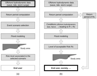
Fig. 1. Principle of direct (a) and inverse (b) approaches. The thick boxes indicate the main input of the approach.
question being: what should be the threshold at the coast and for which elements?
Such an approach has been, for instance, developed within the context of climate change, with the adaptation tipping points (ATP) method developed for flood risk. This method describes the extent to which the climate should change be-fore current flood risk management is no longer efficient (Kwadijk et al., 2010). In such climate change contexts, whereas the traditional top-down approach answers the ques-tion: “what happens if such a climate change scenario oc-curs?”, the ATP approach aims at answering “how much cli-mate change and sea level rise can the current strategy cope with?”. In hydrology, Cunderlik and Simonovic (2007) de-veloped an inverse-type approach aiming at identifying the meteorological conditions leading to critical hydrological ex-posures. However, Cunderlik and Simonovic (2007) consider fewer physical dimensions in their model than in coastal sys-tems because they only included meteorological precipita-tions as forcing condiprecipita-tions. For risk management for other perils inverse approaches are being developed. For example, Douglas et al. (2013) present a French national map for use within seismic building codes derived by targeting a certain level of acceptable risk of structural collapse, rather than a hazard level with a certain return period.
As a first step toward the development of a full inverse method starting from acceptability thresholds, the present paper focuses on the development of an inverse method accounting for the complexity of the relationship between
forcing conditions and water level at the coast, and its appli-cation for an idealised, but one based on real data, test site. In the next section, we describe the principles for the inverse approach. Then, the application to a test site, located on the French Mediterranean coast, is presented. The potential ap-plications, advantages and limitations of the inverse method-ology are subsequently discussed, with a focus on how the present method could trigger participation of stakeholders (limitations L1 – societal needs and limitations L2 – stake-holders involvement). Then, conclusions outlying key issues for future research are drawn.
2 Inverse method: principles, setup and development
2.1 Principles
Figure 1 illustrates, by comparison with a more direct ap-proach (“event-based”), what could be an inverse (“hazard– based”) approach. This schematic representation shows that the input of the “direct” approach is the definition of the scenarios of offshore conditions (Fig. 1), whereas the input of the inverse approach is a hazard threshold. The proposed methodology is based on four main steps.
– Step 0: identify the hazard threshold. This step is
(public). The determination of this input is discussed in Sect. 4.
– Step 1: identify all the offshore conditions leading to
a hazard level larger than the thresholdRC(inversion step). This consists in estimating the boundary of the set of all scenarios of offshore conditions, which lead to
RC(named “critical” frontier). Note that in the present study,RCis the threshold of water level at the coast, in-tegrating storm surge, tide and wave set-up. This step al-ready provides useful information for flood early warn-ing systems.
– Step 2: estimate the return period of these offshore
con-ditions (exceedance probability), i.e. the probability of exceeding the “critical” frontier.
– Step 3: feed-back with stakeholders and support
deci-sion making for coastal risk management using the in-formation on the exceedance probability of the “criti-cal” flooding. This is further discussed in Sect. 4. The description here focuses on steps 1 and 2, considering step 0 as an input for the method. Issues related to steps 0 and 3 are discussed in Sect. 4.
2.2 Inversion
The objective of this step is to estimate the set of offshore conditions that can lead to the hazard thresholdRC. This is achieved through inversion of the model used for hazard as-sessment. For clarity, let us formally defineF as the model used for hazard assessment so thatY=F (X)=f (x1,x2,. . . ,
xN)whereY represents the calculated hazard level andX represents the vector of the forcing conditionsxi (i=1 to
N ), which could be, like in the present study, the offshore water level (ξe)and the wave height (HS). Given a hazard level RC, the first step of the “inverse method” consists in calculating the critical frontier of the setSof offshore forcing conditionsX(j )so thatF (X(j ))≥RC. This formal problem does not have a unique solution and is referred to as the “in-verse problem of the contourRC”. This issue has an analogy with system reliability analysis, which implies estimating the failure probability of a system by integrating over the failure region defined by a contour (also named a “limit state”); see, for example, Haldar and Mahadevan (2000) for further de-tails of reliability analysis. To solve this contour inversion problem, two strategies using directlyF can be proposed de-pending on their computation times.
When the modelF is not expensive to evaluate, the “in-verse problem” can merely be solved in a forward manner consisting in the systematic direct evaluation of the modelF
using a regular grid in the forcing conditions space. To illus-trate, let us consider a regular grid designed for 30 configu-rations ofξe varying by a constant increment step between 0.25 and 1.50 m and 30 configurations ofHS by a constant
increment step varying between 0.5 and 7 m. In two dimen-sions, the desired contour can then be extracted using, for instance, Matlab’s©function contourc, the accuracy of the solution being dependent on the grid increment, hence on the grid size.
Such an approach may, however, become rapidly pro-hibitive when using computational, time-consuming models (with run times varying from hours to days). This issue has given rise to numerous studies either relying on appropriate grid computing architecture (e.g. Boulahya et al., 2007) or on the use of meta-models (also named response surfaces or sur-rogate models). The latter technique consists in replacing the true modelF by a mathematical approximation that predicts the model responses with a negligible computation time cost. In the coastal domain, the application of the meta-modelling approach to the specific case of contour estimation of compu-tationally intensive numerical codes is illustrated by Rohmer and Idier (2012), but it still remains a matter of continuing research.
2.3 Estimation of the return period
The inverse modelling discussed above provides the setSof combinations (ξe;HS)leading to a water level at the coast higher than the maximum acceptable level, i.e. a water level at the coastξecsuch thatξec≥RC. The next step is to com-pute the return periodTRof this setS, also called the annual exceedance probability (1/TR). To compute that return pe-riod, there is a need for a long enough time series ofξe and
HS. This time series can either come from in-situ measure-ments or from model outputs.
The offshore wave height and water level are generally not completely independent since a storm will both generate both a storm surge (increase in the water level) and higher waves (Hawkes et al., 2002; HR Wallingford, 2000a). Thus, a relevant approach is to take into account the dependency between these two hydrodynamic components. For that, the method of joint probability analysis can be used. By defi-nition, this method computes the probability of occurrence of events in which two or more partially dependent vari-ables simultaneously exceed given values. A joint probabil-ity analysis software package for coastal applications named JOIN-SEA was developed during a Defra-funded research programme (Hawkes et al., 2002). Details of the theory, de-velopment, testing and validation of JOIN-SEA are given in (HR Wallingford, 2000a, b). There are five main stages in the analysis:
i. preparation of input data consisting of independent combinations (ξe;HS). These combinations are simul-taneous observations of the two variables at the offshore analysis point (before the breaking of waves);
Mediterranean Sea Lagoon DEMO city
MIR 1 MIR 2
Lido
(a) (b)
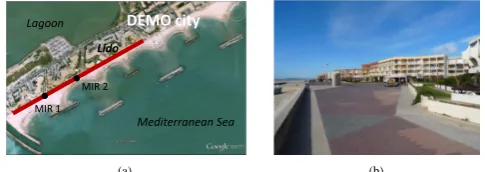
Fig. 2. Site (DEMO City) location with the sea wall position (red line) and observation points (MIR1 and 2) where the inversion cal-culation is performed (a) and photo of the sea wall from point MIR 2 (b).
iii. fitting of a statistical model of dependence betweenξe andHS;
iv. long-term simulation using a Monte-Carlo process gen-erating millions of combinations (ξe;HS)that have the same statistical characteristics as the original data; v. analysis of joint exceedance extremes. It provides
iso-joint exceedance return period points in the variable space (ξe; HS): for each point (x, y) on one of these iso-return period contours, the probability of the event
{ξe> x, HS> y}is such that this event occurs on
aver-age once during the return period.
In our specific study, we are interested in the return period of
S (see Fig. 8, red area), not on any joint exceedance return period of bothξeandHS(see Fig. 8, green area). Therefore, once stage (iv) has been performed, the return period ofSis calculated using the following formula:
RP (S)= 1
E×Pr(S) (1)
with Pr the probability of exceedance ofSsuch that Pr(S)= 1
N N
P
i=1
1X∈S(Xi).E is the number of observations per year,
N is the number of simulated combinations,Xrepresents a couple (ξe;HS), and 1X∈Sis the indicator function ofS, such that ifXi∈S, 1X∈S(Xi)=1, otherwise=0.
3 Application
3.1 Study site and hazard threshold
In this study the site application is based on a real case, but the results are mainly for demonstration purposes. Further-more, the method is applied for strategic planning, such that it accounts for small impact–high frequency events, and such that the hazard threshold is defined as the maximum accept-able hazard level. The presented results are not to be inter-preted as a definitive risk assessment. That is why we choose to use a fictive city name. In the present case, the study site
50 cm
lake sea
Wave breaking area Swan computations
Offshore conditions
(xe, Hs) Rc
Fig. 3. Cross-shore scheme of the study case.
is a city, which we called DEMO in this demonstration exer-cise, lying on a lido protecting the lagoon.
This site is located on the Mediterranean coast (Fig. 2). A regional study (Vinchon et al., 2008) identified that the lido is a regional “hot-spot”. DEMO is characterised by significant touristic activities. At the sea-front, there are pedestrian ar-eas, which have already been flooded in, at least, two storms: 6–8 November 1982 and 4 December 2003. This pedestrian area is limited by a sea wall having a height of about 50 cm above the pavement (Fig. 3) but with some openings.
0 5 10 15 20 25
0.0 0.2 0.4 1.0 2.5 5.0 10.0 100.0
%
of
ans
w
er
s
Return period of unaceptability of sea‐flood for which people are moving
(year)
Fig. 4. Threshold of acceptability to sea flooding, based on the an-swers of residents and shopkeepers of DEMO city to the question: Above which frequency of sea-flooding inundation of your house, would you leave your home? The results exclude the 5.5 % who did not answer. Data provided by the MISEEVA project (Vinchon et al., 2010).
of 6.5 yr. This value is used henceforth. This value implies that DEMO city should not be flooded more than once ev-ery 6.5 yr on average and means that 70 % of the intervie-wees would move in case it is flooded more than once every 6.5 yr (Fig. 4). Such proportion would have significant con-sequences on the local activities. We make the assumption that this critical flooding return period means it is intolera-ble that water enters the area through the sea wall openings more than once every 6.5 yr, and specifically at points MIR1 and MIR2 (Fig. 2) which are just in front of connection roads with the lagoon.
It is worth noting that the level of what is tolerable or not depends also on the risk culture and the perception of dan-ger. In the present demonstration, we assume that the main concerns of the society are to preserve economical activities and tourism of the DEMO city, which contributes to a large extent to the image and the attractiveness of the region. Obvi-ously, for another site or for another type of application (e.g. early warning or emergency management), the level might be different. For example, it might correspond to a critical impact such that fatalities are intolerable. Then, the hazard level (RC)might be such that the water level does not reach the first storey of buildings.
3.2 Inversion
3.2.1 Model to inverse
For sake of clarity, we assume that the flooding of the lido is not influenced by the lagoon, and we also neglect the influ-ence of the lido on the submersion phenomenon. First, we remind the reader that the water level at the coast ξec re-sults from the offshore water levelξe (tide and meteorolog-ical storm surge) and the run-up resulting from two dynam-ical processes, which are the wave set-up ηand the swash
S. Here, we set a modelling strategy to account for these three contributions (ξe; η; S). For the offshore water level contribution, we assume that ξe induced by storm surges
Fig. 5. 2-D domain of the SWAN implantation used for the inver-sion.
and tide is uniform in the local area. For the set-up and run-up induced by waves, we need a more sophisticated ap-proach. First, the wave set-upηis computed using the code SWAN (Booij et al., 1999). It solves the wave action equa-tion and provides wave spectra and wave set-up. At the off-shore boundary, uniform sea level and wave height are im-posed. The bathymetric and topographic data used here have been obtained through lidar measurements (data provided by DREAL LR), as well as bathymetric surveys (data provided by SHOM). The grid size is 2 m (Fig. 5). Second, to com-pute the swash-induced elevationS, we use the formulation of Stockdon et al. (2006). Based on the assumption of reflec-tive beach, the analysis of the equations proposed in Stock-don et al. (2006) shows that we can, as a first approximation, assume thatSis equal to the set-up. Thus the total maximum water levelξecat the beach is calculated as follows:
ξec=ξe+2η. (2)
The inversion is based on this model (SWAN and the swash formula of Stockdon et al., 2006).
3.2.2 Inversion results
We inverse the system to provide offshore conditions in the variable space (ξe;HS). The wave period and the wave direc-tion are fixed at their most frequently observed values. For the present case, the analysis of a few years’ worth of wave data from a buoy located in the south-east of the area indi-cates that the dominant wave incidence angle is 105◦
(corre-sponding to a nautical wave direction of 135◦N), for a wave period of 7 s. Thus, the return period of the combination (ξe;
HS)is computed for a wave dataset restricted to this fixed wave period and direction.
ξe (m)
Hs
(m
)
Point MIR 1
0.5 1 1.5
1 2 3 4 5 6 7
ξe (m)
Hs
(m
)
Point MIR 2
0.5 1 1.5
1 2 3 4 5 6 7
2.3 2.45 2.6
2.15
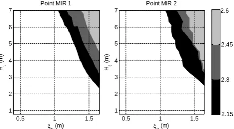
Fig. 6. Total water levelξec(m) at the beach versus offshore water levelξeand offshore significant wave heightHS.
and simulated 30×30 different configurations of the offshore forcing conditions (ξe;HS)using a cluster of ten computer units, which enables the overall computation to take less than one day. The results at the MIR1 and MIR2 locations (Fig. 6) indicate there is a range of couples (ξe;HS)such that the threshold value of the total water level at the beach is ex-ceeded. For instance, at point MIR1, for an offshore water level of 1.5 m (compared to the vertical IGN reference), an offshore significant wave height of 6 m would induce a total local water level exceeding the critical value and thus leading to water entering through the wall openings.
3.3 Return period of the hazard threshold
3.3.1 Offshore time series generation
Ideally, the inversion step would provide water levels and wave heights at a location where continuous measurements are made (permanent buoys or sensors). In some places, this is indeed the case. In the present study, there are no obser-vations of water levels or wave conditions at the selected site. Thus, there is a need to find a time series dataset, cor-responding to the conditions at the offshore boundaries of the SWAN implementation (Fig. 5). For this purpose, we use numerical model outputs. Concerning the waves, outputs of the WW3 model, implemented in this area by Ardhuin et al. (2010), are used. The closest node of the WW3-grid having the same water depth as the offshore boundary of the SWAN model is used. This point is located 1 km south-west of the DEMO site. The quality of the WW3 implementation in Mediterranean Sea has been investigated by Ardhuin et al. (2007) who show that the best fit slope between the mod-elled and observed wave heights is about 0.84–0.87 for the WW3 model forced by ALADIN wind data (M´et´eo-France). Thus, for the demonstration, we corrected the WW3 outputs to compensate for this error, by multiplying the significant wave height by a factor of 1.18 (i.e. 1/0.85).
Furthermore, for the water level, numerical computations are performed using the MARS2DH model (Lazure and
10-1 100 101 102
1.1 1.2 1.3 1.4 1.5 1.6 1.7
Return period (years)
ξe
(m
)
Data (Hazen) GPD ML
68% confidence interval 95% confidence interval
Fig. 7. Best fit of the GPD model and confidence intervals for the marginal distribution ofξe. Parameters of the GPD calculated with the method of maximum likelihood. Threshold: 1.19 m.
Dumas, 2008). The background of the implementation of the MARS2DH model for the study area as well as its valida-tion is presented in Pedreros et al. (2011). Here, the simula-tions are based on FES2004 (Lyard et al., 2006) for the tidal boundary conditions and on the Climate Forecast System Re-analysis (CFSR, Saha et al., 2010) for wind and pressure.
Finally, a sea level dataset of 13 yr and a wave dataset of 5 yr are provided.
3.3.2 Return period ofR≥RC
The preparation of input data (selection of independent events) for the joint probability analysis was performed in two stages. First, one event per day was selected taking the daily maximum of HS with a minimum 12 h duration be-tween two successive events. Then, to each of these HS peaks, the maximum ofξein a temporal window of 12 h cen-tred on the peak ofHSwere associated. This is a conservative approach that allows capturing the highest values of the wa-ter level signal. In all, 231 events per year were selected in this way.
For the calculation of marginal distribution ofξe, instead of using the default JOIN-SEA distribution that is based on waves and water levels data covering the same temporal pe-riod (i.e. 5 yr), we fitted a new GPD forξe using all avail-able data (13 yr). The parameters were calculated using the method of maximum likelihood. The threshold choice was selected using several techniques (based on visual apprecia-tion of quantile–quantile plots, residual life plot, and statis-tical tests Chi2, Kolmogorov–Smirnov and so forth; see, e.g. Coles, 2001). A threshold of 1.19 m was considered as pro-ducing the best fit (Fig. 7).
The statistical model for dependence between ξe and
HS is a mixture of two bivariate normal distributions (HR Wallingford, 2000a). This model is fitted to the data after conversion of the variables to normal scales.
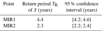
Table 1. Return period ofS(combinations that lead to exceedance ofRC)and 95 % confidence interval for both study points.
Point Return periodTR 95 % confidence ofS(years) interval (years)
MIR1 4.4 [4.2;4.6]
MIR2 2.3 [2.2;2.4]
2 310 000 combinations (ξe;HS). The last stage of the anal-ysis leads to estimation of the curves of iso-joint exceedance return period (black curves on Fig. 8). Using the limit pro-vided in the inversion step (red line on Fig. 8) and Eq. (1), allows estimation of the return period of setS or, in other words, the probability of exceedance of the critical water level at the coastRC, for points MIR1 and 2. Figure 8 illus-trates the result for point MIR1. This exercise leads to a re-turn period ofR(=ξec)≥RCcomprised between 2.3 (point MIR2) and 4.4 yr (point MIR1) (Table 1).
Table 1 and Fig. 6 show the spatial heterogeneity of the return period ofR≥RCalong the coast, with point MIR2 having, for instance, almost twice the chance to encounter a sea level exceeding the critical value than point MIR1.
3.4 Use for coastal risk management
The return periods at points MIR1 (4.4 yr) and MIR2 (2.3 yr) are smaller than the acceptable one (TRC=6.5 yr). In the light of this result, the acceptability threshold of 6.5 yr should be re-discussed (with decision-makers, stakeholders and populations). This iteration has three main purposes. First, one aim is to increase the stakeholder’s awareness of risks. Indeed, as illustrated by Kievik and Guttelling (2011), a certain level of risk awareness is required to encourage the public to adopt self-protective behaviour. A second purpose is to help and encourage them to hierarchize their priorities in terms of coastal planning and management. This prioriti-sation can be done based, for instance, on multi-criteria de-cision making (Karlsson, 1996) or group consensus methods (Gervais and Pepin, 2002). Lastly, one is to help the decision makers weigh up the different risk management actions, for instance strengthen the coastal defences (but at what cost?), invest in flood-proofing of buildings, or improve warning systems (DELTARES, 2010).
More particularly, two possible outcomes of this feedback can be envisaged. The first one is if it is decided that the ac-ceptable return period of the hazard threshold remains at the original value of 6.5 yr, coastal risk management should then focus on preventive actions at the level of the city defences (e.g. increase in control of dikes: maintenance; reinforce-ment when required; “build with nature”, like flood protec-tion by beach nourishment; Delta Committee, 2008) or at the planning level (e.g. urban development). A second possible outcome of the feedback process is to accept a shorter return period than 6.5 yr (e.g. 2 yr), but under the condition that an
Fig. 8. Illustration of the results for point MIR1. The original data points (independent events) are represented by yellow dots while simulated combinations are represented by blue dots. The black curves represent the contours of iso-joint exceedance return period. The red curve is the limit ofS(combinations that lead to exceedance ofRC)which is represented by red dots. The joint exceedance do-main for the combinationWwhich represents the worst case ofS
is pictured in green (i.e. the combination whose joint exceedance return period is the lowest).
early warning system is set up allowing for minimisation of the economic, environmental and human cost of flooding.
4 Discussion
The initial development of the inverse approach had two main objectives: improve hazard assessment; and improve awareness and preparedness, preparedness being defined as the “knowledge and capacities developed by governments, professional response and recovery organisations, communi-ties and individuals to effectively anticipate, respond to, and recover from the impacts of likely, imminent or current haz-ard events or conditions” (UNISDR, 2009). How the method contributes to these two objectives is discussed here.
4.1 Hazard assessment
4.1.1 A “decoupled-strategy”
From a physical point of view, as stated before, traditional (direct) approaches used to build coastal flooding maps are based on offshore scenarios propagated to the coast (event-based approach), which can present strong limitations (de-noted L3, as described in the introduction).
In the present study, we estimated the return period of a total water level exceedingRC at point MIR1 as 4.4 yr. A scenario-based approach on point MIR1 would have proba-bly induced the selection of the combination represented by point W on Fig. 8, which corresponds to the worst case ofS
characterised byR≥RC. This factor of two has already been identified in the literature (Hawkes et al., 2002; Garrity et al., 2006). This illustrates that selecting a scenario, based on the choice of an offshore couple having a joint exceedance re-turn period ofT years, will likely lead to a hazard map of a return period possibly closer toT /2 years than toT years. Furthermore, as mentioned by Jonkman et al. (2008) in a study of flood risk in South Holland, in future analyses spe-cial attention should be given to more extreme flood scenario than the ones they studied, because unlikely extreme scenar-ios already happened in the past (e.g. Katrina induced flood-ing in 2005). In principle, the proposed inverse method could be a way to better identify the likelihood of some unlikely extreme hazard level at the coast. Thus, the inverse method we propose limits the bias induced by the a priori selection of a specific event scenario and accurately computes the re-turn period of hazard being larger or equal to the critical one (exceedance), as the “Response” methods (see Garrity et al., 2006). This allows overcoming limitation L3.
Moreover, the present method further improves the “Re-sponse” methods thanks to its decoupling of the differ-ent phases: (1) a first step consists in estimating all the forcing offshore conditions so that the water level at the coast exceeds the maximum acceptable levelRC (step 1); (2) a second step uses the set of offshore conditions (i.e. a critical frontier defined in the domain of offshore con-ditions) to compute the return period associated with the event “exceedingRC” by means of a statistical analysis of extremes and of a Monte-Carlo-based approach (step 2). Such an approach allows computation of the critical fron-tier in a deterministic fashion, i.e. independently from any notion of probability. This presents several advan-tages. First, this allows an in-depth exploration of the do-main of offshore conditions to identify the critical fron-tier, either using a grid-based approach as used here for the test case or a more advanced method using a meta-modelling technique (Rohmer and Idier, 2012). Such con-tour information can be useful, for instance, in forecasting systems (e.g. PREVIMER – http://www.previmer.org, NIV-MAR – http://www.puertos.es/oceanografia y meteorologia/ redes de medida/index.html), early warning systems (Harley et al., 2012; Ciavola et al., 2011; Norbiato et al., 2008; Safe-coast, 2008), or coastal observatories (such as the Chan-nel Coastal Observatory, http://www.chanChan-nelcoast.org). Sec-ondly, this makes the step involving statistical analysis of extremes independent, which can be of great interest when the return-period calculation has to be updated by integrat-ing, for instance, scenarios of climate change. The advan-tage of this “de-coupled strategy” is illustrated in the inverse approach developed by Cunderlik and Simonovic (2007), which aims at better integrating changing climatic conditions in flood-risk modelling. Thus, even if climate and offshore conditions are changing, the method does not require the whole procedure to be repeated (contrary to the “response” method), but only to repeat step 2.
4.1.2 Uncertainties in inversion and exceedance return period
Within the inversion step, several uncertainties can be iden-tified. First, the model by itself contains uncertainties. To reduce it, the first step is to choose the model in accor-dance to the flooding regime (direct inundation, overtopping, breaching) associated with the selected threshold: a very high threshold of water level at the coast for instance implies a direct inundation, whereas a threshold just above coastal de-fense height implies mainly overtopping processes. For a di-rect inundation regime, several approaches could be used, ne-glecting overtopping, like for instance the “bathtub” method (e.g. based on hydrodynamic model providing water level at the coast, the water level being projected inland using GIS) or full 2-DH modelling (Hervouet and van Haren, 1993). For the overtopping regime, other approaches are required, either integrating overtopping calculation formulae, or describing the full dynamics using Boussinesq-type models (Cheung et al., 2003; Wadey et al., 2012; Chini et al., 2013). In this paper, the model we used was simple, designed for demon-stration purposes. The use of the most sophisticated models (fully nonlinear weakly dispersive models, like the one devel-oped by Bonneton et al., 2011) would allow for a reduction in the model uncertainties used for the inversion, but may require more sophisticated approaches for the inversion, as discussed in Sect. 2.2. For instance, Rohmer and Idier (2012) developed a strategy based on the kriging meta-modelling technique combined with an adaptive sampling procedure aimed at improving local accuracy in the regions of the off-shore conditions that contribute most to the estimate of the targeted contour (threshold). They show that the critical off-shore conditions can be accurately estimated using a limited number (a few tens) of computationally intensive hydrody-namic simulations.
the inversion procedure remains a matter of ongoing re-search. The recent advances in optimisation of stochastic functions (Picheny et al., 2013) could be a starting point for such investigations.
Finally, the offshore dataset quality can influence the re-sults on exceedance return period. In the present study, it has been constructed using a modelling approach. Thus, there are some uncertainties in the values that have been used. This source of uncertainty would vanish for locations where wave data buoys and tide gauges are available. This illus-trates that the present approach would be especially useful where hydrodynamic data exist offshore the site of interest. Hence, there is a need for hydrodynamic data monitoring in the vicinity of the identified vulnerable sites, in addition to operational models.
4.2 Coastal risk management, awareness and preparedness
The second objective of the inverse approach is to improve the authorities and society “awareness and preparedness”, by raising the question of risk acceptability and by triggering stakeholders’ participation.
One of the potential advantages of the proposed inverse approach is that the final result is a return period of a hazard level identified as the threshold above which such a hazard is intolerable. A comparison of that return period with the one considered previously as acceptable should raise awareness of the actual risk. Thus, in the inverse approach, the input determination (hazard threshold) should be associated with a “realistic” point of view of the acceptable likelihood of the threshold being exceeded.
As an indirect advantage, the proposed method would al-low reliance on a strong implication of the stakeholders (e.g. society and decision-makers). This transfer of knowledge should be useful not only for territorial planning, but also for preparedness and emergency purposes. This seeks to over-come limitation L1 (as described in the introduction).
The present inverse method requires the identification of a hazard threshold (RC)for the input. The way this threshold is defined and the nature of this threshold depend on the needs of the stakeholders. Furthermore, this threshold has to be identified in collaboration with stakeholders to ensure both substantive (integration of stakeholders’ knowledge) and in-strumental (trust of stakeholders) rationale (Meyer et al., 2012). As highlighted in the introduction, the determination of hazard threshold raises the question of risk acceptability. A detailed discussion of risk acceptability is beyond the scope of this article. Nevertheless, we discuss what would be the benefit of the inverse method within risk evaluations based on acceptability. A widely used tool for displaying risk is the frequency/impact (also named frequency/consequence) graph (e.g. Ballard, 1993), as schematically depicted in Fig. 9. On this basis, the critical limit between what is ac-ceptable or not can be defined. This limit can either be small
Fig. 9. Risks areas: normal, intermediate and intolerable. Adapted from Farmer (1967). Three cases are depicted. Risk event A: low impact/high probability of occurrence; Risk event B: intermediate case; Risk event C: high impact/low probability of occurrence cor-responding to a catastrophic event.
impact/high probability (point A), or high impact/low prob-ability (C), and both could be “intolerable” for the society. In the case of flooding, Haimes (2004) found that people are “often more concerned with low probability catastrophic events than with more frequently occurring but less severe accidents”. As stated by Renn (2008a), investigation of the perception of rare but possible catastrophic events shows that probability hardly plays any role. In other cases, for smaller impact events, society accepts that they happen up to a crit-ical occurrence probability (or return period), above which they cannot be tolerated or afforded anymore (Renn, 2008a). Even if there are some differences, one of the most consistent findings within and across cultures is that usually the same concepts (e.g. dread and unknown risks) emerge, but receiv-ing different priorities (Kasperson, 1986), leadreceiv-ing to different levels of risk acceptance. In principle, the inverse approach would allow these to be taken into account in various con-texts, with difficulty remaining in reaching a consensus in the definition of the acceptability thresholds.
criteria to analyse how the estimated flood risks (probabil-ity of fatalities) in South Holland compare with the accept-able flood risk. Such criteria also allow for the comparison with other societal risks (e.g. chemical and aviation). In the Netherlands, such acceptability criteria are appropriate be-cause a large part of the country is under sea level; therefore, flood risks are highly related to the height of dikes and their standards and resistance. However, in other places, such cri-teria based on fatalities do not exist with respect to flood risk. For instance, regarding flood early warning systems for rivers in France, thresholds of no, low, medium and high levels of alerts are mainly based on empirical and historical knowl-edge (for such water levels, a certain damage level occurred in the past), rather than on fatalities or damage probabilities. Thus, one potential utility of the inverse approach would be to be flexible enough to adapt to the various criteria of ac-ceptability that could exist.
Identifying in practice what is acceptable and getting a consensus of stakeholders raises the question of governance, i.e. the coordination of stakeholders, social groups, and insti-tutions to reach a common objective in fragmented and un-certain environments (Bagnasco and Le Gal´es, 1998). First, it should be noted that flood governance and policy in Europe are changing. The role of the state and individual responsibil-ity for risk management are now key contemporary issues in European flood policy, as highlighted by the 2007/60/EC EU Directive. This policy aims at enhancing the responsibilities of local authorities in flood risk management and reducing the role of national governments, such that local authorities have now to lead partnerships with local stakeholders to en-sure effective flood risk management. One of the challenges within the development of a full inverse method is then how to get a consensus between the stakeholders regarding risk acceptability. Some methods have been developed to cope with uncertainty in a complex world (Renn, 2008c) but also to deal with the issue of stakeholders consensus, like the correlation method (Ahmad, 2008), multi-criteria methods like the analytical hierarchy process (Karlsson, 1996), cost-benefit methods (Hermann and Daneva, 2008) and group dis-cussion like the TRIAGE method (Gervais and Pepin, 2002).
5 Conclusions, recommendations, perspective
The societal significance of a risk and its acceptance not only depends on its physical dimension, but also on its societal perception, which is inherently a context-dependent process and is affected by social, political, cultural and economic factors as recently outlined by the FP7 CapHaz-Net project (Wachinger and Renn, 2010). Thus, in order to ensure an ap-propriate response for the decision makers, there is a need to develop flexible risk assessment methods regarding the end user needs and triggering their participation.
Knowledge of risk requires estimates of the return period (or exceedance probability) of critical levels of hazard. The
proposed methodology intends to achieve the objective of es-timating the return period of a given hazard threshold. As-suming that the hazard threshold (RC) is known, the two main steps of the methods have been identified: offshore con-ditions identification (step 1) and assessment of physical re-turn period (or exceedance probability)TR(step 2). Assum-ing a critical impact and a plausible level of acceptability, the practicability of steps 1 and 2 is demonstrated using a real case application from southern France.
The inverse method has been proposed as a method that could contribute to raise the risk acceptability question, to provide data for early warning systems, and to trigger stake-holder participation, to improve their awareness and pre-paredness to potential floods. This article investigated the first development stage of the method. At this stage, several recommendations can be made, based on this preliminary de-velopment:
– Provided that a critical asset has been identified
(hos-pital, energy plant, etc.) and that the associated maxi-mum “acceptable” inundation height has been defined, the aforedescribed methodology (step 1 and 2) can be implemented to estimate the return period of exceeding the identified maximum “acceptable” inundation height, for this localised sector. Furthermore, this could be used for localised risk assessment. It can also be used to iden-tify extreme scenarios that were previously thought not possible, like for instance the Xynthia event (Bertin et al., 2012). This type of application falls in the field of stress test design (as it has been developed, for instance, for nuclear plants after the Fukushima earthquake by the West European Nuclear Regulators Association, 2011).
– For early warning systems, the method (step 1) could
be used to trigger various levels of alerts. For instance, several critical water levels at the coast can be identi-fied: class 1 (water level reaching the safety minimum altitude of the coastZc, so that for suchZc, the water level at the coast is just at the limit of flooding), class 2 (water level reaching 1 m aboveZc), class 3 (water level 2 m aboveZc) and so forth. The inverse method can be used to identify the offshore combinations lead-ing to these classes, such that early warnlead-ing systems can provide information on water level at the coast, without necessarily running a refined but computationally inten-sive model every day.
– The final result of the inverse method is the return
What is the return period? Is it different from the one perceived as the “maximum acceptable”? If so, what ac-tions can be undertaken?). Step 1 and 2 of the present method can support these territorial tests.
The proposed inverse method is expected to have strong implications in terms of decision making for coastal risk management. Yet, so that the inverse method fulfils its role in addressing the limitations identified in the introduction (L1-3), a necessary, but challenging next step is to fully address the issue of risk and hazard acceptability. To reach this objec-tive, a possible research line would be vulnerability analysis enabling identification of critical asset(s) and associated crit-ical impact(s) (e.g. asset damage and failure of the asset func-tion), taking into account lifelines (i.e. physical or virtual net-works that are vital to health, safety, comfort and economic activity, see, e.g. Platt, 1995) and dependence (i.e. everything an asset depends on, see, e.g. D’Ercole and Metzger, 2009). Such vulnerability analysis, independent of scenario and haz-ards, could also be useful for multi-risk analysis.
Acknowledgements. The authors thank the ANR VMC 2006 project VULSACO no. ANR-06-VULN-009, the ANR VMC 2007 project MISEEVA no. ANR-07-VULN-007 as well as the BRGM-funded VULNERISK project, for contributions to the financial support of the present work. A. Magnan, M. Poumad`ere, M. Garcin, C. Oliveros, E. Foerster and A. L. Gautier are acknowledged for fruitful discussions and support. The authors are also grateful to R. Pedreros, V. Turpin and C. Vinchon for their contribution, and to P. Hawkes, resp. Ifremer, for providing the JOIN-SEA, resp. MARS2DH, software. The MISEEVA team working on the public flooding risk representation (specifically C. Meur-Ferec, B. Rulleau, H. Rey-Valette, and their team) is also acknowledged for providing the results of their survey. The authors like also to thank J. Douglas for checking the English. Lastly, J. Beckers, O. Renn and the anonymous reviewer are acknowledged for their constructive comments.
Edited by: O. Katz
Reviewed by: J. Beckers, O. Renn, and one anonymous referee
References
Ahmad, S.: Negotiation in the Requirements Elicitation and Analy-sis Process, IEEE, ISBN: 978-0-7695-3100-7, 683–689, 2008. Ardhuin, F., Bertotti, L., Bidlot, J. R., Cavaleri, L., Filipetto, V.,
Lefevre, J. M., and Wittmanne, P.: Comparison of wind and wave measurements and models in the Western Mediterranean Sea, Ocean Eng., 34, 526–54, 2007.
Ardhuin, F., Rogers, E., Babanin, A. V., Filipot, J. F., Magne, R., Roland, A., van der Westhuysen, A., Queffeulou, P., Lefevre, J. M., Aouf, L., and Collard, F.: Semi-empirical Dissipation Source Functions for Ocean Waves, Part I: Definition, Calibration, and Validation, J. Phys. Oceanogr., 40, doi:10.1175/2010JPO4324.1, 2010.
Bagnasco, A. and Le Gal`es, P.: Villes en Europe, Revue franc¸aise de sociologie, 39-4, 808–810, 1998.
Ballard, G.: Guest editorial: societal risk-progress since Farmer, Re-liability Eng. Syst. Safe., 39, 123–127, 1993.
Bertin, X., Bruneau, N., Breilh, J. F., Fortunato, A., and Karpytchev, M.: Importance of wave age and resonance in storm surges : the case of Xynthia, Ocean Modell., 42, 16–30, 2012.
Bonneton, P., Barthelemy, E., Chazel, F., Cienfuegos, R., Lannes, D., Marche, F., and Tissier, M.: Recent advances in Serre–Green Naghdi modelling for wave transformation, breaking and runup processes, Eur. J. Mech. B.-Fluid, 30, 589–597, 2011.
Booij, N., Ris, R. C., and Holthuijsen, L. H.: A third-generation wave model for coastal regions, Part I: Model description and validation, J. Geophys. Res., 104, 7649–7666, 1999.
Bottelberghs, P. H.: Risk analysis and safety policy developments in the Netherlands, J. Hazardous Materials, 71, 59–84, 2000. Boulahya, F., Dubus, I. G., Dupros, F., and Lombard, P.:
Foot-print@work, a computing framework for large scale paramet-ric simulations: application to pesticide risk assessment and management, in: Forum EGEE Enabling Grids for E-sciencE, Manchester, UK, 160 pp., 2007.
Cheung, K. F., Phadke, A. C., Wei, Y., Rojas, R., Douyere, Y. J. M., Martino, C. D., Houston, S. H., Liu, P. L. F., Lynett, P. J., Dodd, N., Liao, S., and Nakazaki, E.: Modeling of storm-induced coastal flooding for emergency management, Ocean Eng., 30, 1353–1386, 2003.
Chini, N. and Stansby, P.: Extreme values of coastal wave overtop-ping accounting for sea level rise and climate change, Coastal Eng., 65, 27–37, doi:10.1016/j.coastaleng.2012.02.009, 2012. Chini, N., Stansby, P., Rogers, B. D., Vacondio, R., and Mignosa,
P.: State-of-the-art coastal inundation models applied to the 2007 Norfolk storm. FLOODRisk conference 2012, in: Comprehen-sive Flood Risk Management, edited by: Klijn, F. and Schweck-endiek, T., Taylor & Francis Group, London, ISN 978-0-415-62144-1, 501–508, 2013.
Ciavola, P., Ferreira, O., Haerens, P., Van Koningsveld, M., and Armaroli, C.: Storm impacts along European coastlines, Part 2: lessons learned from the MICORE project, Environ. Sci. Policy, 14, 924–933, 2011.
Coles, S.: An introduction to Statistical Modelling of Extreme Val-ues, London, Springer Series in Statistics, 2001.
COMRISK: Subproject 1 – Evaluation of policies and strategies for coastal risk management, Directorate-General of Public Works and Water Management – National Institute for Coastal and Ma-rine Management/RIKZ, 2004.
Cunderlik, J. M. and Simonovic, S. P.: Inverse flood risk modelling under changing climatic conditions, Hydrol. Process., 21, 563– 577, 2007.
Deboudt, P.: Towards coastal risk management in France, Ocean Coast. Manage., 53, 366–378, 2010.
Delta Committee: Working together with Water, Findings of the Deltacommissie, Secretariat Delta committee, the Hague, the Netherlands, available at: http://www.deltacommissie.com/doc/ deltareport full.pdf (last access: 1 March 2012), 2008.
DELTARES: Flood Risk Management, available at: http://www. deltares.nl/xmlpages/TXP/files?p file id=14056 (last access: 3 April 2013), 2010.
cybergeo.revues.org/22022; doi:10.4000/cybergeo.22022, 2009. Divoky, D. and McDougal, W. G.: Response-based coastal flood
analysis, Proc. 30th ICCE, ASCE, 5291–5301, 2006.
Douglas, J., Ulrich, T., and Negulescu, N.: Risk-targeted seismic design maps for mainland France, Nat. Hazards, 65, 1999–2013, doi:10.1007/s11069-012-0460-6, 2013.
EU: Directive 2007/60/EC of the European parliament and of the council of 23 October 2007 on the assessment and management of flood risks, 2007.
Farmer, F. R.: Siting criteria – a new approach, Atom, 128, 152– 179, 1967.
FEMA: Wave runup and overtopping, FEMA Coastal Flood Hazard Analysis and Mapping Guidelines Focused Study Report, 51 pp., 2005.
FEMA: Guidelines and specifications for Flood Hazard Mapping Partners, 2011.
Freeman, E.: The Stakeholder Approach Revisited, Z. Wirtschafts Unternehmensethik, 5, 220–241, 2004.
Gamper, C. D. and Turcanu, C.: Can public participation help man-aging risks from natural hazards?, Safety Sci., 47, 522–528, doi:10.1016/j.ssci.2008.07.005, 2009.
Garrity, N. J., Battalio, R., Hawkes, P. J., and Roupe, D.: Evaluation of the event and response approaches to estimate the 100-year coastal flood for Pacific coast sheltered waters, Proc. 30th ICCE, ASCE, 1651–1663, 2006.
Gerritsen, H.: What happened in 1953? The Big Flood in the Netherlands in retrospect, Phil. Trans. R. Soc. A, 363, 1271– 1291, doi:10.1098/rsta.2005.1568, 2005.
Gervais, M. and P´epin, G.: TRIAGE: a new group technique gain-ing recognition in evaluation, Evaluation J. Australasia, 2, 45–9, 2002.
Haimes, Y. Y.: Risk of Extreme Events and the Fallacy of the Ex-pected Value, in: Risk Modeling, Assessment and Management, edited by: Sage, A. P., John Wiley & Sons, Hoboken, 299–321, 2004.
Haldar, A. and Mahadevan, S.: Probability, reliability, and statistical methods in engineering design, Wiley, New York, 2000. Harley, M., Valentini, A., Armaroli, C., Ciavola, P., Perini, L.,
Cal-abrese, L., and Marucci, F.: An early warning system for the on-line prediction of coastal storm risk on the Italian coastline, Coast. Eng. Proceed., 1, doi:10.9753/icce.v33.management.77, online first, 2012.
Hawkes, P. J., Gouldby, B. P., Tawn, J. A., and Owen, M. W.: The joint probability of waves and water levels in coastal engineering design, J. Hydraul. Res., 40, 241–251, doi:10.1080/00221680209499940, 2002.
Herrmann, A. and Daneva, M.: Requirements Prioritization Based on Benefit and Cost Prediction, 16th IEEE International Require-ments Engineering Conference, doi:10.1109/RE.2008.48, 2008. Hervouet, J.-M. and Van Haren, L.: Recent advances in numerical
methods for fluid flows, in: Floodplain Processes, edited by: An-derson, M. G., Walling, D. E., Bates, P. D., Wiley, Chichester, 183–214, 1996.
HR Wallingford with Lancaster University: The joint probability of waves and water levels: JOIN-SEA: A rigorous but practical new approach, HR Report SR 537, 2000a.
HR Wallingford: The Joint Probability of Waves and Water Levels: JOIN-SEA – Version 1.0, User Manual, Report TR71, 2000b.
Jonkman, S. N., Kok, M., and Vrijlin, J. K.: Flood Risk As-sessment in the Netherlands: A Case Study for Dike Ring South Holland, Risk Anal., 28, 1357–1373, doi:10.1111/j.1539-6924.2008.01103.x, 2008.
Karlsson, J.: Software Requirements Prioritizing, ISBN: 0-8186-7252-8, IEEE, 110–116, 1996.
Kasperson, R. E.: Six Propositions on Public Participation and Their Relevance for Risk Communication, Risk Anal., 6, 275–281, doi:10.1111/j.1539-6924.1986.tb00219.x, 1986.
Kennedy, M. C. and O’Hagan, A.: Bayesian Calibration of Com-puter Models, J. Roy. Stat. Soc., 63, 425–464, 2001.
Kievik, M. and Gutteling, J. M.: Yes, we can: motivate Dutch cit-izens to engage in self-protective behavior with regard to flood risks, Nat. Hazards, 59, 1475–1490, doi:10.1007/s11069-011-9845-1, 2011.
Kirwan, B., Hall, A., and Hopkins A.: Changing regulation – Con-trolling risk in society, Oxford, Pergamon, 2002.
Kwadijk, J. C. J., Haasnoot, M., Mulder, J. P. M., Hoogvliet, M. M. C., Jeuken, A. B. M., van der Krogt, R. A. A., van Oostrom, N. G. C., Schelfhout, H. A., van Velzen, E. H., van Waveren, H., and de Wit, M. J. M.: Using adaptation tipping points to prepare for climate change and sea level rise: a case study in the Netherlands, WIREs Clim Change, 1, 729–740, doi:10.1002/wcc.64, 2010. Lazure, P. and Dumas, F.: An external-internal mode coupling for
a 3D hydrodynamical model for applications at regional scale (MARS), Adv. Water Res., 31, 233–250, 2008.
Lyard, F., Lefevre, F., Letellier, T., and Francis, O.: Modelling the global ocean tides: modern insights from FES2004, Ocean Dy-nam., 56, 394–415, doi:10.1007/s10236-006-0086-x, 2006. Meyer, V., Kuhlicke, C., Luther, J., Fuchs, S., Priest, S., Dorner,
W., Serrhini, K., Pardoe, J., McCarthy, S., Seidel, J., Palka, G., Unnerstall, H., Viavattene, C., and Scheuer, S.: Recommen-dations for the user-specific enhancement of flood maps, Nat. Hazards Earth Syst. Sci., 12, 1701–1716, doi:10.5194/nhess-12-1701-2012, 2012.
Nicholls, R. J., Hanson, S. E., Lowe, J. A., Vaughan, D. A., Lenton, T., Ganopolski, A., Tol, R. S. J., and Vafeidis, A. T.: Improving methodologies to assess the benefits of policies to address sea-level rise, Report to OECD, Paris, 135 pp., 2006.
Norbiato, D., Borga, M., Esposti, S. D., Gaume, E., and Anquetin, S.: Flash flood warning based on rainfall thresholds and soil moisture conditions: An assessment for gauged and ungauged basins, J. Hydrol., 362, 274–290, 2008.
O’Sullivan, J. J., Bradford, R. A., Bonaiuto, M., De Dominicis, S., Rotko, P., Aaltonen, J., Waylen, K., and Langan, S. J.: Enhanc-ing flood resilience through improved risk communications, Nat. Hazards Earth Syst. Sci., 12, 2271–2282, doi:10.5194/nhess-12-2271-2012, 2012.
Pedreros, R., Vinchon, C., Delvall´ee, E., Lecacheux, S., Balouin, Y., Garcin, M., Krien, Y., Le Cozannet, G., Poisson, B., Thiebot, J., Marche, F., and Bonneton, P.: Using a multi models approach to assess coastal exposure to marine inundation within a global change context, Geophys. Res. Abstr., Vol. 13, EGU2011-13679, EGU General Assembly 2011, Vienna, Austria, 2011.
Platt, R. H.: Lifelines : an emergency management priority for the United States in the 1990s, Disasters, 15, 172–176, 1995. Renn, O.: Concepts of Risk: An Interdisciplinary Review – Part 1:
Disciplinary Risk Concepts GAIA 17/1(2008), 50–66, 2008a. Renn, O.: Concepts of Risk: An Interdisciplinary Review – Part 2:
Integrative Approaches GAIA 17/2(2008), 196–204, 2008b. Renn O.: Risk Governance: Coping with uncertainty in a complex
world, London, Eathscan, 455 pp., 2008c.
Rohmer, J. and Idier, D.: A meta-modelling strategy to identify the critical offshore conditions for coastal flooding, Nat. Hazards Earth Syst. Sci., 12, 2943–2955, doi:10.5194/nhess-12-2943-2012, 2012.
Safecoast: Coastal flood risk and trends for the future in the North Sea region, synthesis report, Safecoast project team, The Hague, 136 pp., 2008.
Saha, S., Moorthi, S., Pan, H.-L., Wu, X., Wang, J., Nadiga, S., Tripp, P., Kistler, R., Woollen, J., Behringer, D., Liu, H., Stokes, D., Grumbine, R., Gayno, G., Wang, J., Hou, Y.-T., Chuang, H., Juang, H.-M. H., Sela, J., Iredell, M., Treadon, R., Kleist, D., Van Delst, P., Keyser, D., Derber, J., Ek, M., Meng, J., Wei, H., Yang, R., Lord, S., van den Dool, H., Kumar, A., Wang, W., Long, C., Chelliah, M., Xue, Y., Huang, B., Schemm, J.-K., Ebisuzaki, W., Lin, R., Xie, P., Chen, M., Zhou, S., Higgins, W., Zou, C.-Z., Liu, Q., Chen, Y., Han, Y., Cucurull, L., Reynolds, R. W., Rutledge, G., and Goldberg, M.: The NCEP Climate Fore-cast System Reanalysis, B. Am. Meteorol. Soc., 91, 1015–1057, doi:10.1175/2010BAMS3001.1, 2010.
Stockdon, H. F., Holman, R. A., Howd, P. A., and Sallenger, A. H.: Empirical parameterization of setup, swash, and runup, Coast. Eng., 53, 573–588, 2006.
UNISDR: UNISDR Terminology on Disaster Risk Reduction, 2009.
Van der Most, H. and Wehrung, M.: Dealing with Uncertainty in Flood Risk Assessment of Dike Rings in the Netherlands, Nat. Hazards, 36, 191–206, 2005.
Vinchon, C., Aubie, S., Balouin, Y., Closset, L., Garcin, M., Idier, D., and Mallet, C.: Anticipate response of climate change on coastal risks at regional scale in Aquitaine and Languedoc-Roussillon (France), Ocean Coast. Manage., 52, 47– 56, doi:10.1016/j.ocecoaman.2008.09.011, 2008.
Vinchon, C., Baron-Yelles, N., Berthelier, E., H´erivaux, C., Lecacheux, S., Meur-Ferec, C., Pedreros, R., Rey-Valette, H., and Rulleau, B.: MISEEVA: Set up of a transdisciplinary ap-proach to assess vulnerability of the coastal zone to marine inun-dation at regional and local scale, within a global change context, Littoral2010, London, 2010.
Vrijling, J. K., van Hengel, W., and Houben, R. J.: A framework for risk evaluation, J. Hazardous Materials, 43, 245–261, 1995. von Storch, H., G¨onnert, G., Meine, M., and Woth, K.: Storm
surges – an option for Hamburg, Germany, to mitigate expected future aggravation of risk, Environ. Sci. Policy., 11, 735–742, doi:10.1016/j.envsci.2008.08.003, 2008.
Wachinger, G. and Renn, O.: Risk Perception and Natu-ral Hazards, CapHaz-Net WP3 Report, DIALOGIK Non-Profit Institute for Communication and Cooperative Research, Stuttgart, available at: http://caphaz-net.org/outcomes-results/ CapHaz-Net WP3 Risk-Perception2.pdf (last access: 3 April 2013), 2010.
Wadey, M. P., Nicholls, R. J., and Hutton, C.: Coastal Flooding in the Solent: An Integrated Analysis of Defences and Inundation, Water, 4, 430–459, 2012.
WENRA: The proposal by the WENRA Task
Force about “Stress tests” specifications, avail-able at: http://www.wenra.org/dynamaster/file archive/ 110421/0ea2c97b35d658d73d1013f765e0c87d/