(SIMT) model is presented. CUDA

(1)



Abstract— Universal Background Modeling (UBM) is an alternative hypothesized modeling that is used extensively in Speaker Verification (SV) systems. Training the background models from large speech data requires a significant amount of memory and computational load. In this paper a parallel implementation of speaker verification system based on Gaussian Mixture Modeling – Universal Background Modeling (GMM – UBM) designed for many-core architecture of NVIDIA’s Graphics Processing Units (GPU) using CUDA single instruction multiple threads (SIMT) model is presented. CUDA implementation of these algorithms is designed in such a way that the speed of computation of the algorithm increases with number of GPU cores. In this experiment 30 times speedup for k-means clustering and 16 times speedup for Expectation Maximization (EM) was achieved for an input of about 350K frames of 16 dimensions and 1024 mixtures on GeForce GTX 570 (NVIDIA Fermi Series) with 480 cores when compared to a single threaded implementation on the traditional CPU.

Index Term— Compute Unified Device Architecture (CUDA), Expectation Maximization (EM), Speaker Verification, Universal Background Model (UBM)

I. INTRODUCTION

UNIVERSAL BACKGROUND MODELING is an approach to approximate the imposter model in speaker verification systems. In this approach, pooled training data from a large number of speakers is utilized to construct a large mixture model. The likelihood of background speakers used to form reference. The UBM model parameters are also trained by estimating parameters λ of the GMM that matches the distribution of the training feature vectors using training speech from a speaker. The most popular, well-established and robust method is the Maximum Likelihood (ML) which iteratively refines the GMM parameters. One important property of ML estimation is that for a large enough set of training, the model estimate converges to the true model parameters as the data length grows. Since there is not closed-form for computing the ML estimate, an iterative technique known as Expectation Maximization is used [1].

M. A. is with Computer Engineering Department, Eastern Mediterranean University, Famagusta, Mersin 10 Turkey ([email protected]). C. E. is with Computer Engineering Department, Eastern Mediterranean

University, Famagusta, Mersin 10 Turkey ([email protected]).

Optimization of the SV systems can help to decrease development time. It should be kept in mind that the mixture based modeling techniques can be easily optimized using parallel implementation. The existence of a massively parallel computing technology such as CUDA has changed the face of computing in the past years. Currently having some of the most efficient ratings on Green500 list [2] indicates that today’s GPUs are more suited for scientific computing with less power consumption. In this paper a research on parallelizing UBM parameter estimation of SV is performed. In general, a main SV system includes front end processing (noise cancellation, feature extraction and selection), background model generation, adaptation and testing phases. In this paper the focus will be on background model parameters generation for Mel-Frequency Cepstrum Coefficients (MFCC) data and parallelization of units such as MFCC, k-means and Expectation Maximization algorithm. The contribution is on two different architectures of NVIDIA GPUs namely GTX 285 (GT200 Architecture) and GTX 570 (Fermi Architecture). The speedup results of the latter with the traditional CPU architecture, both in single threaded and multi-core implementations will be compared. It will be observed how the use of even naïve GPU implementation can result in faster calculations and how different hardware architectures can affect the speed. Also it will be explained how the techniques in GPU software implementation directly target optimality of the performance. GPUs have a very high floating point calculation throughput (+1 TFlop/s peak performance as opposed to a Core i7 CPU - theoretical peak performance of 109 GFlops/s) [3]. In this paper, the nature of the problem was introduced with double precision floating points. The mentioned GPUs perform double precision operations theoretically 175 GFlops and 86 GFLops for GTX285 and GTX570 respectively. Considering the size of the problem (about 350K samples of 16 dimensions) the solution is not memory-bound and it comes down to the computation limit. For the time being, shared memory approaches were not stepped into as it requires a more programmatically complex implementation and it suffers from issues such as memory coalescing [4]. The rest of the paper is organized in the following manner. In section II, the MFCC, k-means and EM algorithms are described to generate UBM parameters. In section III, the architecture of CUDA Fermi

Fast Universal Background Model (UBM)

Training on GPUs using Compute Unified

Device Architecture (CUDA)

M. Azhari, C. Ergün.

(2)

will be presented. In section IV the design of latter algorithms is discussed both for CPU Parallel and CUDA. The experimentation and results of different architecture models and analysis of performance boosts are presented in section V. Section VI concludes the paper and presents some future work.

II. FROND-END MODULE AND UBMGENERATION

A. Mel-Frequency Cepstrum Coefficients

Mel-frequency Cepstrum coefficients are well known features used to describe speech signal. They are based on the evidence that the information carried by low-frequency components of the speech signal is phonetically more important for humans than the information carried by high frequency components [5]. The Mel scale reflects this by using a nonlinear warping of the frequency scale, i.e., by reducing the frequency resolution as the frequency increases. The process of extracting MFCC from continuous speech is illustrated in Fig 1. :

MFCC feature

vector DFT

| . |

Energy

DCT

Windowed speech segment

1

1 2

f (kHz) Magnitude

spectra of band filters

Fig. 1. Block diagram of the MFCC computation process [15]

In order to calculate the MFCC of a speech segment, the first block of the figure obtains the Discrete Fourier Transform (DFT) of the segment. At this step, the length of this sequence is increased from N to 2N by inserting zeros to improve the resolution in the frequency domain (zero padding). Then the segment is transformed into the frequency domain as

 

_



 



 2 1

0

2 2

N

n

N kn j

e n s k S



k = 1, …, N (1)

where s[n] is the windowed speech segment of length N. The power spectrum is computed by taking the absolute value of the DFT. This is represented as the second block in Fig 1. Then the power spectrum is passed through each Mel filter of the filter bank for calculating the output power of each filter.

The final processing step is to apply Discrete Cosine Transform (DCT) to the logarithm of the filter-bank coefficients, yielding the MFCC parameters as

 

_

  

  

      





 2

1 cos

log 1

1

j N

m e

N C

f f

N

j j f

m

 _{m = 1,…, D}₍₂₎

where D is the number of MFCC parameters calculated for each frame. In (2), it can be seen that C0 represents the

average log energy of the spectrum. Since it is preferred to use a feature set which is not susceptible to varying background noise and loudness of speech, C0 is omitted, resulting in a

D-dimensional MFCC feature vector as,



C₁,C₁,...C_D,



x ₍₃₎

B. k-means Clustering

k-means Clustering is a method that helps to accelerate convergence [6]. In this method with a set of observations (x1,

x2, …, xn), each of which a vector of d dimensions are

clustered into k sets (k ≤ n) S = {S1, S2, …, Sk} such that the

sum of square in each cluster is minimized:

2

1 min

arg

 

  

k

i x s i j s

i j

x  (4)

where µi is the mean of point in Si.

C. Expectation Maximization Algorithm

Expectation-maximization (EM) algorithm is a method that iteratively estimates the likelihood [7]. It is similar to the k-means clustering algorithm for Gaussian mixtures since they both look for the center of clusters and refinement is done iteratively.

For a given set of T observation vectors X = { x1, x2,…, xT}

and assuming xt vectors are independent and identically

distributed (iid), the best fitting model λ is the one that maximizes,





 T

t t

x p X

p

1

). | ( )

|

(



(5)

(3)

Alg. 1. Expectation Maximization Procedure

In each EM iteration, the ML estimates for the means, variances and weights (a priori mixture probability) for a particular speaker model are computed as follows:

Mixture Weight:



  T t t

i P i x

T m 1 ) , | (

1

_

₍₆₎

Means:



   _T t t T

t t t

i x i P x x i P 1 1 ) , | ( ) , | (  

 (7)

Variances: 2 1 1 2 2 ) , | ( ) , | ( i T t t T

t t t

i x i P x x i P      





 (8)

where m_i ,_i and 2

i

 are updated values of m_i,_i and 2

i

 respectively, and 2

i

 ,



i and xt refer to arbitrary elements of

the vectors in 2

i

 ,_i and x_t respectively and, 2

t

x is the

shorthand for dialog

 

x_tx_t . The posterior probability for the ith acoustic class is given by,



  _M

k k k t

t i i t x b m x b m x i P

1 ( )

) ( )

, |

(  (9)

One of the parameters that should be selected before training a Gaussian mixture speaker model is the order M of the mixture density. The model parameters must also be initialized prior to the EM algorithm. These selections are experimentally determined for a given task. In this experiment, the order of mixture density (M) is 1024. The EM algorithm is guaranteed to find a locally optimal maximum likelihood model regardless of the starting point. However it may have several local maxima and different starting models can lead to different local maxima [8]. Alternatively, k-means algorithm can be used to perform a clustering of the training data into M acoustic classes [9]. The M initial estimates for the mixture means and the covariance matrices can be selected as the mean and the covariance of each cluster.

III. COMPUTE UNIFIED DEVICE ARCHITECTURE

CUDA [10] is the parallel computing architecture developed by NVIDIA and is the computing engine in

NVIDIA graphical processing units (GPUs). This architecture is available through different programming languages and supports other application programming interfaces, such as CUDA FORTRAN, OpenCL, and DirectCompute. CUDA helps to solve many complex computational problems in a more efficient way than on a CPU. The CUDA parallel programming model is designed to overcome the challenge of developing application software that transparently scales its parallelism while maintaining a low learning curve for programmers familiar with standard programming languages such as C.

CUDA has several advantages over traditional general purpose computation on GPUs [11]. One of them is that the GPU code can access different addresses in memory. Another advantage is availability of shared memory which is a locally accessible memory that is shared between a group of threads. This helps to reduce the global memory accesses and as a result providing a higher bandwidth.

However, there are some limitations. One is that the data transfer between the device and the host memory is slower that within-device memory transfers. Threads are activated in groups of 32, with thousands of them running in total. Although [12] discusses that this may not always be the case, including [13] and current implementation in which a small number of threads per block group were used to get better results. Another limitation is that CUDA technology is only available for NVIDIA GPUs. It only supports round-to-nearest mode of IEEE 754 [14] standard for double precision calculations.

On CUDA architecture, the problems are divided into sub-problems and each sub-problem into finer pieces that can cooperatively run in parallel by all threads within the block. Each block of threads can be scheduled on any of the available processor cores, in any order, concurrently or sequentially, so that a compiled CUDA program can execute on any number of processor cores as illustrated by Fig. 2:

Fig. 2. Automatic Scalability [10]

Blocks are organized into a one-dimensional, two-dimensional, or three-dimensional grid of thread blocks as

1. Choose an initial model



.

2. Find a new model



 so that p(X |



) > p(X |



).

3. Repeat step 2 until the difference

4. p(X |



) - p(X |



) has reached a convergence threshold

(4)

illustrated by Fig. 3. The number of thread blocks in a grid is usually dictated by the size of the data being processed or the number of processors in the system, which it can greatly exceed.

Fig. 3. Grid of Thread Blocks [10]

Each running block is divided into Single Instruction Multiple Threads groups called warps. The size of these warps are equal. The running warps are scheduled in a timely manner (time-sliced). The thread scheduler switches between warps to maximize the use of the multiprocessors computational resources.

IV. IMPLEMENTATION AND DESIGN

A. MFCC

Due to the nature of speech data, it is very normal to have unvoiced sound segments. Here, Voice Activation Data (VAD) is used to discard silence periods [15]. The other front-end operations like segmentation and windowing are also applied to each frame in order to produce the corresponding feature set. The complexity of MFCC extraction is mainly dominated by Discrete Fourier Transform (DFT) of each window segment which is

 

2

s

N

O where Ns is the window size. In this study only the DFT step of MFCC is parallelized as shown in Fig. 1. The CPU DFT pseudo-code for window size of 240 is as illustrated in Alg. 2.

In order to have load balancing, the execution of the loop at line 5 of Alg. 2 was split into I number of cores. Each core is responsible for executing operations of a range of windows size frames. In current case an Intel® Core™ i7-920 [3] CPU was used to perform the parallel task on 4 cores. Note that the cosine and sine values are pre-computed to decrease the

redundancy of the calculations.

Alg. 2. CPU DFT Parallel

In this algorithm, the time complexity isO

 

N2 . On CPU Parallelism, the complexity is only divided by a number much smaller than N. Therefore the complexity remains the same. The CUDA DFT implementation in nature also follows the CPU model with the exception that each iteration of loop k is run on a separate thread. In this case the complexity is reduced toO

 

N . There are also memory transfers between host and CUDA device as shown in Alg. 3.

Alg. 3. CUDA DFT Parallel

B. k-means Clustering

The k-means clustering algorithm pseudo-code in a nutshell is as shown in Alg. 4. Since initial selection of mean is random, mean vectors of size M mixtures by D dimensions were chosen from the feature vectors.

Alg. 4. k-means Pseudo-Code

In parallel implementation it is advised to give more work load to each processor to maximize the utilization. In the case of k-means clustering, the major loop that is parallelizable is loop T which includes inner loop M and D. The computation complexity of k-means clustering isO



ndk1logn



. Since k and d are fixed, the problem will come down to n number of entities to be clustered [15]. In both CPU and GPU approach

1. Cores = 4;

2. N = 240; // Winowsize

3. RangeSize = N / Cores;

4. For core I (concurrently)

5. For k from [RangeSize * I] to [RangeSize * ( I + 1 ) ]

6. Initialize Real and Imaginary variables

7. For n from 0 to 2 * N

8. Calculate Real & Imaginary

10. Calculate DFT

1. Allocate & Transfer Sine and Cosine Tables from host to device memory.

2. Allocate & Transfer Current Window Frames from host to device memory.

3. Allocate space for DFT output on device memory

4. Perform DFT on CUDA with grid size of 16 and block size of 16

5. Copy the output from device to host memory

1. Random initialization of mean vectors.

2. T= number of frames;

3. M= order of mixtures

4. D= number of dimensions;

5. For each frame T

6. For each mixture M

7. For each feature D

8. Calculate minimum distance

9. Calculate average of selected feature vectors belonging to the same centroid.

(5)

the most outer loop was parallelized which in this case is T, given the fact that the distances can be calculated concurrently. For CUDA device implementation the calculations were performed for each feature vector simultaneously. As a result the complexity will be



n n



O dk1log  wherenn. Additionally, there are memory transfers from and to device. The order of CUDA actions for k-means algorithm is shown below:

Alg. 5. k-means CUDA

Note that all of 2-dimensional jagged arrays are first converted into 1-dimensional arrays for device memory allocation.

C. Expectation Maximization

As explained in section II. C., the first step of expectation maximization is to initialize



_{parameters mixture weights} (6), means (7) and variances (8). The computation complexity for background speaker model is directly extracted from Alg. 6 asO



NTMD



where NT is the number of feature vectors

each having dimension of D and each speaker having M mixtures. In order to prevent redundant calculations, first the common part of those parameters is calculated which is:





T

t

x i P

1

) , |

(



(10)

where i is the number of mixtures. Following the (9), the denominator of (9) is calculated, so later it can be applied for the posterior probability. Then it is continued with calculating posterior probability, sum of means and sum of variances. Then (6), (7) and (8) were applied to calculate the updated

valuesmi ,



iand

2

i

 . This concludes one iteration of EM Algorithm. In this implementation the iterations are repeated 50 times. The pseudo-code for EM algorithm is illustrated in Alg. 6.

Alg. 6. Expectation Maximization Pseudo-Code for CPU

The mentionable points of parallelization in Alg. 6 is where loops of size T exists. Since the convergence iterations are dependent and have to be executed sequentially, the most dominant parallelizable loop is T. In case of CPU parallelism, a similar method is applied as seen in Alg. 2 to distribute the load. In a nutshell the following tasks are performed in CPU Parallel mode:

Alg. 7. EM Pseudo-Code for Parallel CPU

The D loops are left sequential because in the small loops the cost of creating multiple threads is more than the calculation cost in a single thread. On the other hand the K loop is not parallelized for the fact that the inner loop T is big

1. Random initialization of mean vectors.

2. T= number of frames;

3. M= order of mixtures

4. D= number of dimensions;

5. Transfer initialized random mean vectors to device. 6. Transfer feature vectors to device.

7. Allocate label memory on device. 8. Allocate mean average memory on device. 9. Allocate distance memory on device.

10. Perform k-means on CUDA device with grid size of

T/20+1and block size of 20.

11. Transfer label memory back to host. 12. Transfer mean-average memory back to host.

13. Calculate average of selected feature vectors belonging to the same centroid.

1. Initialize mean, variance and weight values.

2. T = Number of feature vectors.

3. M = Order of mixtures

4. D = Number of dimensions in a feature vector

5. For iteration between 0 and 50 {

6. For k between 0 and M

7. Calculate determinant of sigma[k]

8. For t between 0 and T

10. For l between 0 and D

11. prepare sum.

12. calculate sum_p_denominator

15. Initialize Sum_mean and Sum_variance

16. For t between 0 and T

17. Initialize Sum

19. Calculate Sum

20. Calculate Sum_p

22. Calculate Sum_mean

23. Calculate Sum_variance

25. Calculate Mean and Variance

26. Calculate k

}

1. Initialize mean, variance and weight values.

2. T = Number of feature vectors. (around 350K)

3. M = Order of mixtures (1024)

4. D = Number of dimensions in a feature vector (16)

6. Parallel For k between 0 and M

7. Calculate determinant sigma[k];

8. Parallel For t between 0 and T

9. Calculate sum_p_denominator;

// Updating mean, weight and variance

12. sum_mean, sum_var initialization

13. Parallel For t between 0 and T

14. Calculate sum_mean and sum_var

16. Update mean,variance

17. Update weight

(6)

enough to cover the cost of thread activation.

In CUDA Parallel mode the procedures were sliced into smaller groups to handle the number of threads better. Since the CUDA code is SIMT all threads run identical code only on different parts of the memory. For example in the case of initializing sum of means and sum of variances it is only needed to have D threads while for updating them T threads are activated. This calls for task separation. It can be understood from Alg. 7 that for EM algorithm there are more memory transfers/allocations are involved. It is also known that the CUDA code will run on device as kernels. Kernels are C extension functions of CUDA technology. They can be lunched from the host code to run on many CUDA threads. The importance of grid size and block size will be discussed in section V. The following is the EM algorithm designed to run on CUDA device:

Alg. 8. EM Pseudo-Code for Parallel CUDA

The complexity of this EM algorithm is reduced to

O

 

MD

.

V. EXPERIMENTS

The parallel algorithms were implemented using CUDA version 3.2. The experiments were performed on a PC with GTX 285 and GTX 570 GPUs and an Intel® Core™ i7-920 CPU. The CPU has 4 cores (8 hyper-threads) running at 2.66 GHz. The main memory is 3 GB (DDR3-1600) with the peak bandwidth of 12.8 GB/sec. The specification of used GPUs can be seen in Table I.

TABLEI

SPECIFICATIONS OF NVIDIAGPUS

GPU Cores DRAM Processor

Clock Memory Bandwidth GTX 285 240 1 GB 1.47 GHz 159 GB/s

GTX 570 480 1.25 GB 1.46 GHz 152 GB/s

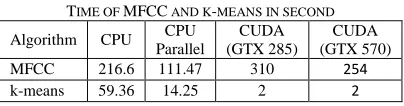
The results of calculations were presented while omitting the file read/write operations to concentrate on algorithm’s speedup. The results were performed on around data size of

350,000 feature vectors belonging to 92 female speakers. The Table II shows the actual times taken to perform MFCC and k-means algorithm in seconds.

TABLEII

TIME OF MFCC AND K-MEANS IN SECOND

Algorithm CPU CPU Parallel

CUDA (GTX 285)

CUDA (GTX 570) MFCC 216.6 111.47 310 254

k-means 59.36 14.25 2 2

It can be observed that the experimented MFCC algorithm has poor performance compared to traditional CPU algorithm. The reasons for this are the following:

- The only parallelized function within MFCC was discrete flourier transform algorithm. Although the complexity is reduced in theory, given the size of the problem for a single DFT run, it is not feasible to distribute the sub-problem into too many threads. For this experiment the size of outer loop was 240 and hence 240 threads were activated, but because of the low occupancy level the time needed to read/write into device global memory affected the performance.

- The other reason is low throughput of memory transfer between host and device. The DFT algorithm is called almost 350,000 times and each time it copies the window frames from host to device and copies the results of DFT back to host memory.

In k-means algorithm a considerable performance improvement can be seen when data-parallelism is compared to single threaded CPU. However the time taken on both GPU architectures is the same. One reason for this can be lack of use of shared memory to benefit from the architecture specific advantages. This may also indicate that current algorithm suffers from memory partition camping [16]. Global memory accesses go through partitions. Successive 256-byte regions of global memory are assigned to successive partitions. The problem of partition camping is when global memory accesses at an instant use a subset of partitions. This may hide the true potential of speedup scalability across cores. For optimal performance GPU accesses should be distributed evenly among partitions.

The results of EM algorithm are measured in parts to show the execution times more clearly. Table III shows the EM time in seconds.

TABLEIII

TIME OF EXPECTATION MAXIMIZATION IN SECONDS

Algorithm CPU CPU

Parallel GTX 285 GTX 570 SUM_P Per EM Iteration 56 17 3 2 Updating Mean,Var & Weight

Per EM Iteration 159 45.27 27 10 EM total per iteration 215 62.27 30 12

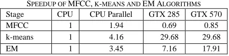
Again, faster calculations on more cores and further on many cores of GPUs can be seen. Table IV shows the speedup of all algorithms on different systems. The speedups are

1. Initialize mean, variance and weight values.

2. T = Number of feature vectors. (around 350K)

3. M = Order of mixtures (1024)

4. D = Number of dimensions in a feature vector (16)

5. Allocate memory on device and transfer the initialized

mean, variance and weight.

6. Transfer feature vectors to device memory.

8. Calculate Determinant of Sigma on 2 blocks of size M/2;

9. Calculate Sum p denominator on

T / 20 + 1 blocks of size 20;

11. Initialize SumMean and SumVariance on

1 block of size D;

12. Calculate SumMean and SumVariance on

T / 32 + 1 blocks of size 32;

13. Update Mean & Variance on 1 block of size D;

14. Update Weight on 1 block of size 1; }

15. Transfer mean, weight and variance from device to host

(7)

calculated using t1 / t2 where t1 is the single threaded CPU time and t2 is the target parallel model time. Additionally, Fig. 4 shows the graph corresponding to Table IV.

TABLEIV

SPEEDUP OF MFCC, K-MEANS AND EMALGORITHMS

Stage CPU CPU Parallel GTX 285 GTX 570 MFCC 1 1.94 0.69 0.85 k-means 1 4.16 29.68 29.68 EM 1 3.45 7.16 17.91

It is observed that the increase in the number of cores will decrease the calculation time. However, the technique of choosing the correct grid and block sizes should be taken into consideration. Too little threads in a block may race against the occupancy factor of the active blocks [10]. Too many threads in a block may prevent the use of shared memory since there is a limit of 16KB on GTX 285 and 48KB on GTX 570 models per block. In this study, a naïve GPU code that uses the global memory was provided. The number of threads used per CUDA block varies from 1 to 32. That is because current implementations performed better in low block dimension sizes. According to [12] in some cases such as [13] a better performance may be achieved in very low block sizes.

Fig. 4. Speedup scalability

VI. CONCLUSION

In this paper, a CUDA based implementation of DFT, k-means and EM algorithms were introduced. Also, the CPU parallelism of the mentioned algorithms for better comparison was presented. The results demonstrate the advantage of parallelization, specifically using GPUs to speed up calculation of k-means up to 30 times and EM up to 17.9 times of a single threaded CPU. In the future, the effects of using shared memory on the performance will be studied. Additionally, running the algorithms concurrently on more than one GPU will be presented to show how GPUs can benefit from cross device memory access [10]. Additionally, the advantage of concurrent kernels and multi streams will be experimented. Furthermore, a comparison between the performance hits of single-precision and double-precision

floating point calculations will be observed.

REFERENCES

[1] N. M. Laird, and D.B. Rubin A. P. Dempster, "Maximum Likelihood from Incomplete Data via EM Algorithm," Journal of the Royal Statistical Society, vol. 39, pp. 1-38, 1977.

[2] Green500. (2011, June) Green500. [Online]. http://www.green500.org/lists.php

[3] Intel. (2011, June) Previous Generation Intel® Core™ i7 Processor. [Online].

http://www.intel.com/products/processor/previousgenerationcorei7/inde x.htm

[4] N. Kumar, S. Satoor, and I. Buck, "Fast Parallel Expectation Maximization for Gaussian Mixture Models on GPUs Using CUDA," in

High Performance Computing and Communication, 11th IEEE International Conference on, 2009, pp. 103-109.

[5] R. W. Schafer and L. R. Tabiner, "Digital Repesentations of Speech Signals," IEEE Proceedings, vol. 63, pp. 662-667, April 1975. [6] Richard O. Duda, Peter E. Hart, and David G. Strok, Pattern

Classification, 2nd ed.: John Wiley and Sons, 2001.

[7] Wikipedia. (2011, June) Expectation-maximization algorithm. [Online]. http://en.wikipedia.org/wiki/Expectation_maximization_algorithm [8] D.A. Rose, R.C. Reynolds, "Robust text-independent speaker

identification using Gaussian mixture speaker models," Speech and Audio Processing, IEEE Transactions on, vol. 3, no. 1, p. 72, Jan 1995. [9] A. M. Kondoz, Digital Speech: Coding for Low Bit Rate

Communication Systems, 2nd ed.: Wiley, 2004.

[10] NVIDIA. (2011, March) NVIDIA CUDA Programming Guide - Version 4.0. [Online]. http://developer.nvidia.com/cuda-toolkit-40 [11] Wikipedia. (2011, June) CUDA. [Online].

http://en.wikipedia.org/wiki/CUDA

[12] V. Volkov. (2011, June) Better Performance at Lower Occupancy, GTC On-Demand: GTC 2010. [Online]. http://www.gputechconf.com/page/gtc-on-demand.html#session2238 [13] Anas Mohd Nazlee and Noohul Basheer Zain Ali Fawnizu Azmadi

Hussin, "Tranformation of CPU-based Applications To Leverage on Graphics Processors using CUDA," IJECS: International Journal of Electrical & Computer Sciences, vol. 10, no. 1, pp. 40-47, February 2010.

[14] "IEEE Standard for Floating-Point Arithmetic," IEEE Std 754-2008, pp. 1-58, August 2008.

[15] "Speech Codec Detector Based Speaker Verification System in a Multi-Coder Environment," doctoral dissertation, Computer Engineering Department, Eastern Mediterranean University, Famagusta, Mersin 10 Turkey, 2004. C. Ergün,.