Local Boosting of Decision Stumps for
Regression and Classification Problems
S. B. Kotsiantis
Educational Software Development Laboratory, Department of Mathematics, University of Patras, Greece Email: [email protected]
D. Kanellopoulos and P. E. Pintelas
Educational Software Development Laboratory, Department of Mathematics, University of Patras, Greece Email: [email protected], [email protected]
Abstract— Numerous data mining problems involve an investigation of associations between features in heterogeneous datasets, where different prediction models can be more suitable for different regions. We propose a technique of boosting localized weak learners; rather than having constant weights attached to each learner (as in standard boosting approaches), we allow weights to be functions over the input domain. In order to find out these functions, we recognize local regions having similar characteristics and then build local experts on each of these regions describing the association between the data characteristics and the target value. We performed a comparison with other well known combining methods on standard classification and regression benchmark datasets using decision stump as based learner, and the proposed technique produced the most accurate results.
Index Terms—classifier, machine learning, data mining, regressor
I. INTRODUCTION
Data is generated from an unknown distribution P on some domain X and labeled according to an unknown function g. A learning algorithm receives a sample S = {(x1, g(x1)), . . . , (xm, g(xm))} and attempts to return a function f close to g on the domain X. The target value is a discrete value in classification problems while it is a continuous value in regression problems. Many classification and regression problems involve an investigation of relationships between attributes in databases, where different prediction models can be more appropriate for different regions.
Instance-based learners classify an instance by comparing it to a database of pre-classified examples. The essential assumption is that similar instances will have similar target values. The corresponding components of an instance-based learner are the distance
function which determines how similar two instances are, and the prediction function which specifies how instance similarities yield a final prediction for the new instance [1].
Local learning [2] allows extending simple models, to the case of complex data for which the model’s assumptions would not necessarily hold globally, but can be thought as valid locally. A simple example is the assumption of linear separability, which in general is not satisfied globally in classification problems with rich data. Yet any classification algorithm able to find only a linear separation, can be used inside a local learning procedure, yielding an algorithm able to model complex non-linear class boundaries.
There has been much research work on ensemble learning for regression in the context of neural networks, however there has been less research carried out in terms of using homogeneous ensemble techniques to improve the performance of simple regression algorithms. Classification problems have dominated research on boosting to date. The application of boosting to regression problems, on the other hand, has received little investigation. In this paper we develop a boosting method for classification and regression problems that works locally. Usual boosting algorithms are well known to be sensitive to noise [5]. In the case of local boosting, the algorithm should handle reasonable noise, and be at least as good as boosting, if not better. For the experiments, decision stump was used as base learner. We performed a comparison with other well known combining methods on standard classification and regression benchmark datasets using decision stump as based learner, and the proposed technique produced the most accurate results.
In the next section, we discuss the localized experts, while current ensemble approaches and work are described in section 3. In Section 4 we describe the proposed method and investigate its advantages and limitations. In Section 5, we evaluate the proposed method on several UCI datasets by comparing it with standard combining techniques and other lazy methods. Finally, section 6 concludes the paper and suggests further directions in current research.
II. LOCALWEIGHTEDLEARNING
When all training instances are used when predicting the value of a new test case, the algorithm works as a global method, while when the nearest training examples are used, the algorithm works as a local method, since only data local to the area around the testing instance contribute to the prediction. Local methods have significant advantages when the probability measure defined on the space of symbolic objects is very complex, but can still be described by a collection of less complex local approximations.
When the size of the training set is small compared to the complexity of the learner, the learning machine usually overfits the noise in the training data. Thus effective control of complexity of a learner plays a key role in achieving good generalization. Several theoretical results and experimental results [19], [22] point out that a local learning algorithm provides a feasible solution to this problem.
In fact, local learning is not a new concept and it has appeared in the early years of pattern recognition. The obvious example is the k-nearest neighbor method: given a testing pattern, we estimate its target value from the closest pattern in the training set.
A list of objections to k-nearest neighbor algorithms includes the following: a) voting/averaging used to combine the values of the nearest k instances, b) uniform neighborhood shape (spherical) regardless of instance location and c) uniform weight given to all features, instances and neighbors
Our ultimate goal is not to improve the nearest neighbor algorithm, but to improve the accuracy by combining local learners. The authors of [7] proposed a theoretical model of a local learning algorithm and obtained bounds for the local risk minimization estimator for pattern recognition and regression problems using structural risk minimization principle.
In local learning, each local model is trained entirely independently of all other local models such that the total number of local models in the learning system does not straight influence how complex a function can be learned - complexity can only be controlled by the level of adaptability of each local model. This property avoids overfitting if a robust learning scheme exists for training the individual local model.
The authors of [9] extended the idea of constructing local simple base learners for different regions of input space, searching for appropriate architectures that should be locally used and for a criterion to select a proper unit for each region of input space. They proposed a hybrid MLP/RBF network by combining RBF and Perceptron units in the same hidden layer and using a forward selection to add units until an error goal is reached. Although the resulting Hybrid Perceptron/Radial Network is not in a strict sense an ensemble, the way by which the regions of the input space and the computational units are selected and tested could be in principle extended to ensembles of learning machines.
III. ENSEMBLESOFCLASSIFICATIONAND REGRESSIONMODELS
Empirical studies showed that ensembles are often much more accurate than the individual base learners that make them up [5], and recently different theoretical explanations have been proposed to justify the effectiveness of some commonly used ensemble methods [16]. Currently, there are two main approaches to model combination. The first is to produce a set of learned models by applying an algorithm repeatedly to different training sample data; the second applies various learning algorithms to the same sample data. The predictions of the models are then combined according to an averaging/voting scheme or a stacking algorithm [16].
In this work we propose a combining method that uses one learning algorithm for building an ensemble of regression models. For this reason this section presents the most well-known methods that generate sets of base learners using one base learning algorithm.
Starting with bagging [8], we will say that this method samples the training set, generates random independent bootstrap replicates, constructs a learner on each of these, and aggregates them by a simple majority vote or averaging procedure. Therefore, taking a bootstrap replicate one can sometimes avoid or get less misleading training objects in the bootstrap training set. Consequently, a learner constructed on such a training set may have a better performance.
Another method that uses different subset of training data with a single learning method is the boosting approach [13]. It assigns weights to the training instances, and these weight values are changed depending upon how well the associated training instance is learned by the learner; the weights for misclassified instances are increased. Thus, re-sampling occurs based on how well the training samples are classified by the previous model. Since the training set for one model depends on the previous model, boosting requires sequential runs and thus is not readily adapted to a parallel environment. After several cycles, the prediction is performed by taking a weighted vote of the predictions of each learner, with the weights being proportional to each learner’s accuracy on its training set.
AdaBoost is a practical version of the boosting approach for classification problems [13]. There are two ways that Adaboost can use these weights to construct a new training set to give to the base learning algorithm. In boosting by sampling, examples are drawn with replacement with probability proportional to their weights. The second method, boosting by weighting, can be used with base learning algorithms that can accept a weighted training set directly. With such algorithms, the entire training set (with associated weights) is given to the base-learning algorithm.
of its current master hypothesis on xi. The base learner then finds a function in a class minimizing the squared error on this constructed sample.
MultiBoosting [23] is another classification method of the same category that can be considered as wagging committees formed by AdaBoost. Wagging is a variant of bagging; bagging uses resampling to get the datasets for training and producing a weak hypothesis, whereas wagging uses reweighting for each training example, pursuing the effect of bagging in a different way.
In [20] another classification meta-learner (DECORATE, Diverse Ensemble Creation by Oppositional Relabeling of Artificial Training Examples) is presented that uses a learner to build a diverse committee. This is accomplished by adding different randomly constructed examples to the training set when building new committee members. These artificially constructed examples are given category labels that disagree with the current decision of the committee, thereby directly increasing diversity when a new classifier is trained on the augmented data and added to the committee.
IV. PROPOSEDALGORITHM
It is known that boosting is an effective technique for improving prediction accuracy in many real life datasets [5]. However, previous researches indicated that in heterogeneous databases, where several homogeneous regions exist, boosting does not enhance the prediction capabilities as well as for homogeneous databases [18]. In such cases our experiments indicate that it is more useful to have several local experts responsible for each region of the dataset.
The proposed algorithm builds a model for each point to be estimated, taking into account only a subset of the training points. This subset is chosen on the basis of the preferable distance metric between the testing point and the training point in the input space. For each testing point, a boosting ensemble of a weak learner is thus learned using only the training points lying close to the current testing point.
Generally, the proposed ensemble consists of the four steps (see Figure 1)
1) Determine a suitable distance metric.
2) Find the k nearest neighbors using the selected distance metric.
3) Apply boosting to the DS algorithm using as training instances the k instances
4) The answer of the boosting ensemble is the prediction for the testing instance.
Figure 1. Local Boosting ensemble
The proposed ensemble has some free parameters such as the distance metric. In our experiments, we used the most well known -Euclidean similarity function- as distance metric. For two data points, X = <x1, x2, x3, …, xn-1> and Y = <y1, y2, y3, …, y n-1>, the Euclidean similarity function is defined as .
The performance of ADABoost.M1 has been shown to exceed or meet that of various other boosting algorithms for classification [13], thus making it a good choice for this research. The performance of additive regression has been shown to exceed or meet that of various other boosting algorithms for regression [14], thus making it a good choice for this research. We used 10 iterations for the boosting process in order to reduce the time need for predicting the value of a new instance.
Decision stumps (DS) are one level decision trees [15]. We can find the best stump just as we would learn a node in a decision tree: we search over all possible features to split on, and for each one, we search over all possible thresholds induced by sorting the observed values. In classification problems, each node in a decision stump represents a feature in an instance to be classified, and each branch represents a value that the node can take. Instances are classified starting at the root node and sorting them based on their feature values. In regression problems, DS (or regression stumps) do regression based on mean-squared error where each node in a decision stump represents a feature in an instance to be predicted, and each branch represents a value that the node can take. At worst a decision stump will reproduce the most common sense baseline, and may do better if the selected feature is particularly informative.
The proposed algorithm also requires choosing the value of K. There are several ways to do this. A first, simple solution is to fix K a priori before the beginning of the learning process. However, the best K for a specific dataset is obviously not the best one for another dataset. A second, more time-consuming solution is therefore to determine this best K automatically through the minimization of a cost criterion. One way to do that is to evaluate the estimation error on a test set and thus keep as K the value for which the error is the least. In the current implementation we decided to use a fixed value for K (=50): a) in order to keep the training time low and b) about this size of instances is appropriate for a simple algorithm, to build a precise model according to [12], [19].
Our method shares the properties of other memory-based methods such as no need for training and more computational cost for the prediction. Besides, our method has some desirable properties, such as better accuracy and confidence interval.
V. EXPERIMENTS
We perform comparisons with other well known combining methods on classification and regression problems.
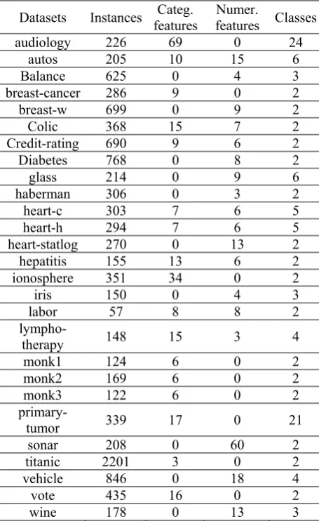
TABLE I. THE USED CLASSIFICATION DATASETS
Datasets Instances features Categ. features Numer. Classes
audiology 226 69 0 24
autos 205 10 15 6 Balance 625 0 4 3
breast-cancer 286 9 0 2
breast-w 699 0 9 2
Colic 368 15 7 2
Credit-rating 690 9 6 2
Diabetes 768 0 8 2
glass 214 0 9 6
haberman 306 0 3 2
heart-c 303 7 6 5 heart-h 294 7 6 5
heart-statlog 270 0 13 2
hepatitis 155 13 6 2
ionosphere 351 34 0 2
iris 150 0 4 3
labor 57 8 8 2
lympho-therapy 148 15 3 4
monk1 124 6 0 2 monk2 169 6 0 2 monk3 122 6 0 2
primary-tumor 339 17 0 21
sonar 208 0 60 2 titanic 2201 3 0 2 vehicle 846 0 18 4
vote 435 16 0 2
wine 178 0 13 3
In order to calculate the classifiers’ accuracy, the whole training set was divided into ten mutually exclusive and equal-sized subsets and for each subset the classifier was trained on the union of all of the other subsets. Then, cross validation was run 10 times for each algorithm and the average value of the 10-cross validations was calculated. It must be mentioned that we used the free available source code for most of the algorithms by [25] for our experiments.
We compare the proposed ensemble methodology with:
• K-nearest neighbors using k=3 (most common used number of neighbors), as well as k=50 because the proposed algorithm uses 50 neighbors. In addition, we tested Kstar: another instance-based learner which uses entropy as distance measure [11].
• Local weighted DS using 50 instances
• Bagging DS, Boosting DS and MultiBoost DS (using 25 sub-classifiers)
• DECORATE DS
In following Tables, we represent as “v” that the specific algorithm performed statistically better than the proposed ensemble according to t-test with p<0.05. Throughout, we speak of two results for a dataset as being "significant different" if the difference is statistical
resampled t-test [21], with each pair of data points consisting of the estimates obtained in one of the 100 folds for the two learning methods being compared. On the other hand, “*” indicates that the proposed ensemble performed statistically better than the specific algorithm according to t-test with p<0.05. In all the other cases, there is no significant statistical difference between the results (Draws). In the last row of the table one can also see the aggregated results in the form (α/b/c). In this notation “α” means that the proposed ensemble is significantly less accurate than the compared algorithm in
α out of 27 datasets, “c” means that the proposed algorithm is significantly more accurate than the compared algorithm in c out of 27 datasets, while in the remaining cases (b), there is no significant statistical difference.
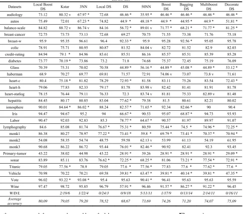
In the last raw of the Table II one can see the aggregated results. The presented ensemble is significantly more accurate than single DS in 18 out of the 27 datasets, while it has significantly higher error rate in none dataset. What is more, the proposed ensemble is significantly more accurate than 3NN and 50NN in 4 and 11 out of the 27 datasets, respectively, whilst it has significantly higher error rate in one and 5 datasets. Likewise, the proposed ensemble is significantly more accurate than local weighted DS and Kstar in 3 and 6 out of the 27 datasets, whilst it has significantly higher error rate in none and two datasets, respectively. In addition, local boosting is significantly more accurate than Bagging DS in 14 out of the 27 datasets, whilst it has significantly higher error rate in none dataset. Furthermore, Multiboost DS and Decorate DS have significantly lower error rates in 2 and none out of the 27 datasets than the proposed ensemble, respectively whereas they are significantly less accurate in 11 datasets. Adaboost DS has significantly lower error rates in 1 out of the 27 datasets than local boosting, whereas it is significantly less accurate in 9 datasets.
To sum up, the performance of the presented ensemble is more accurate than the other well-known ensembles that use only the DS algorithm. The proposed ensemble can achieve an increase in classification accuracy about 17% compared to simple DS. The average relative accuracy improvement of the proposed methodology is from 1.5% to 12.5% in relation to the remaining methods. This indicates that it is possible to obtain a feasible solution to problems of pattern classification in the real world by local learning because approximating global target function is hard given that usually not enough training samples are available.
TABLE II. COMPARING LOCAL BOOSTING DS WITH INSTANCE BASED CLASSIFIERS AND OTHER ENSEMBLES THAT USE DS AS BASE LEARNER
Datasets Local Boost DS Kstar 3NN Local DS DS 50NN Boost DS Bagging DS Multiboost DS Decorate DS
audiology 73.12 80.32 v 67.97 * 72.68 46.46 * 35.95 * 46.46 * 46.46 * 46.46 * 46.46 * autos 75.49 72.01 67.23 * 74.82 44.9 * 48.18 * 44.9 * 44.95 * 44.9 * 51.81 * balance-scale 84.82 88.72 v 86.74 v 84.16 56.72 * 89.01 v 71.77 * 68.21 * 71.77 * 81.25 * breast-cancer 72.75 73.73 73.13 72.68 69.27 70.75 71.55 73.38 71.76 75.18
breast-w 95.9 95.35 96.61 96.4 92.33 * 95.9 95.28 92.56 * 95.05 95.78
colic 78.91 75.71 80.95 80.87 81.52 84.04 v 82.72 81.52 82.9 82.03 credit-rating 84.94 79.1 * 84.96 83.61 85.51 86.16 85.57 85.51 85.39 85.28
diabetes 73.77 70.19 * 73.86 73.2 71.8 74.68 75.37 72.45 75.19 76.09 Glass 70.39 75.31 70.02 70.58 44.89 * 56.16 * 44.89 * 45.08 * 44.89 * 53.12 * haberman 68.9 70.27 69.77 69.81 71.57 72.91 74.06 v 73.07 73.8 v 71.61
heart-c 80.4 75.18 * 81.82 78.29 72.93 * 81.58 83.11 75.26 83.54 72.43 * heart-h 79.06 77.83 82.33 79.17 81.78 83.98 v 82.42 81.41 81.91 81.78 heart-statlog 78.15 76.44 79.11 76.33 72.3 83.74 v 81.81 75.33 82.89 v 81.48
hepatitis 84.45 80.17 80.85 83.04 77.62 * 79.38 81.5 80.61 82.21 80.02 ionosphere 90.01 84.64 * 86.02 * 88.24 82.57 * 71.65 * 92.34 82.66 * 90 90.4
Iris 94.47 94.67 95.2 94 66.67 * 90.53 95.07 68.87 * 94.73 93.93 Labor 90.47 92.03 92.83 85.3 78.77 * 64.67 * 90.57 81.97 89.97 91.07 lymphography 84.6 85.08 81.74 76.67 * 75.31 * 80.59 75.44 * 74.5 * 74.96 * 72.25 *
monk1 86.38 80.27 78.97 77.22 * 73.41 * 59.8 * 69.79 * 73.41 * 70.37 * 70.94 * monk2 54.08 58.35 54.74 48.75 59.58 62.13 v 53.99 61.13 54.19 61.95 monk3 90.68 86.22 86.72 93.44 76.01 * 82.46 * 90.92 82.41 92.3 93.45
Primary-tumor 43.22 38.02 44.98 43.22 28.91 * 39.26 28.91 * 28.91 * 28.91 * 29.09 * sonar 83.89 85.11 83.76 76.62 * 72.25 * 68.25 * 81.06 73.21 * 77.54 * 72.91 * Titanic 79.05 77.56 * 78.9 79.05 77.6 * 77.56 * 77.83 77.6 * 77.62 * 77.6 * Vehicle 70.98 70.22 70.21 69.58 39.81 * 63.47 * 39.81 * 40.14 * 39.81 * 47.35 * Vote 96.02 93.22 * 93.08 * 95.4 95.63 90.41 * 96.41 95.63 95.63 95.59 Wine 97.47 98.72 95.85 96.79 57.91 * 96.46 91.57 * 86.27 * 91.22 * 96.45
W/D/L 2/19/6 1/22/4 0/24/3 0/9/18 5/11/11 1/17/9 0/13/14 2/14/11 0/16/11
Average
accuracy 80,09 79,05 79,20 78,52 68,67 73,69 74,26 71,20 74,07 75,09
Firstly, we compared the proposed ensemble methodology with other methods that are based on the same learning algorithm - DS:
• Simple DS algorithm
• Local DS using 50 local instances. This method differs from the proposed technique since it has no boosting process.
• Bagging DS and Additive regression DS (using 10 sub-models). Both these methods work globally whereas the proposed method works locally.
The most well known measure for the degree of fit for a regression model to a dataset is the correlation coefficient. If the actual target values are a1,a2, … an, and the predicted target values are: p1,p2, … pnthen the correlation coefficient
is given by the formula:
A P PA
S
S
S
R
=
,where1 ) )( (
− − −
=
∑
n a a p p
S i
i i
PA ,
1 )
( 2
− −
=
∑
n p p
S i
i
P , 1
)
( 2
− − =
∑
n a a
S i
i
A ,
p
: the average value of pi anda
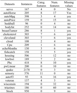
: the average value of αi.Similarly, in order to calculate the models’ correlation coefficient for our experiments, cross validation was run 10 times for each algorithm and the average value of the 10-cross validations was calculated. It must be mentioned that we used the free available source code for most of the algorithms by [25] for our experiments, too.
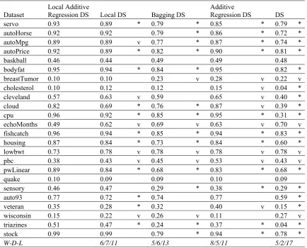
significantly higher error rate in 5 datasets. Furthermore, global additive regression DS have significantly lower error rates in 8 datasets than the proposed ensemble, whereas it is significantly less accurate in 11 datasets.
TABLE III. THE USED REGRESSION DATASETS
Datasets Instances features Categ. features Num. Missing values servo 167 4 0 No
autoHorse 205 8 17 Yes
autoMpg 398 3 4 yes
autoPrice 159 0 15 no
baskball 96 0 4 no
bodyfat 252 0 14 no
breastTumor 286 8 1 yes
cholesterol 303 7 6 yes
cleveland 303 7 6 yes cloud 108 2 4 no
Cpu 209 1 6 no
echoMonths 130 3 6 yes
fishcatch 158 2 5 yes housing 506 1 12 no lowbwt 189 7 2 no
Pbc 418 8 10 yes
pwLinear 200 0 10 no quake 2178 0 3 no sensory 576 11 0 no
auto93 93 6 16 yes
veteran 137 4 3 no wisconsin 194 0 32 no
triazines 186 0 60 no Stock 950 0 9 no
To sum up, the performance of the presented ensemble is better than the other well-known ensembles that use only the DS algorithm. This indicates that it is possible to obtain a feasible solution to regression problems in the real world by local additive regression because approximating a global target function is hard given that usually not enough training samples are available.
Several other models have been proposed for modeling and approximating the values of a continuous objective attribute by using the values of conditional attributes, such as local learners, regression trees, and neural networks.
Subsequently, we compared the proposed ensemble methodology with other well known regression algorithms: • K-nearest neighbors using k=50 because the proposed
algorithm uses 50 neighbors. In addition, we tested Kstar: another instance-based learner which uses entropy as distance measure [11].
• The most well known algorithm for training artificial neural networks – Back Propagation (BP) with one hidden layer and five neurons in this layer [25].
• A well known regression tree algorithm - RepTree [25] • A well known regression algorithm - Decision Table
[15]
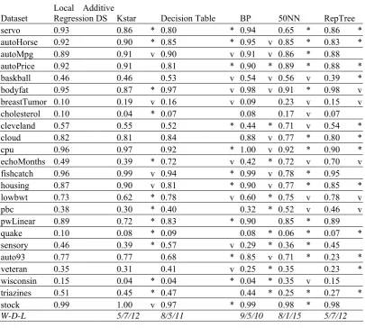
In the last raw of Table V one can see the aggregated results. The proposed ensemble is significantly more accurate than simple Kstar in 12 out of the 24 datasets, whilst it has significantly higher error rate in 5 datasets. In addition, the presented ensemble is significantly more accurate than 50NN in 15 out of the 24 datasets, while it has significantly higher error rate in 8 datasets. What is more, the proposed ensemble is significantly more accurate than Decision Table in 11 out of the 24 datasets, whilst it has significantly higher error rate in 8 datasets. Furthermore, the BP algorithm has significantly lower error rates in 9 datasets than the proposed ensemble, whereas it is significantly less accurate in 10 datasets. Finally, the RepTree algorithm has significantly lower error rates in 12 datasets than the proposed ensemble, whereas it is significantly less accurate in 7 datasets. To sum up, the performance of the presented ensemble is more accurate than the other well-known regression methods.
VI. CONCLUSION
Local algorithms defer processing of the dataset until they receive request for information (e.g. classification or prediction of target value). A database of observed input-output data is always kept and the estimate for a new operating point is derived from an interpolation based on a neighborhood of the query point. Local techniques are an old idea in time series prediction [3].
Lazy learners are particularly useful for prediction on data streams. In data streams, new data keep arriving, so building a new learner each time can be very expensive. In addition, the multidimensional data is sometimes feature-space heterogeneous so that different features have different importance in different sub-areas of the whole space.
Local learning can reduce the complexity of component learners and improve the generalization performance although the global complexity of the system can not be guaranteed to be low. In this paper we propose local boosting and our experiment for some real datasets shows that the proposed combining method outperforms other well known combining classification and regression methods as well as any individual learner.
Usual boosting algorithms are well known to be sensitive to noise [5]. In the case of local boosting, the algorithm should handle reasonable noise, and be at least as good as boosting, if not better. Due to the encouraging results obtained from our experiments, we can expect that the proposed combining method can be successfully applied to the classification and regression task in the real world case with more accurate results than the traditional data mining approaches.
TABLE IV. COMPARING LOCAL ADDITIVE REGRESSION DS WITH OTHER TECHNIQUES THAT USE DS AS BASE LEARNER
Dataset
Local Additive
Regression DS Local DS Bagging DS
Additive
Regression DS DS
servo 0.93 0.89 * 0.79 * 0.85 * 0.79 *
autoHorse 0.92 0.92 0.79 * 0.86 * 0.72 *
autoMpg 0.89 0.89 v 0.77 * 0.87 * 0.74 *
autoPrice 0.92 0.89 * 0.82 * 0.90 * 0.81 *
baskball 0.46 0.44 0.49 0.49 0.48
bodyfat 0.95 0.94 * 0.84 * 0.95 0.82 *
breastTumor 0.10 0.10 0.23 v 0.28 v 0.22 v
cholesterol 0.10 0.12 0.12 0.15 v 0.04 *
cleveland 0.57 0.63 v 0.59 0.65 v 0.40 *
cloud 0.82 0.69 * 0.76 * 0.87 v 0.39 *
cpu 0.96 0.92 * 0.85 * 0.95 * 0.31 *
echoMonths 0.49 0.62 v 0.69 v 0.63 v 0.70 v
fishcatch 0.96 0.94 * 0.85 * 0.94 * 0.83 *
housing 0.87 0.84 * 0.73 * 0.84 * 0.60 *
lowbwt 0.73 0.78 v 0.78 v 0.78 v 0.78 v
pbc 0.38 0.43 v 0.45 v 0.53 v 0.43 v
pwLinear 0.89 0.84 * 0.68 * 0.83 * 0.68 *
quake 0.10 0.09 0.09 0.10 0.09
sensory 0.46 0.47 0.29 * 0.38 * 0.29 *
auto93 0.77 0.72 * 0.74 0.77 0.59 *
veteran 0.35 0.28 * 0.32 0.40 v 0.15 *
wisconsin 0.15 0.22 v 0.26 v 0.11 0.27 v
triazines 0.51 0.47 * 0.24 * 0.37 * 0.04 *
stock 0.99 0.99 0.79 * 0.94 * 0.78 *
W-D-L 6/7/11 5/6/13 8/5/11 5/2/17
By removing a set of instances from a database the response time for the predictions will decrease, as fewer instances are examined when a query instance is presented. This objective is primary when we are working with large databases and have limited storage.
In a following work we will focus on the problem of reducing the size of the stored set of instances while trying to maintain or even improve generalization accuracy by avoiding noise and overfitting. In [6] and [24] can be found numerous instance selection methods that can be combined with local boosting technique.
REFERENCES
[1] D. Aha, Lazy Learning. Dordrecht: Kluwer Academic
Publishers, 1997.
[2] C. G. Atkeson, A. W. Moore, and S. Schaal, Locally weighted learning for control. Artificial Intelligence Review, 11:75–113,
1997.
[3] C.G. Atkeson, A.W. Moore & S. Schaal, Locally weighted learning. Artificial Intelligence Review, 11(1-5), 11-73, 1997.
[4] C. Blake & C. Merz, UCI Repository of machine learning databases. Irvine, CA: University of California, Department of Information and Computer Science. http://www.ics.uci.edu/~mlearn/MLRepository.html
[5] E. Bauer and R.. Kohavi. An empirical comparison of voting classification algorithms: Bagging, boosting and variants. Machine Learning, 36(1/2):525–536, 1999.
[6] H. Brighton, C. Mellish, Advances in Instance Selection for Instance-Based Learning Algorithms, Data Mining and Knowledge Discovery, 6, 153–172, 2002.
[7] L. Bottou and V. Vapnik, Local learning algorithm,
Neural Computation, vol. 4, no. 6, pp. 888-901, 1992.
[8] L. Breiman, Bagging Predictors. Machine Learning, 24(3),
123-140. Kluwer Academic Publishers, 1996.
[9] S. Cohen and N. Intrator. Automatic Model Selection in a Hybrid Perceptron/ Radial Network. In Multiple Classifier Systems. 2nd Inter. Workshop, MCS 2001, pages 349–358. [10]Duffy, N. Helmbold, D., Boosting Methods for Regression,
Machine Learning, 47, (2002) 153–200.
[11]C. John and L. Trigg, K*: An Instance- based Learner Using an Entropic Distance Measure", Proc. of the 12th International Conference on ML, pp. 108-114, 1995.
[12]E. Frank, M. Hall and B. Pfahringer, Locally weighted naive Bayes. Proc. of the 19th Conference on Uncertainty in Artificial Intelligence. Mexico, 2003.
[13]Y. Freund and R. Schapire, Experiments with a New Boosting Algorithm, Proc. ICML’96, p. 148-156, 1996
TABLE V. COMPARING LOCAL ADDITIVE REGRESSION DS WITH OTHER LEARNERS
Dataset Local Additive Regression DS Kstar Decision Table BP 50NN RepTree
servo 0.93 0.86 * 0.80 * 0.94 0.65 * 0.86 *
autoHorse 0.92 0.90 * 0.85 * 0.95 v 0.85 * 0.83 *
autoMpg 0.89 0.91 v 0.90 v 0.91 v 0.86 * 0.88
autoPrice 0.92 0.91 0.81 * 0.90 * 0.89 * 0.88 *
baskball 0.46 0.46 0.53 v 0.54 v 0.56 v 0.39 *
bodyfat 0.95 0.87 * 0.97 v 0.98 v 0.91 * 0.98 v
breastTumor 0.10 0.19 v 0.16 v 0.09 0.23 v 0.15 v
cholesterol 0.10 0.04 * 0.07 0.08 0.17 v 0.07
cleveland 0.57 0.55 0.52 * 0.44 * 0.71 v 0.54 *
cloud 0.82 0.81 0.84 0.88 v 0.77 * 0.80 *
cpu 0.96 0.97 0.92 * 1.00 v 0.92 * 0.90 *
echoMonths 0.49 0.39 * 0.72 v 0.42 * 0.72 v 0.70 v
fishcatch 0.96 0.99 v 0.94 * 0.99 v 0.78 * 0.95
housing 0.87 0.90 v 0.81 * 0.90 v 0.77 * 0.85 *
lowbwt 0.73 0.62 * 0.78 v 0.60 * 0.75 v 0.78 v
pbc 0.38 0.30 * 0.40 0.32 * 0.52 v 0.46 v
pwLinear 0.89 0.72 * 0.83 * 0.90 0.85 * 0.89
quake 0.10 0.08 * 0.09 0.08 * 0.06 * 0.07 *
sensory 0.46 0.39 * 0.57 v 0.29 * 0.36 * 0.45
auto93 0.77 0.77 0.68 * 0.85 v 0.71 * 0.23 *
veteran 0.35 0.31 0.41 v 0.25 * 0.35 0.23 *
wisconsin 0.15 0.04 * 0.04 * 0.04 * 0.35 v 0.15
triazines 0.51 0.45 * 0.47 0.44 * 0.25 * 0.27 *
stock 0.99 1.00 v 0.97 * 0.99 0.98 * 0.98
W-D-L 5/7/12 8/5/11 9/5/10 8/1/15 5/7/12
[15]W. Iba, & P. Langley, Induction of one-level decision trees. Proc. of the Ninth Inter. Machine Learning Conference (1992). Scotland: Morgan Kaufmann.
[16]E.M. Kleinberg. A Mathematically Rigorous Foundation for Supervised Learning, volume 1857 of Lecture Notes in Computer Science, pages 67–76. Springer-Verlag, 2000. [17]Kohavi R., The Power of Decision Tables. In Proc
European Conference on ML (1995) 174 - 189.
[18]T. Lazarevic, Z. Obradovic, Adaptive Boosting for Spatial Functions with Unstable Driving Attributes, In Proc. of Pacific-Asia Conf. on Knowledge Discovery and Data Mining, 2000, pp. 329-340.
[19]Loader, C., Local Regression and Likelihood. Springer, New York, (1999).
[20]P. Melville and R. Mooney, Constructing Diverse Classifier Ensembles using Artificial Training Examples,
Proc. of the IJCAI-2003, pp.505-510, Mexico, 2003 [21]Nadeau, C., Bengio, Y., Inference for the Generalization
Error. Machine Learning, 52 (2003) 239-281.
[22]V.N. Vapnik, Statistical Learning Theory, Wiley, New
York, 1998.
[23]G. I. Webb, MultiBoosting: A Technique for Combining Boosting and Wagging, Machine Learning, 40, 159–196, Kluwer Academic Publishers, 2000.
[24]D. Wilson, and T. Martinez, Reduction Techniques for Instance-Based Learning Algorithms, Machine Learning,
38, 257–286, 2000.
[25] I. Witten, and E. Frank, Data Mining: Practical Machine Learning Tools and Techniques with Java Implementations. Morgan Kaufmann, San Mateo, CA, 2000.
S. B. Kotsiantis received a diploma in mathematics, a Master and a Ph.D. degree in computer science from the University of Patras, Greece. His research interests are in the field of data mining and machine learning. He has more than 50 publications to his credit in international journals and conferences.
D. Kanellopoulos received a diploma in electrical engineering and a Ph.D. degree in electrical and computer engineering from the University of Patras, Greece. He has more than 40 publications to his credit in international journals and conferences.