Iles

(1)

Forestry & Natural-Resource Sciences Last Correction: Aug. 28, 2009

“NEAREST-TREE” ESTIMATIONS

A discussion of their geometry

Kim Iles

Kim Iles & Associates Ltd., 412 Valley Place, Nanaimo, BC, Canada. Ph.&FAX: 250.753.8095

Abstract.The use of “nearest-neighbor” sampling has a long history. It involves measuring the distance

from a random point in an area to the nearest object. That history involves never quite solving the problem, many examinations of special cases that never occur, adjustments that were ad-hoc, and a great deal of uninformative algebra. In forestry we have attempted to use the “nearest-tree” method for estimating numbers of trees on a landscape but the method is general, and can be used for any objects being sampled.

I believe that the literature has never shown the logic and geometry in a form that is useful to both under-stand and solve the problem. This paper discusses the method from the geometric point of view, making no assumptions about tree distribution, and shows why extending the processes to the “nth_{closest tree” much} reduces the bias and variability, as well as specifying what is needed to solve the problem in an unbiased way.

Keywords:Unbiased methods, total-balancing, data adjustment, forest inventory, sampling methods

1 Background

For more than half a century, the idea of measuring distance from a random point to the nearest object has been developed. It has often been reviewed in the sam-pling literature, for instance in books by Pielou (1977), and Bonham (1989). Most of the history of the sub-ject seems to have been developed by ecologists or the mathematicians to whom they brought the problem.

My own interpretation of the method is that it devel-oped roughly as follows:

1) We can see that the average distance to objects, trees for instance, clearly decreases when more objects are added to a ﬁxed tract area – especially if the trees are not extremely clustered. Therefore, distances between random points and objects could be used to estimate the density (meaning objects per unit of land area – tree stems in this case).

2) As with many sampling systems, they looked at estimators based on a random distribution, even though this was clearly wrong. Generally, the area around each tree was computed using the distance to the nearest tree (r_i) by an equation known to be unbiased with a random distribution, then averaged to give area A_t. This area around the tree was then used to compute the number of trees in an area as follows:

N =

Tract area

At

This was highly satisfying for random distributions, although the mathematical proof of such a thing was not easy to follow or explain. Having the equation was enough.

3) A feeling of guilt developed in the ecological circles, since everyone knew that trees and other objects were not randomly distributed. No theoretical approach sug-gested itself, so a period of simulation followed and ex-amined quite a variety of estimations using the distance (r_i), such as detailed in Engeman (1994). As in all simu-lations, it was never “done in our own backyard” so any correction constants could not be trusted - no matter how interesting they might be.

Even with no bias, the method will typically give an answer that is too low. This is because of a high variabil-ity when some distances to the tree are very short and therefore give very large individual estimates of N. Al-though these few very large estimates make the system unbiased, they happen rarely enough that the median answer is typically too low. In this case it is arguably wise to use a biased estimate, which gives a smaller ac-tual error in most cases, and just live with the bias.

4) The problem was extended, in hopes that the vari-ability and any perceived bias would go away. Samplers looked at the 2nd_{-closest tree, the 3}rd_{, and generally the} “nth_{closest tree” hoping that the bias would} asymptoti-cally go away, and indeed that seemed to be the case.

5) At several times people realized that this was really

Copyright c2009 Publisher of the International Journal ofMathematical and Computational Forestry & Natural-Resource Sciences

(2)

a problem of deducing the area of the average Voronoi polygon around individual trees. Once you had that area, of course, that puts you into the well known realm of Horvitz-Thompson estimators and simpliﬁes every-thing. A Voronoi polygon is the area around a tree where it is the “closest” tree to any point in the polygon. In fact, the situation could be examined with any shape of polygon around trees, provided that the polygons tessel-lated the area and you could tell which polygon you fell into with a sample point. Voronoi polygons are simply a very convenient situation to consider.

I have never been able to find a simple procedure for calculating the Voronoi polygon area around a single tree while in the field. Solving the problem for thousands of trees with XY coordinates is easily done and quite efficient by computer algorithms, and you would think that perhaps a simple Excel program must be available to do this in the field using angles and distances to trees. I have not been able to find such a program.

I would suggest that perhaps this is one of those times when we could look at the geometry of the situation and perhaps gain some insight. Before samplers found out that calculus was so impressive to journal editors, they would reason out the geometry of various situa-tions and sometimes came up with some inspired results. Consider Walter Bitterlich’s development in the 1940’s of Angle-Count Sampling (typically called Variable Plot Sampling) as one example (Bitterlich, 1984). He devel-oped this as a geometry exercise, and it changed forest sampling worldwide. Perhaps this is another example that might beneﬁt from such an approach. Geometric proofs are, after all, a valid type of proof. They are every bit as mathematical as an algebraic or calculus approach, and can be much more illuminating.

2 The Geometry

Consider, ﬁrst, the geometry of selecting a tree lin-early “closest” to a random point. Clearly this is a question of falling within a Voronoi polygon in which that tree is “nearest”. Where other deﬁnitions of “clos-est” are considered, the geometry remains very similar and the solutions here are basically unchanged.

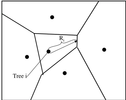
The average area of such polygons provides the key to estimating the number of trees per hectare. A ran-dom point in the area is always located in one and only one of these polygons, and falls within those polygons with probability proportional to their area. Figure 1 illustrates this situation.

3 The Problem

The question is: how can we estimate the polygon area by only using a linear distance? If we could detect the distance from the tree to the edge of this polygon,

Tree i

R_i

Figure 1: The “nearest-tree” Voronoi polygon, which is sampled, proportional to its size, by a random point.

a solution becomes fairly simple, and the variability of the estimator is much reduced. Consider the distance R_i, which is from the tree to the edge of the polygon. The edge is recognized because it is the point where one or more other trees are the same distance from tree i. A shorter distance r_i has traditionally been used as the distance from a random point to the tree. The larger distance R_i is the distance from a tree (or more gener-ally any ﬁxed point) to the edge of the polygon. This distance has some very fortunate characteristics.

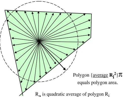
One of the examples in some calculus courses is to es-tablish that the quadratic average (R_a) of the distances R_i chosen with equal probability from any ﬁxed point (for instance the tree in the polygon) is equal to a circle having radius R_a with exactly the same area as that ir-regular polygon. This was discussed by Matern (1956), and more recently by Gregoire and Valentine (1995). The polygon does not need to have straight edges for this; but it does in our case, because the edges are formed from bisectors of adjacent trees. For nearest-tree situa-tions it is a very simple polygon with a reference point (the tree) which is easy to identify.

This also leads to the estimate:

R2

a×π

= polygon area

.

If we simply use R2

i ×π

in each case, and then av-erage the areas of these circles, we get an unbiased esti-mate ofR2

a×π

(3)

Polygon {average Ri2}

π

equals polygon area

.

R

_a

_{is quadratic average of polygon Ri}

Figure 2: A circle having a radius (R_a) equivalent to the

quadratic average of all possible distances

R2_i n , has an area equal to the area of that irregular polygon.

If the ray outward from the tree was not randomly chosen (such as when it was chosen by going through a random point) we would have to weight the individ-ual distances to compute the same expected value. Here again, we have only to refer to previous work. Walter Bitterlich taught foresters how to select circles propor-tional to their area and how to use the results. This simple geometry problem was solved by using an angle gauge to choose trees at a random point. A random point chooses the larger circles (radii) by the square of the radius involved.

If we wanted to have the arithmetic average of the radii as if the radii were chosen equally, the ﬁrst sug-gestion for this seems to have come from Hirata (1956). We simply take the harmonic mean of the squared radii, because the weighting of their selection was made with probability proportional to the squared distance. It is easy to imagine the weight being proportional to a small wedge extending from the tree outwards, so the proba-bility of a point falling into this area is proportional to the square of the distance:

Ra=

1 ⎛ ⎝ R12_i

n ⎞ ⎠

.

This is the unbiased estimate of the arithmetic mean of equally chosen radii, even though the radii used in this computation were chosen proportional to their squared length by going from the tree through a randomly chosen

point in the polygon.

How could we do this in the ﬁeld? Our problem is simply to sample for the average circle area (R2_a×π) using distances from the tree to the polygon edge. One way to do this is:

1) Select a random point and go to the nearest tree.

2) From the tree, select a random angle, and go in that direction until the edge of the polygon is en-countered. This is the ﬁrst point where another tree would be equally far away (R_i).

This “random direction” step can be skipped if you use the harmonic mean just described, in which case the distance R_iis from the tree through the sample point to the edge of the polygon. This simpliﬁes ﬁeld work.

3) Measure R_i, as an estimate of a circle radius equal to the polygon area. The average of these squared radii (weighted harmonically, if necessary) is R2_a. (R2_a×π) then estimates the average polygon area around individual trees.

4) From this, the number of trees/ha can be calcu-lated.

Other estimates of volumes, values and other charac-teristics are similarly best imagined geometrically, but will be more fully described in future papers. To those who are familiar with Variable Plot sampling, these are easily imagined as Volume to Basal Area Ratios (VBARs). When averaged, these can simply be mul-tiplied by stand area in order to produce totals for the tract.

It is relatively easy to do such calculations. The main deviation from previous work comes from viewing the problem as a sample of various size circles, rather than using any assumption at all about tree distribu-tion. Note that there is absolutely no restriction at all on the distribution of trees.

At this point, we have the same form of equation as has always existed for point to plant areas and numbers per hectare. The only diﬀerence is that the circle area derived from point to the plant distances (r_i) was dou-bled. This was used because when we choose a random point in a circle, the average area of (r2

i×π) is1/2of the

area (R2

i ×π).

(4)

This problem is also best viewed as a geometry prob-lem. Although some have apparently viewed this dis-tance to the nthtree as a kind of “plot radius” (Lynch, 2003), I believe that this does not provide insight into the actual geometry. Lately, several authors, for instance Magnussen (2008) and Kleinn (2006) deduced that this involved “order-k” Voronoi polygons (Okabe, et al, 1999, chapter 3, page 152) around trees, but admitted that calculating these in the ﬁeld was even more impractical. Indeed, measuring the polygon is too awkward to con-template, but sampling for it is not. Using many trees in a larger polygon, rather than just one nth_{-nearest tree} certainly complicates imagining the geometry.

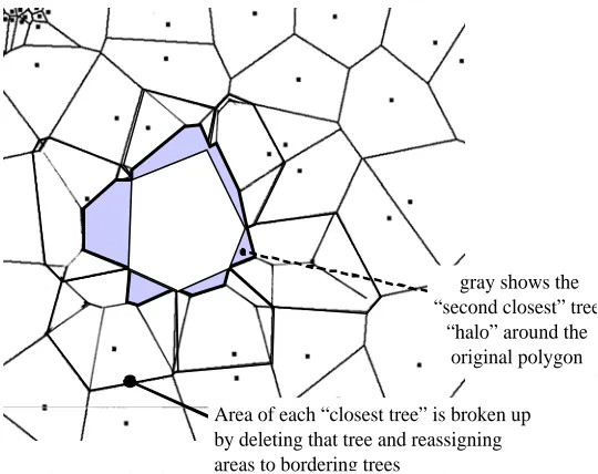
If you consider the Voronoi polygons around the near-est tree, and ask what is the polygon where this tree is the “2nd_{-nearest-tree”, the geometry begins to clear} up. In this illustration, I have taken the polygons for trees bordering an example tree and calculated the parts of these where the example tree is the 2nd_{-nearest-tree.} This can be done by hand, and I am sure that it could be done quickly and more accurately by a GIS sys-tem, which would be especially necessary for larger “nth -nearest” situations. The analysis depends upon individ-ually eliminating trees, then dividing that tree’s poly-gon among other trees. This process adds what I will call “slivers” along the edge each of the original Voronoi polygon. It is within these slivers that the tree is the 2nd-nearest-tree. You do not need to know this area or the boundaries, because you know when you fall into that polygon (because that example tree is the second closest), but visualizing the geometry reveals a lot about why it works well.

The graph from this process produces a “halo” (Fig. 3) of slivers which surrounds each tree. Here they are illus-trated around just one of the trees.

The consequence of this is that the starting point for the distance to the “n-th nearest-tree” must lie within these slivers. The outer border of the halo forms a new polygon consisting of the inner original polygon plus the added slivers. On the average, these larger polygons are exactly twice the size of the inner polygons describing the nearest trees. The smaller slivers add up to exactly the tract area, and are all allocated to one and only one tree. The interior parts of the original “nearest-tree” polygon would be divided into slivers which would select some other tree as the 2nd-closest. Therefore, the original polygons plus the sliver areas that border them amount to twice the area of the tract, and with the same number of trees those polygons have an average exactly twice as large.

We therefore have the same solution as before. If we measure the radius to the edge of this larger polygon, then calculate the average area, we will estimate twice the area of an average nearest-tree polygon. The same

gray show “second close

“halo” arou original pol

Area of each “closest tree” is broken up by deleting that

gray shows the “second closest” tree

“halo” around the original polygon

Area of each “closest tree” is broken up by deleting that tree and reassigning areas to bordering trees

Figure 3: A “halo” of slivers forms along the border of the original polygon to indicate where it would be chosen as the “second-closest” tree.

process is used, but the area is just divided by two before you calculate numbers of trees. The same reasoning, of course, applies to the 3rd_{, 4}th_{or n}th_{closest tree. The} ha-los of slivers get thinner, and occur at greater distances from the tree. The slivers tessellate the area as if they were a large stained-glass window with interlacing halos of diﬀerent colors, each assigned to diﬀerent trees.

What we would prefer is the distance from the tree to the edge of this larger polygon (R_i), but the simple distance from the random point to the tree (r_i) is at least restricted by the width of the slivers along the border of the polygon. This shorter distance, if used directly, would lead to an estimate of an average polygon which is too small, and therefore would estimate too large a number of trees. Although any bias from using r_irather than R_i may be smaller, and although it reduces as we go to the 4th_{, 5}th_{, 6}th_{tree and so on, we would prefer the} distance R_i because it is unbiased. To ﬁnd the actual polygon edge of the larger polygon we should back away from the tree until it ties with another tree as the “nth closest tree”.

The bias caused by using a shorter distance (r_i) has caused some to suggest that an additional distance be added to each measurement, which can reduce the bias. This was usually visualized as using a slightly larger “ﬁxed plot” with the n trees inside it, since the distance barely includes the nth _{tree. I do not think that this} view is useful for understanding the process, but some adjustment would clearly help to reduce the bias.

(5)

variabil-ity has been reduced, and at some point the bias becomes negligible because these slivers are too slim to create a great deal of difference in the distance to the sample point versus the correct distance to the polygon edge. It is a classic tradeoff, an unbiased method that is more awkward in the field compared to a biased estimate that is relatively stable and has simple field measurements.

I must admit to being one who would use the biased method. On the other hand, what would happen if we had a simple instrument or method that would tell us when we crossed that invisible boundary where the tree went from the nth _{nearest to the (n+1)}th _{nearest? We} would then have an unbiased system with desirable vari-ability characteristics. All we need to be aware of this possibility is to view the geometry in such a way as to see the actual situation. Bitterlich found a way to tell when he was inside an invisible circle that was a multi-ple of the stem area without distance measurements or calculations, by simply using an angle to view the tree. When we look at the nearest-tree process as a geometry exercise, perhaps someone else will show similar ingenu-ity. There are obvious extensions of this geometric view to other items besides simple tree numbers. I think that this view is general, useful, and puts the mathematics into context in a way that pure mathematical approaches do not.

It was a large breakthrough when the scientiﬁc com-munity discovered the concept of analytic geometry. Have we forgotten the geometry part of that insight? I think that perhaps we have. The reason that this problem has essentially gone unsolved for so very long is that it does not yield readily to a purely mathematical solution without the geometrical insight. Variable Plot sampling was an enormous breakthrough in forest sam-pling. I believe that this was because it was essentially a geometrical problem solved by a geometrical insight. I think the nearest-neighbor problem is the same, and that there are still many problems like these.

Acknowledgements

I want to acknowledge the encouragement of the late Dr. Al Stage, who made me promise to eventually pub-lish this talk, ﬁrst presented at a conference in 2003 (“A General solution to the ‘nearest neighbor’ sampling prob-lem”, Western Mensurationist Meeting). I would also like to thank several anonymous reviewers who detected typos in the draft manuscript.

References

Bitterlich, W. 1984. The Relascope Idea, Common-wealth Agricultural Bureaux, 242 pages, ISBN 0-85198-539-4, see pages 2-6.

Bonham, C.D. 1989. Measurements for Terrestrial Veg-etation, John Wiley and Sons, ISBN 0-471-04880-1, 338 pages (see pages 148-154).

Engeman, R.M., R.T. Sugihara, L.F. Pank, and W.E. Dusenberry. 1994. A Comparison of Plotless Density Estimators Using Monte Carlo Simulation, Ecology 75(6):1769-1779.

Gregoire, T. G. and H. T. Valentine. 1995. A sam-pling strategy to estimate the area and perimeter of irregularly-shaped planar regions. Forest Science 41:470-476.

Hirata, T. 1956. Harmonic means in Bitterlich’s sam-pling, University of Tokyo, For. Misc. Inf. #11, 9-14 (not directly examined by author, citation via Bitterlich, see Bitterlich pages 191 and 233).

Kleinn, C., Frantisek V. 2006. Design-unbiased estima-tion for point-to-tree distance sampling, Canadian Journal of Forest Research 36(6):1407-1414(8).

Lynch, T.B., R.F. Wittwer. 2003. n-Tree dis-tance sampling for per-tree estimates with ap-plication to unequal-sized cluster sampling of in-crement core data. Canadian Journal of Forest Research,33(7):1189-1195.

Magnussen, S., C. Kleinn, N. Picard. 2008. Two new density estimators for distance sampling, European Journal of Forest Research, Volume 127 (3):213-224(12).

Matern, B. 1956. On the geometry of the cross-section of a stem, Meddelanden Fr˚an Statens Skogsforskn-ingsinsitute. Stockholm, 46.

Okabe, A., B. Boots, K. Sugihara, and S.N. Chiu, 1999. Spatial tessellations: concepts and applications of Voronoi diagrams, 2ndEdition, John Wiley & Sons, New York.