Forgetting Factor Nonlinear Functional Analysis for Iterative Learning System with Time-Varying Disturbances and Unknown Uncertain

http://www.sciencepublishinggroup.com/j/acis doi: 10.11648/j.acis.20170503.11

ISSN: 2328-5583 (Print); ISSN: 2328-5591 (Online)

Forgetting Factor Nonlinear Functional Analysis for

Iterative Learning System with Time-Varying Disturbances

and Unknown Uncertain

Wei Zheng

1, *

, Hong-Bin Wang

1, 2

, Shu-Huan Wen

1

, Zhi-Ming Zhang

3

1

Department of Electrical Engineering, Yanshan University, Qinhuangdao, China

2_{Liren Institute, Yanshan University, Qinhuangdao, China} 3_{China National Heavy Machinery Research Institute, Xi'an, China}

Email address:

[email protected] (Wei Zheng)

*_{Corresponding author}

To cite this article:

Wei Zheng, Hong-Bin Wang, Shu-Huan Wen, Zhi-Ming Zhang. Forgetting Factor Nonlinear Functional Analysis for Iterative Learning System with Time-Varying Disturbances and Unknown Uncertain. Automation, Control and Intelligent Systems. Vol. 5, No. 3, 2017, pp. 33-43. doi: 10.11648/j.acis.20170503.11

Received: April 18, 2017; Accepted: April 27, 2017; Published: June 21, 2017

Abstract:

This paper focuses on the iterative learning tracking control problem for a class of nonlinear system with time-varying disturbances. First, because of the mismatches in time-varying disturbances functions, a high-order feed-forward iterative learning control (ILC) is employed to change the original system into an iterative system. Secondly, a variable forgetting factor is developed to stabilize the system. Based on the feed-forward iterative learning controller, a memory controller is constructed for the nonlinear system. By choosing a new variable forgetting factor, we show that the designed continuous adaptive controller makes the solutions of the closed-loop system convergent to a ball exponentially. Finally, a numerical example is given to show the feasibility and effectiveness of the proposed method.

Keywords:

Feed-Forward Control, Iterative Learning Control Algorithm, Nonlinear Systems, Time-Varying Disturbances, Forgetting Factor

1. Introduction

Iterative leaning control (ILC) is an effective idea to make use of the repetitiveness within control system to reach better system capability [1]. In practical application, it can be used as a value added block to strengthen the feed-forward control capability [2]. ILC has been widely used in industries for control of repetitive motions, such as those of robotic manipulators, hard disk drives, chemical plants, and so on[3-5]. ILC algorithms can improve the trajectory tracking capability to reach better tracking results with an improving the numbers of iterations by utilizing the repetitive characteristics of the training process. As certain researches [6-9] have shown, it can guaranteed all the errors of tracking in the finite time interval are converging to zero as the learning numbers methods to infinity.

It has been proved by practical application that ILC

contribution of this study is the combination of the variable forgetting factor and high-order feed-forward ILC Feed-forward control improves the anti-jamming capability and enhances the robustness of the nonlinear system; thus, the tracking errors exponentially convergent to a ball during the iterative process. By adding feed-forward learning control, the system can avoid the high gain that occurs in the ILC method. Compared with the previous researches, the presented controller in this study is smooth and memory, which only uses the system input and output. Furthermore, the control design conditions are relaxed because of the feed-forward iterative learning structure. Finally, the variable forgetting factor has been introduced, this strategy can filter the signal toward the iteration direction, which can improve the convergence speed of the system in the ILC process.

This research is organized as follows. Section 2 presents some preliminary knowledge for the nonlinear iterative learning control systems with time-varying disturbances. In Section 3, the feed-forward ILC method is developed. And then, the combination strategy of feed-forward type high-order ILC with variable forgetting factor is constructed. In section 4, the convergence conditions for the nonlinear control system is provided. In Section 5, the simulation examples are provided to illustrate the advantages of the proposed method. In Section 6, conclusions are drawn, and future direction of research is mentioned.

2. System Description

Consider a time-varying non-linear continuous uncertain system with disturbance described as follows:

( ) F( ( ) ) A( ( ) )v ( ) ω ( ( ) ) ( ) B ( ) ( )

j j j j j j

j j j

x = x , + x , + x ,

y = x +

t t t t t t t t

t t f t

   ɺ

(1)

where t is time parameter, j is the iteration times. v t_j( )∈Rm is control input．x t_j( )∈Rm is the vector of system states,

( ) m

j

y t ∈R is the vector of system output. ω_j(x t t_j( ), ) is the uncertainty vector, f t_j( ) is the time-varying disturbance vector. B∈Rm n× is the constant matrix. F

( )

i _{, A}

( )

i _and

( )

j

ω i _{are the nonlinear weight functions}．

Remark 1. In system (1), nonlinear weight functions F

( )

i ,

( )

A i _{and ω}

( )

j i are all globally uniformly convergence, and

the system (1) satisfies the conditions as follows:

1 1

1 1

1 1

F( ( ), ) ( ( ), ) ( ) ( )

A( ( ), ) ( ( ), ) ( ) ( )

ω( ( ), ) ω( ( ), ) ( ) ( )

j j F j j

j j A j j

j j j j

x x l x x

x x l x x

t t t t t t

t t t t t t

t t t

x x t l_ω x t x t

+ + + + + + − ≤ − − ≤ − − ≤ − F

A (2)

where l_F l_A and l_ω are all Lipschitz Constants.

Remark 2. For the prescribed the system state vector x_j

( )

t , the initial error of the system can be described as

( )

( )

1 0 0

j j

x ₊ −x , and the following inequality holds::

( )

( )

0

1 0 0

j j x

x ₊ −x ≤a (3)

Remark 3. For control output y_d

( )

t , there exists v_d

( )

t and x_d

( )

t satisfying:

( )

(

)

(

( )

)

( )

(

( )

)

( )

( )

( )

F , A , v ω ,

B

d

d d d d

d d

x t

x t t x t t t x t t

t

y t x t

∂ _{= + +}

∂ =

(4)

where v_d

( )

t and x_d

( )

t are the desired input and desired state vector.

In this study, the λ-norm has been introduced and can be described as:

[ ]0,

(

)

sup t , 0

t T

e λ

λ − λ

∈

• = • > ₍₅₎

Simplify the equation of the λ-norm as follows:

[ ]

( )

[ ]

( )

[ ]

( )

[ ]

(

( )

)

{

}

1 0, 0, 0, 0,T 1 sup

max sup , sup

sup

sup sup ,

max sup , sup n

B

f j j

t T t T

k t T

A j

t x

m j j

a B

a f t f t

a t

a A x t t

x x x

λ λ λ φ _λ λ λ λ φ + ∈ ∈ ∈ ∈ ∈ +                   ∂ ∂ ∂ ℝ ≜ ≜ ≜ ≜ ɶ ≜ (6)

Setting e_j =y_d −y_j = ∂ −B x_j f_j ,

C

j d j j j

eɺ =yɺ −yɺ = ∂ −xɺ fɺ ,

( )

(

)

B_j ≜B x_j t t, _,

( )

( )

( )

j d j

v t v t v t

∂ ≜ −

( )

_F

(

( )

_,

)

_B

(

( )

_,

)

( )

_ω

(

( )

_,

)

_{B ω}

d d d d d d d d d

xɺ t = x t t + x t t v t + x t t ≜F + v +

( )

( )

j j

x t x t

∂ ≜∂ ≜_{, B}

( )

_{B B}

(

( )

_,

)

j t d xj t t

∂ ≜ − _,

( )

(

( )

,

)

j t d j xj t t

ω ω ω

∂ ≜ −

,

{

1

}

max , sup

j j j

x sup x x

λ + λ

( )

(

)

(

( )

)

( )

(

( )

)

(

)

( )

(

( )

)

( )

( )

( )

₍

( )

₎

( )

( )

F , A , ω ,

A ,

A ,

j d j d d d d

ij i i i

j i d i d j j

j j d i j i

x x x F A v

x t t x t t v t x t t

f t A v x t t v v t t

f t A v x t t v t w t

ω ω ∂ = − = + + − + +   = ∂ + − _ − ∂ _+ ∂ = ∂ + ∂ − ∂ + ∂ ɺ ɺ ɺ (7)

wherex_d is the expected state vector. When applying the proposed ILC algorithm with variable forgetting factor applies to these systems, the aim is to design an intelligent ILC input

n

v , such that the output error varies between the expected trajectory y_d and actual output y_n is converged to a bounded region. In addition, for any j→ ∞, the tracking error also converges to bounded limits. By introducing the ILC, if

( )

lim _j 0 0

j→∞ ∂x λ = and limj→∞av=0, the bound of trajectory

tracking errors will converge exponentially to an adjustable bounded region.

Our aim of this paper is to construct a intelligent controller such that the errors of the closed-loop system exponentially converge to an adjustable bounded region.

3. Controller Design

The feed-forward high-order ILC algorithm with variable forgetting factor can be defined as:

( )

(

( )

)

1 1 1

1 0

1

1 1

1

v ( ) v ( ) v ( )

v ( ) , ( )+ 1 , ( ) ( ) ( )

v ( ) ( ) ( )

s c

j j j

N s

j j k m

k N

c

j k m

k

t

c j t v c j t v t

e

e t

t t t t t

t t t

φ φ + + + + = + + = = + = − + =

∑

∑

(8)

where j is the number of iterations satisfiesm= − +j k 1, and

( j, t )

c is a variable forgetting factor satisfies

( )

0≤c j t, <1 , c=c j t

( )

, is introduced to simplify the equation, v₀

( )

t is the initial input vector, φ_k

( )

t is the feed-forward gain matrix, and there existe_m= y_d−y_m. The tracking performance of the system is better for the smaller values of parameter c. Generally, when introducing a fixed forgetting factor, the parameter c does not vary with the characteristics of the system. However, if the forgetting factor is variable, it can vary automatically according to the variation of the system deviation, and the variable forgetting factors is defined as follows:

(

)

min 1 min 5

M

c=c + −c (9)

where M= −max_Re2_j

( )

t _with 1< <R 8, R is employed to control the parameter c approaches the constant 1. If R is arbitrarily small, the value of M will become larger, and the

convergence speed of system is reduced. If R is arbitrarily large, the value M will become smaller, and the stability of system is reduced.

Remark 4. When lim _j

( )

j→∞e t = ∞, the following equation

holds:lim _min

j→∞c=c with 0<cmin <0.7

, andif lim _j

( )

0

j→∞e t = ,

1 c= .

In this section, a feed-forward iterative learning controller is designed for nonlinear uncertain system at first. With feed-forward iterative learning controller, a variable forgetting factor is designed for the system.

Lemma 1. Assume that there exist:

{ }

1

n

c ∞is a positive real number sequence, and the following equation holds:

(

)

1 1 2 2 , 1, 2,

n n n N n N

c ≤αɶc ₋ +αɶ c ₋ + +⋯ αɶ c ₋ +β n= +N N+ …

with β ≥0 . And for any

1 1 N j j αγ γ =

≤ Σ <

ɶ ɶ _,

(

)

lim _n / 1

n→∞c ≤β −α

ɶ _{, 0}

j

αɶ ≥ _with

(

_{j=1, 2,}⋯_,N

)

_.

Lemma 2. The time-varying nonlinear systems with disturbance satisfy Remark 1, 2 and 3 under the following condition: 1 1 N k k α α =

= Σ <

ɶ ₍₁₀₎

λis a constant and sufficiently large, such that:

(a) When j satisfies the following condition: j→ ∞, the trajectory tracking errors are uniformly bounded. At the same time, the initial value of state error x_j

( )

0

λ

∂ , output tacking errors y_j

λ

∂ , and disturbance output vector are all bounded. And the following inequality holds:

(b) When a_v and x_j

( )

0

λ

∂ satisfy the following equations: a_v=0and x_j

( )

0 0

λ

∂ = , for any error within the allowable range there existβ∗=F

(

φ_k

( )

t

)

. And then choosing the parameters to satisfy the Lemma 2.

Proof. Substituting (8) into (1) yields, the following equation can be obtained:

(

)

( ) ( )

( )

(

)

( )(

)

(

)

(

)

( )

( )

1 1 0 1 1 1 0 1 1 1 1 1 1 1 1 0 1 1 1 1

j d j

N N

d i k m m

k k

N

j k m m

k N

m m

k

N N

i k l m m

k k

N

k l

k

v v v

v cv c v t e t e t

c v c v t B x v

B x v

c v t B x B x v

t v c v

Defining

[ ]0,

( )

sup d

v d

t T

a v t _λ

∈

≜ _{and taking the norm of both} sides of the equation (11). In addition, applying Remarks 1, 2 and 3 yields the equation as follows:

(

)

(

)

(

)

1 1 1 0 1 0 1 1 1 1 N N

j k m B B m

k k

N f k

N N

k m m

k k

v q c v a a a x

a a c v

q c v x

φ λ λ λ φ _λ λ ρ λ η + = = = = = ∂ ≤ ∑ − ∂ +∑ + ∂ +∑ _{+ ∂} = ∑ _{− ∂ +} ∑ _{∂ +} ɶ ɶ (12)

where η₀=N a a

(

_{f φ} +a_f

)

+ ∂c v_{0 λ},ρ=a a_{B φ}+a_B ,

m d m

v v v

∂ = − , one has:

( )

( )

( )

( )

( )

(

)

( )

( )

(

)

0 0 0 = 0 0 [ , ] ˆ o t j j t

j _j j d

j j j

t

x j A j

x x xd

x F t A t v

A x t t v t t d

a e x a v d

λ λ λ λ λ τ ω τ τ ∂ ∂ + ∂ = ∂ + ∂ + ∂ − ∂ + ∂ ≤ + ∂ + ∂

∫

∫

∫

ɺ ɶ ɶ ɶ ɶ ɶ ɶ (13)

where ˆ

d

F v A

e≜l +a l +l_ω.

Taking the norm of equation (13) yields, one has:

[ ]

[ ]

[ ]

[ ]

(

)

( )

0 _0, 0

0 0,

0,

0, -1

( ) sup ( )

sup ( )

( ) sup

( ) sup

1-( ) t t t t T t t t T t t v t T t t T

x d e x d

e x e e d

x e e d

x e x Z λ λ λ λ λτ λτ λ λ λτ λ λ λ λ τ τ τ λ τ τ τ τ τ τ λ τ λ − ∈ − − − ∈ − ∈ − ∈ = = ≤   = _{ } ≤

∫

∫

∫

∫

ɶ ɶ ɶ ɶ ɶ ɶ (14)

where , then substituting

into equation (14), we can obtain

. With the above analysis, the following inequality holds:

(15)

Substituting (15) into (12) yields:

(

)

(

)

( )

(

)

( )

0 1 0 1 1 1 1 0 1 1 1 1 1 ˆ 1 N N

j k m m

k

k N

k m

k

N x A m

k k

N m k

v q c v x

q c v

a a Z v

q eZ v λ λ λ λ λ λ ρ η λ ρ η λ α β + = ₌ = − − = = ∂ ≤ ∑ _{− ∂ + ∂ +} ≤ ∑ _{− ∂} + ∂ + ∑ ₊ − = ∑ _{∂ +}

∑

ɶ (16)

where

(

)

( )

( )

-1 -1 1 ˆ 1 A k k a Z q c eZ λ α ρ λ = − +

− ，and

( )

0

0 -1 11 ˆ

N x k a eZ β ρ η λ = = + −

∑

.

Based on Lemma 1, λ is designed to satisfy the following conditions: α <ɶ_k 1 and

1 1 N k k α α =

= Σ <

ɶ _{. Then the following} inequality holds:

(

)

lim _j 1

j→∞ ∂v λ≤β −α

ɶ ₍₁₇₎

Since∂ =y_j y_d −y_j =Bx_d −Bx_j−f_j = ∂ −B x_j f_j,then the following inequality holods: y_j a_B x_j a_f

λ λ

∂ ≤ ∂ + .

With equations (15), (16) and (17), one has:lim

t→∞j→ ∞,

and the tracking errors will converge to a small neighborhood around the origin. Furthermore, in this study, y_j

λ

∂ is the trajectory error, x_j

( )

0

λ

∂ is the initial state error, and a_f is the bound of output disturbance vector. For any x_j

( )

0

λ

∂ and

v

b , the following conditions holds: lim _j

( )

0 0

j→∞ ∂x λ = and

lim _f 0

j→∞a = , the tracking error is bounded and

lim _j 0

j→∞ ∂y λ = .

If x_j

( )

0 0

λ

∂ = , and b_v =0, for equation (16), we have

0

β = , for equation (17), lim _j 0

j→∞ ∂v λ = is obtained. With

equation (16), if lim _j 0

j→∞ ∂x λ = , there exist

( )

lim _j lim _j 0

j→∞ e t λ = j→∞ ∂y λ = . And for any tolerance of the

tracking error satisfies β∗ =φ_k

( )

t , and β∗ is a nonlinear smooth function. Then choosing a proper parameters φ_k

( )

t satisfies the Lemma 2: ∀ ≥j M,

[ ]0,

( )

sup _j t T e t λ β ∗ ∈ ∃ ≤ .

( ) (

1 1-e

)

T Z λ λ λ −

− _≜

( ) (

1 1-e

)

T Z λ λ λ − − _≜

( )

( )

0 -1 -1 ˆ

j x j A j

x _λ a eZ λ x _λ a Z λ v _λ

∂ɶ ≤ + ∂ɶ + ∂

( )

(

)

( )

0 -1 -1 ˆ 1

x A j

j

a a Z v

4. Simulation Results

In order to demonstrate the advantages of the presented strategy of novel ILC, an accomplished comparable investigation is proposed between the novel ILC method and feed-forward type high-order ILC algorithm. Considering the two-degree-of-freedom manipulator of robot described by:

( )

(

)

N θj θ +j (θ ,θ θ +j j) j g(θ +j) (θ ,t =j ) vj j=1, 2,3,

ɺɺ _D ɺ ɺ _{F … (18)}

where θ_j∈ℝm is the state vector, N(θ_j)∈ℝm m× is the inertia matrix， _D(θ ,θ θ_j ɺ_j)ɺ_j∈ℝm _{is the Centripetal and} Coriolis term, g(θ_j)∈ℝm is the Gravitational vector,

( )

m

j

θ ,t ∈ℝ

F is time-varying disturbance vector, v_j∈ℝm is the control input. Since x_1j =θ_j and x_2j= xɺ_1j =θɺ_j，the equation (18) is simplified as follows:

( )

(

) ( ) (

)

( )

(

)

( ) (

)

1 2 1 2 1

1 1 2 2 1 1 2

N v D , g F ,

N v D , g F ,

j j

j j j j j j j j

j j j j i j j j

x x

x

x x x x x x x

θ θ θ θ θ θ − − =   = _ − + − _   = _ − − − _ ɺ ɺ ɺ

ɺ ₍₁₉₎

Letting x_j= x , x_ _{1j 2j}_T, y =_i x_j, the equation (19) can be rewritten as follows:

2

1 1

1

1 2 2 1

1

1 1 2

0 x

N ( )

N ( ) ( ) ( )

0

N ( )F( )

x

j

j - - j

j

j j j j

-j j j

j j

x

= + v

x

- x x , x + x

+

- x x ,x

y =  _{  }  _{  }    _{  }            ɺ D g (20)

Simulation examples are conducted on a robot manipulator. The matrix of the manipulator in the system can be defined as:

1 2 2 1

2 2 3

2

2 2 2 1 2

2 2 2 1

( ) ( ) ( ) ( ) ( ) ( ) j j j j j

j j j

j j

j j j

r r cos θ - θ θ =

r cos θ - θ r

-r θ sin θ - θ θ ,θ =

-r θ sin θ - θ

                ɺ ɺ ɺ N D (21)

where r₁=8.325kg mi 2 , r₂ =4.281kg mi 2 , , and they are positive constants. The desired output is

[

]

θ_d = 3.40t 2.50tT , the value of disturbance vector is:

( )

( )

( )

F t =_cos 6t sin 6t _T and the initial value of state vector is x

( )

0 =

[

0 2.50 0.28 2.66

]

T.

In this study, the feed-forward iterative learning control algorithm with the variable forgetting factor is described as follows:

( )

1 1

1 1

( ) ( ) 1 ( ) ( ) ( ) ( )

N N

j+ 0 j k m m+

k= k=

t = cv t + - v t +

∑

φ t e t +

∑

e t

v v (22)

where m= − +j k 1_.

And the feed-forward iterative learning control algorithm without forgetting factor is described as follows:

1 1

1 1

( ) ( ) ( ) ( ) ( )

N N

j+ j k m m+

k= k=

t = t +

∑

φ t e t +

∑

e t

v v (23)

where m= − +j k 1

According to Lemma 1 and Lemma 2, the parameters values in this research are described as follows c_min =0.07,γ =6,

[

]

0 0.15 0.15

T

v = , ₁ 0.35 0

0 0.35

φ = 

 , 2

0.35 0 0 0.35 φ =   , 2.1 β∗₌

Based on the Lemma 1 and Lemma 2, one has:

The first intelligent controller without forgetting factor can be designed as:

(

)

( )

_{( )}

11

1 1 _{1 ˆ} 0.80 1

N N _A

k k B B

k k

a Z

q a a a

eZ φ λ α α λ − − = =

= Σ = Σ + + = <

−

ɶ ₍₂₄₎

The second intelligent controller with forgetting factor can be designed as:

(

)

(

)

( )

( )

1 1

1 1 1 _{1 ˆ}

0.75 1

N N _A

k k B B

k k

a Z

q c a a a

eZ φ λ α α λ − − = = = Σ = Σ − + + − = < ɶ (25)

Therefore, for any system error tolerance e∗, the following 2

inequality holds::

[ ]0,

( )

sup _j

t T

e t e

λ

∗

∈ ≤ .

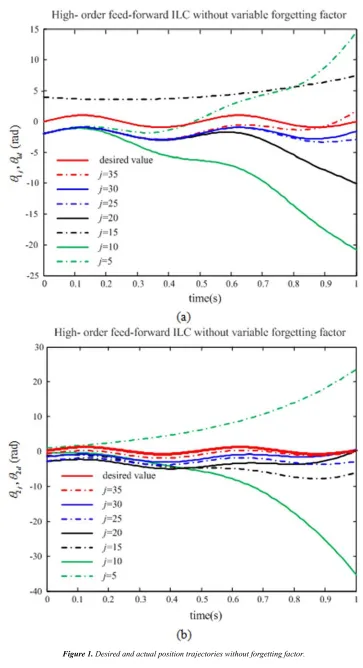
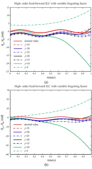
As shown in Figure 1, there is a little larger amplitude of control input in the ILC algorithm without forgetting factor. From Figure 2, we can see that a better tracking performance can be obtained using the high-order feed-forward ILC algorithm with forgetting factor, even in the conditions of uncertainty and non-repetitive disturbance from iteration to iteration. That is attributed to the forgetting factor c, which can weaken the disturbance. But for the feed-forward ILC algorithm without forgetting factor, there are large stable tracking errors.

Figure 3 shows the absolute maximum tracking error from iteration to iteration, although the error curve is not perfectly smooth due to the presence of uncertainty and disturbance. From this figure, we can see that the ILC algorithm with forgetting factor can obtain a very fast convergent rate and very small and monotonic decreased tracking errors. But for the feed-forward ILC algorithm without forgetting factor, although high-order controller is used, the tracking errors were unsatisfactory and more iterations were needed to obtain a relatively acceptable tracking performance. We can see that the tracking errors are still relatively large compared with approach 1. It demonstrated that the forgetting factor is more useful in terms of reducing tracking error and speeding up the convergence.

Figure 4 show the error tracking performance in the last iteration for the two methods. In the last iteration, the maximum position errors of eθ1 and eθ2 were about near zero by using the proposed ILC algorithm with a variable forgetting factor. It should be noted that, while the position and errors tracking performance was improved from iteration to iteration, the control input required to drive the system were nearly the same from iteration to iteration, after the first few iterations. It can be seen from Figures 1 and 2, especially from the 15th iteration onwards to the 30th iteration.

5. Conclusion

This paper addresses the ILC with variable forgetting factor problem for a class of robot manipulator system with time-varying disturbances and unknown uncertain. By introducing the variable forgetting factor, the convergent influence of the system caused by state disturbances is weakened. The update law exploits both predictive and current learning terms to enhance stability characteristics and drives the inputs, states, and outputs to their desired ones within bounds. The simulation results show that the system has excellent trajectory tracking effect. The future work aims to apply the proposed algorithm to actual robot control.

Acknowledgment

This research was financially supported by National Natural Science Foundation of China (Project No. 61473248); Natural Science Foundation of Hebei Province of China (Project No. F2016203496); National Intellectual Property

Office of China (Grant No. ZL-2012-1-0052200.2; Zl-2012-1-0052199.3; Zl-2014-2-0411083.9); and China National Heavy Machinery research institute.

References

[1] D. Best, J. Liu, L. Rene, and R. V. D. Molengraft, "Second-order iterative learning control for scaled setpoints," IEEE Trans. Contr. Syst. Tech., vol. 23, no. 2, pp. 805-812, Mar. 2015.

[2] S. Arimoto, M. Sekimoto, K. Tahara, "Iterative learning without reinforcement or reward for multijoint movements: a revisit of bernstein's DOF problem on dexterity," Journal of Robotics, vol. 2016, Article ID 2016315, pp. 1-11, May. 2016.

[3] T. Abdelhamid, "Adaptive iterative learning control for robot manipulators," Automatica, vol. 40, no. 7, pp. 1195-1203, Jul. 2004.

[4] P. Sampson, C. Freeman, S. Coote, and S. Demain,“Using functional electrical stimulation mediated by iterative learning control and robotics to improve arm movement for people with multiple sclerosis,” IEEE Trans. Neur. Syst. Reh., vol. 24, no. 2, pp. 235-248, Feb. 2015.

[5] C. Li, L. Chang, Z. Huang, Y. Liu, and N. Zhang,"Parameter identification of a nonlinear model of hydraulic turbine governing system with an elastic water hammer based on a modified gravitational search algorithm," Eng. Appl. Artif. Intel., vol. 50, pp. 177-191, Apr. 2016.

[6] H. Q. Sun, and A. G. Alleyne, "A computationally efficient norm optimal iterative learning control approach for LTV systems," Automatica, vol. 50, no. 1, pp. 141-148, Jan. 2013. [7] A. Tayebi, and C. J. Chien, "A unified adaptive iterative

learning control framework for uncertain nonlinear systems," IEEE Trans. Autom. Control, vol. 52, no. 10, pp. 1907-1913, Oct. 2007.

[8] K. L. Moore, Y. Q. Chen, and V. Bahl, "Monotonically convergent iterative learning control for linear discrete-time systems," Automatica, vol. 41, no. 9, pp. 1529-1537, Sep. 2005.

[9] D. Huang, J. X. Xu, V. Venkataramanan, and T. C. T. Huynh, "High-performancetracking of piezoelectric positioning stage using current-cycle iterative learning control with gain scheduling," IEEE Tans. Indus. Electr., vol. 61, no. 2, pp. 1085-1098, Feb. 2014.

[10] X. Bu and Z. Hou, “Adaptive iterative learning control for linear systems with binary-valued observations,” IEEE Trans. Neur. Net. Lear., vol. 99, pp. 1-6, Nov. 2016.

[11] J. Zhou, H. Yue, J. Zhang, and H. Wang, “Iterative learning double closed-loop structure for modeling and controller design of output stochastic distribution control systems,” IEEE Tans. Contr. Sys. Tech., vol. 22, no. 6, pp. 2261-2276, Nov. 2014.

[13] G. Pipeleers, and K. L, “Moore reduced-order iterative learning control and a design strategy for optimal performance tradeoffs,” IEEE Trans. Autom. Control, vol. 57, no. 9, pp. 2390-2395, Sep. 2012.

[14] X. Jin, “Adaptive iterative learning control for high-order nonlinear multi-agent systems consensus tracking,” Syst. Control Lett., vol. 89, pp. 16-23, Mar. 2016.

[15] A. Luo, X. Xu, L. Fang, and H. Fang, “Feedback-feedforward pi-type iterative learning control strategy for hybrid active power filter with injection circuit,” IEEE Trans. Ind. Electron., vol. 57, no. 11, pp. 3767-3779, Nov. 2010.

[16] Z. Li, Y. Hu, and D. Li, “Robust design of feedback feed-forward iterative learning control based on 2D system theory for linear uncertain systems,” Int. J. Syst. Sci., vol. 47, no. 11, pp. 2620-2631, Aug. 2015.

[17] C. Paleologu, J. Benesty, and S. Ciochina, “A robust variable forgetting factor recursive least-squares algorithm for system identification,” IEEE Signal Proc. Let., vol. 15, pp. 597-600, Oct, 2008.

[18] K. Zhang, C. R. Zhao, and X. J. Xie, “Global output feedback stabilisation of stochastic high-order feed forward nonlinear systems with time-delay,” Int. J. Control, vol. 88, no. 12, pp. 2477-2487, Dec. 2015.

[19] R. M. Canetti and M. D. España, “Convergence analysis of the least-squares identification algorithm with a variable forgetting factor for time-varying linear systems,” Automatica, vol. 25, no. 4, pp. 609-612, Jul. 1989.

[20] Z. Zhong, Y. Zhu, and T. Yang, “Robust decentralized static output-feedback control design for large-scale nonlinear systems using takagi-sugeno fuzzy models,” IEEE Access, vol. 4, pp. 8250-8263, Nov. 2016.

[21] W. Paszke, S. Hao, K. Galkowski, and T. Liu, “Robust iterative learning control for batch processes with input delay subject to time-varying uncertainties,” IET Control Theory Appl., vol. 10, no. 15, pp. 1904-1915, Oct. 2016.

[22] L. Lu, H. Zhao, and B. Chen,

“Improved-variable-forgetting-factor recursive algorithm based on the logarithmic cost for volterra system identification,” IEEE Trans. Circuits-II, vol. 63, no. 6, pp. 588-592, Jun. 2016.