21
ADJUSTMENT DYNAMICS BETWEEN ALTERNATIVE ASSET CLASSES: GOLD, RUPEE
& CRUDE USING ARDL BOUNDS TESTING APPROACH
Namrata Chaubey & Apurva Gupta
Student BMS, Bhim Rao Ambedkar College, University of Delhi,
Dr. Rakesh Shahani
Associate Professor, Bhim Rao Ambedkar College, University of Delhi (corresponding author)
Abstract
The paper investigates short and long term linkages between Movement of Gold, Oil and Rupee in India; the three popular alternative asset classes. The methodology used for this purpose has been Autoregressive Distributed Lag (ARDL) Bounds Testing Approach. To test this hypothesis of co-integration between alternative asset classes, we have analyzed log transformed monthly returns for these alternate asset classes for the ten year period i.e. April 1, 2005 -March 31, 2015. The econometric techniques used in our study include the Unit Root ADF , (for stationarity testing of variables) , Akaike Information Criteria (AIC) for determining the optimal lag length of our model, Breusch Godfrey –Lagrange Multiplier Test (for detecting Serial Correlation) & Cumulative Sum of Recursive Residuals (CUSUM) Test ( for Stability of our parameters). For detecting the Long term relation we have used partial ‘F’ test with critical values as given by Pesaran, M. H., Shin, Y. &Smith ,R. J. (2001). The short term and long term linkages have been established using the Error Correction Model after generating error correction term from the co-integrating vector.
The results of the study reveal that all our variables are stationary at I(1) Level, which is also one of the pre requisite for our ARDL Bounds test . Further the best model as identified by AIC is lag(1) for all the three regressions. The ‘F’ Bounds test could establish co-integration and long term relation only when crude taken as a function of other two variables namely rupee and gold. All the three variables were found to be stable when CUSUM test was employed .
Introduction
In today’s time when anyone talks of financial markets, the immediate picture which comes to our mind is that of stock markets. On the other hand those who have the knowledge of these markets are also aware of asset classes which serve as alternate to stock markets, and these include assets like Crude Oil & Gold, both of which belong to the commodity asset class. We also have another alternate asset class; the Indian Rupee which is also gaining popularity amongst the investors, however unlike gold and oil it does not belong to commodity asset class.
The stock markets have also been one of the most preferred segment of research for analysts over the years. The reason for the same is quite evident, the ease of availability of information about the stock prices . One of the commonly researched are here is to study the inter linkages between stock markets with the intention to test the Causal Relation, their Co-movement /& co-integration between markets (e.g. Stock Indices of Different Countries)
(Mahajan A et al 2014, Garg Vaibhav et al. 2012 etc.)
On the other hand when we talk of research on alterative asset classes, this too has also closely been associated with stock markets & on most occasions research has been in conjunction with the stock markets e.g. movement or commodities viz. a. viz. equities , studying the spillover effect from stock market to currency market, (this area of spillover has actually gained much importance particularly after the East Asian Crisis of 1997 when the world witnessed a collapse of almost all the financial markets. (Bagchi Bhaskar 2014)).
On the other hand there have been only a handful of studies where the focus has been to study the movement only from the group of alterative asset classes. This is mainly because each alternate asset class has been traditionally been influenced by a set of factors which do not affect other alternate asset classes. However since financial markets are unpredictable , the last financial crisis saw a remarkable co-movement of these alternate asset classes and moreover post financial crisis the frequency of these co-movements have increased dramatically.
22
new approach (ARDL) which has been followed has four major advantages over traditional approaches of co-integration, first it can be applied to small samples, second it avoids the omitted variable bias by estimating short and long run relationship simultaneously , third the precondition stationarity of variables is restricted to I(0) & I(1) and not higher and moreover the variables need not be normal , fourthly after determining the appropriate lag length, a simple multiple OLS regression is required & the last advantage is that the test can be applied even if some of the regressors are endogenous (Srinivasan, P., &Prakasam, K. (2014))
Review of Literature
The focus of this section is to examine some of those studies where the new co-integration methodology (ARDL) Bounds Testing Approach has been applied. The section also reviews the existing research on some of the alternate asset classes.
Joshi, P., &Giri, A. K. (2015) examined short & long run relationship between Indian stock prices & India’s macroeconomic variables for approx. ten year period April 2004-July 2014. The methodology used was ARDL bounds approach to co-integration. This was followed by Error Correction Model & Variance Decomposition Analysis . The results of the study showed a long run co-integrating relationship between the variables. A view on some of the macro economic variables showed that IIP, inflation and USD-Rupee exchange rate influenced stock prices in a positive manner whereas price of gold influenced the stock prices in opposite direction. The error correction indicated long run causal relation running from all the variables to stock prices. Variance decomposition showed that own shocks were more powerful than outside shocks. Shahani R, YashGarg & Ankita Sharma (2015) researched gold and oil as the two alternative asset classes for their relation using statistical tools including Granger Causality, Engle-Granger Co-integration & VECM. The results from the study failed to justify any cause effect relation between the two asset classes ;co-integration was however proved . Error Correction Model could also detect long term equilibrium. Srinivasan, P., & Prakasam, K. (2014)tested for monthly data (June 90 to April 14), ADRL Bounds test for testing the causal linkages between stock prices, gold & USD Rupee exchange rate. The results showed that gold & stock prices showed long-run relationship with USD Rupee rate. On the other hand long- run co-integration between stock price &gold price could not be proved by the study. The results further researched the cause effect relation and found no causality between the above two variables. MahajanAanchal, PriyashaSaluja& RakeshShahani (2014) made a study of Indian Market viz. a. viz. other BRICS Markets for a ten year period ; 2003-2013 & found that the only one market from BRICS , the Russian Market was impacting or having cause effect relation with India while the same could not be proved by studying other markets Afzal, M., Malik, M. E., Butt, A. R., & Fatima, K. (2013)used ARDL bounds approach to examine the relation between inflation & openness in Pakistan. The period of study was from 70-71 to 08-09. The results showed short run inverse linkages between the variables with two way causal relation also being established in the study Ahmed, M. U., Muzib, M., & Roy, A. (2013) explored the relation between CPI and wages during the period 1975-76 to 2009-10 using ARDL bound testing approach. Other macro determinants used in the study included exchange rate of Takka with US dollar, credit (domestic) & GDP. The study showed domestic credit &nominal wage rate were positively related to price level in the short-run as well as long run. The long-run relation between price &other variables was also proved. Gaikwad, P. S., &Fathipour, G. (2013) made an attempt to analyze the FDI flows to India on GDP growth. The methodology used was ARDL method , period of study was 1990-2008. The results of the study showed long run relation among the growth of GDP & its determinants &that FDI had a positive significant impact on GDP.
Shahani Rakesh, GargVaibhav, Jatin Thakkar & Shubham Tandon (2013) used daily return data (Oct 1, 2010-Sep 30, 2012) to fit an Error Correction Model to determine the short & long term linkages between BSE Sensex & US (DJIA) ,Germany’s DAX and France CAC stock prices. The results of the study showed coefficient to be negative with a move back towards long run equilibrium. The results also showed impact of European Markets to be more on India than was that of US Markets. Srinivasan, P., & Kalaivani, M. (2012) investigated the effect of volatility of exchange rate on India’s real exports using the ARDL bounds test approach The data for the study was for the period 1970 to 2011. The results of the study showed real exports to be co-integrated with all the variables namely volatility of exchange rate, exchange rate(real)&GDP. The results showed GDP had a long run positive & significant, but short run insignificant effect on India’s real exports. The exchange rate volatility was found to be negative (but was significant ) on real exports , this result was obtained for both short& long run; further the real exchange rate was found to have negative short but positive long run impact on real exports.
23
Data and Methodology Adopted
The period of study has been taken to be monthly figures for ten year period i.e. April 1st2005 to March31st 2015. The
data sources include websites of Yahoo Finance (in. finance. yahoo.com), www.macrotrends.net, www.investing.com & www.bseindia.com. The statistical tools which have been applied in our study include (a) ADRL Bounds Partial ‘F’ Test (b)Wald Test for Joint significance of Hypothesis (c) Augmented Dickey Fuller (ADF) test of Stationarity of Variables (d) AIC & SIC Optimal Lag Length Criteria (e) Breusch Godfrey –Lagrange Multiplier Test (for detecting Serial Correlation) (e) CUSUM Test for Stability of parameters.
(i) Testing the Stationarity of Variables
We apply ADF test (with intercept and trend) to find out the stationarity of our three variables; Gold, Crude Oil and Rupee. We use the following equations (i to iii) for this purpose.
Δ Crude t =β1 + (β2 – 1)Crude t -1+ Δ Crude t -i + u1t …… eq(i)
Δ Gold t =α1 + (α 2 – 1)Gold -1 + Δ Gold t -i + u2t … eq(ii)
Δ Rupee t =θ1 + (θ2 – 1)Rupee t -1+ θ Δ Rupee t -i + θ u3t …… eq(iii)
(For the equation (i) ; The variable for which we are testing stationarity is Crude . Δ Crude t is change in Crude in period t, (β2 –
1) is the coefficient of the Stationarity for variable , Δ Ret Crude t -i denotes change in Crude in period t-i & is the
augmented variable which has been added to take care of autocorrelation and the term adds up ‘m’ times till the autocorrelation is removed , is the trend variable and takes care of deterministic trend in the variable so that only stochastic trend can be detected, the u 1t is random error term. Similarly we carry out stationarity tests (eq(ii) & eq(ii)) for other two variables namely
the gold and rupee )
The testable hypothesis (H0) for our Stationarity test of our Variable Crude ( eq (i)) would be
β2 – 1 =0 0r β2 = 1 (the crude is not stationary )
Alt Hyp (Ha): β2 – 1 ≠0, (crude is stationary)
(ii) ADRL Bounds Test
We first determine the long term relation/co-integration between our variables namely crude, , rupee and gold . For this we develop the following equations (iv to vi see below) by take the first difference of the dependent variable(say variable 1) and lags of all the variables as independent and first lag of all the variables as independent . This is a long run relation. However we usually write our ARDL Model to include short term relation also i.e. the regression is a combined one to include short run and long run simultaneously
Next we undertake joint testing of the Null of No Co-integration : Ho1 : β2= β3= β4= 0 & apply partial ‘F’
test . The ‘F’ computed is compared with critical at 5 % level ; 3.79 (lower bound level at I (0) & 4.85 (as upper bound level at I (1))(these levels have been obtained from Pesaran, M. H., Shin, Y., & Smith, R. J. (2001)). The criteria for co-integration is to accept the Null, if ‘F’ computed< Lower Bound critical & if ‘F’ computed> Upper Bound critical , reject the null or
co-integration is established . If F Computed is between the two bounds , inference is in conclusive.
ΔY1,t = 1+ 2 Y 1,t-1+ 3 Y 2,t-1 + 4 Y 3,t-1+ Δ
+ + Δ + Δ +u1t
….(iv) ,
ΔY2,t= 1+ 2 Y 1,t-1+ 3 Y 2,t-1 + 4 Y 3,t-1+ Δ
+ + Δ + Δ +u2t
……….(v) ,
ΔY3,t = 1+ 2 Y 1,t-1+ 3 Y 2,t-1 + 4 Y 3,t-1+ Δ
+ + Δ + Δ +u3t
24
(Note: Y1t, Y2t Y3t represent the three variables namely crude, rupee, gold. ‘i’ is the no. of lags and all the lags for each of our
lagged variables are summed up till ‘n’ depending upon the AIC/SIC optimal lag length obtained, say for it would imply
that different betas are computed for lags of variable , as i goes from 1 to ‘n’ .For selecting the most optimal model we
apply the AIC Criteria )
(iii) Data Diagnostics
(a) Presence of Serial Correlation
Under this we check for serial correlation for each of our variables & the test used is Breusch Godfrey – Lagrange Multiplier Test. Consider autoregressive equation of any variable (say Gold), we start by obtaining the residuals i.e.
Yt = 1+ 2 Yt-1 + 3 Y t-2 + ……+ p Y t-(p-1) + ut……….(vii),
(‘p’ is the no. of lags in the regression, we may say this is also the order of coefficient of lagged regression)
Further let the residuals ut follow the following structure:
ut = ρ1 ut-1 + ρ2 u t-2 + ρ3 u t-3 + ……+ ρm u t-m + et ……….(viii)
(BG LM test assumes ‘p’ > ‘m’)
Next we define our Null as: ρ1=ρ2= ρ3 =…. ρm= 0
To carry out the BG Autocorrelation test we run the following equation (eq ix)
ut = 1+ 2 Yt-1 + 3 Y t-2 + ……+ p Y t-p + ρ1 ut-1 + ρ2 u t-2 + ρ3 u t-3 + ……+ ρm u t-m + et ……….(ix)
The above equation (ix) is a combined equation of (vii) & (viii) & our objective is to determine the R Square of combined equation which follows Chi Square Distribution. We reject the Null of No autocorrelation if R2(n-p) > χ2m.
(See Gujarati N. Damodar and Sangeetha, Basic Econometrics, 4th edition, Tata McGraw Hill Education Pvt. Ltd.2007)
(b) Stability of the Model
This test is called Cumulative Sum of Recursive Residuals test (CUSUM) where we cumulate the residuals for each time period of study. Next we a plot of this cumulative sums (‘y’ axis) against the period of study (‘x’ axis) , the moment this cumulative sum value at any period falls outside the limit μ ±2 SE i.e. (5 %level), the model stability is breached
(iv) Error Correction Term
If the long run co integration is established through above ‘F’ test from ARDL Bounds Test point (ii) above , next is to obtain the ECM error term , for which we run the usual equations by taking one variable as the function of other two variables and obtain the residuals which are then lagged to obtain lagged residuals i.e.u1t-1 ,u2t-1 & u3t-1
(a) Y1,t = 1+ 2 Y 2,t + 3 Y 3,t + u1,t ……….(x) (b) Y2,t = 1+ 2 Y 1,t + 3 Y 3,t + u2,t ……….(xi) (c) Y3,t = 1+ 2 Y 1,t + 3 Y 2,t + u3,t ……….(xii)
(v) Obtain short term parameters & coefficient of the lagged error term
The lagged error term variable obtained from (v) above is combined with variables for the short term and the following regressions (xiii, xiv & xv) are estimated.
ΔY1,t = α 1+ α 2 u1,t-1 + Δ + + Δ + Δ + e1,t….….(xiii)
ΔY2,t = α 6+ α 7 u2,t-1 + Δ + + Δ + Δ + e2,t ….(xiv)
25
(Where ψ, γ & θ are the short run parameters to be estimated, α 2, α 4& α 6 are the parameters of error correction term(ECM) terms
u1,t-1 u2,t-2 , u3,t-1 obtained from the co-integrating vector (Step iii). It is to be noted that ‘n’ for the short term co-integration shall
be defined by the best model as given by AIC/SIC.)
Results and Inferences of the study
The appendices gives the results of the study in a tabular format.. To begin with Table 1 in appendix discusses the results of the stationarity of our variables ; this is a pre-requisite for the ARDL Test and the results clearly show that all our variables are I(1) Stationary as Computed ‘t’ > Dickey Fuller Table ‘t’ Value.
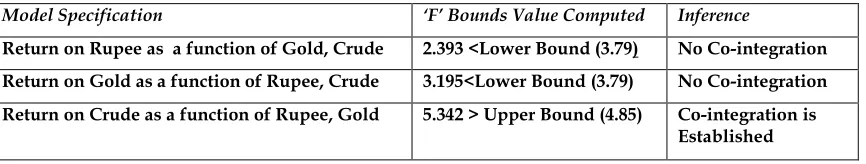
Having established the stationarity of our variables we now proceed to check for Co-integration using Partial ‘F’ Bounds approach. The results are given in Table 2 in appendix as Partial‘F’ Test Result. The results show that Co-integration is established only when Crude is a function of other two variables namely gold and oil while no co-integration could be established for other two relations.
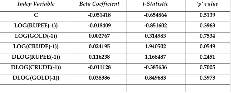
Results of three equations developed under ADRL showing long run dynamics between the three variables gold, crude and rupee are given in Table 3,4 & 5 in appendix. The lag value has been restricted to one lag as determined by AIC & SIC . The details of AIC & SIC using different lags for our variables is shown in Table 6 in appendix.
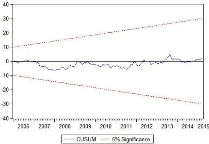
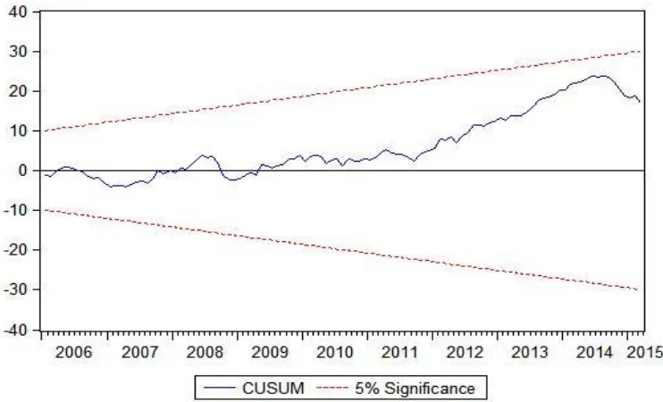
In the next part of our analysis , we established the serial correlation BG-LM test for three variables namely Gold , Rupee & Crude. The results showed Gold (‘F’ = 3.68 , Prob ‘F’ =0.07),Crude(‘F’ = 4.8 ,Prob ‘F’=0.043) Rupee (‘F’ = 5.13, Prob ‘F’=0.028). We also established the stability of our three variables using CUSUM test, the results are shown in Fig (i),(ii) & (iii). These results show that all our variables are stable as the CUSUM line is within the upper and lower limits of 5 %.
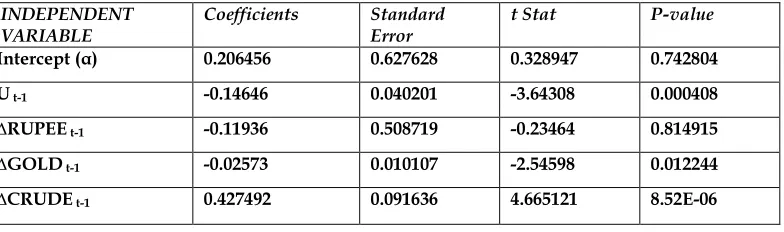
In our final analysis, we established the short run equilibrium and also error correction between the long and short run (Table 7(i), (ii) & (iii) in appendix) . The coefficient of the lagged error term which shows that speed of adjustment between dynamics of short and long run is negative in all the three equations; however it was significant only for the equation: crude as a function of rupee and gold. The interpretation of the error term variable for this coefficient whose value is -0.1464 shows that there would be an adjustment backwards and in one period the adjustment factor is 14.6 %.
Conclusion
The study investigated using ARDL Bounds Approach the short and long term linkages between Movement of Gold, Oil and Rupee in India for the ten year period i.e. April 1, 2005 -March 31, 2015. The three ARDL regressions were tested for optimality using AIC, for serial correlation using Breusch Godfrey –Lagrange Multiplier Test , for stability using CUSUM Test, for establishing long term stability using partial ‘F’ test, for short term and long term linkages using Vector Error Correction.
The results showed co-integration and long term relation was established only with crude as a function of other two variables namely rupee and gold while the same could not be established for rest of the equations . Further all our variables were stationary at I(1) & the best model as identified by AIC was with lag(1) for all the three regressions. Further all the variables were stable as shown by CUSUM plots.
References
Afzal, M., Malik, M. E., Butt, A. R., & Fatima, K. (2013). Openness, inflation and growth relationships in Pakistan: An application of ARDL bounds testing approach. Pakistan Economic and Social Review, 51(1), 13.
Ahmed, M. U., Muzib, M., & Roy, A. (2013). Price-Wage Spiral in Bangladesh: Evidence from ARDL Bound Testing Approach. International Journal of Applied Economics, 10(2), 77-103.
Bagchi, Bhaskar. (2014) Causality between liquidity management & profitability: Evidence from Indian CPSEs International Journal of Services and Operations Management, Vol.18(2), pp212-232.
Gaikwad, P. S., & Fathipour, G. (2013).The Impact of Foreign Direct Investment (FDI) on Gross Domestic Production (GDP) in Indian Economy.Information Management and Business Review, 5(8), 411.
Garg Vaibhav, JatinThakkar, ShubhamTandon and Rakesh Shahani( 2012) Recent Trends in Causality : The Impact of European Markets Paper Presented at an International Seminar on Economic Social and Environmental Challenges of Globalization Organized by St. Bede's College Shimla Oct 5-6
Gujarati N. Damodar and Sangeetha, Basic Econometrics, 4th edition, Tata McGraw Hill Education Pvt.
Ltd.2007
26
Kamaruddin, R., &Masron, T. A. (2010). Sources of growth in the manufacturing sector in Malaysia: Evidence from ARDL and structural decomposition analysis. Asian Academy of Management Journal, 15(1), 99-116.
Mahajan A, Priyasha Saluja & RakeshShahani (2014)Does the popular BRICS Model reflect a contagion effect’ paper presented at 2nd International Conference “India 2020: Vision For The Financial Sector” Sri Guru
Gobind Singh College of Commerce, Delhi, March 10-11.
Pesaran, M. H.& Shin, Y (1999) An autoregressive distributed lag approach to co-integration analysis, Centennial Vol of Ragnnar Frisch ed, , Strom A , Cambridge University Press, UK
Pesaran, M. H., Shin, Y., & Smith, R. J. (2001).Bounds testing approaches to the analysis of level relationships. Journal of applied econometrics, 16(3),pp 289-326.
Shahani R, YashGarg&Ankita Sharma (2015) Adjustment Dynamics in Causal Linkages between Oil &Gold : An Empirical Investigation International Conference on Evidence Based Management : BITS Pilani, March. Excellent Publishing House , Rajasthan
ShahaniRakesh (2012) ‘Causality between Sensex and Dow: Sub Prime and Beyond’ Paper Presented at Sixth National Seminar on Capital Markets, IBS, Gurgaon, March 2-3.
Shahani Rakesh,GargVaibhav, JatinThakkar&ShubhamTandon (2013) Modeling Equilibrium Relation between market returns of the US, European and Indian Markets through ECM and Co-integration Approaches, Indian Capital Markets: An Empirical Analysis , ICFAI University Press, Hyderabad
Shittu, O. I., Yemitan, R. A., &Yaya, O. S. (2012). On Autoregressive Distributed Lag, Cointegration And Error Correction ModeL [An Application to Some Nigeria Macroeconomic Variables,. Australian Journal of Business and Management Research, 2(8), 56.
Srinivasan P. and Karthigai, P. (2014), Gold Price, Stock Price and Exchange Rate Nexus: The Case of India, The IUP Journal of Financial Risk Management, 11(3), 1-12.
Srinivasan, P., & Kalaivani, M. (2012). Exchange Rate Volatility and Export Growth in India: An Empirical Investigation. MPRA Paper, (43828).
Websites: in.finance.yahoo.com, www.macrotrends.net, www.investing.com & bseindia.com
Appendices
Table 1 :Regression results for testing stationarity of our variables
VARIABLE N
COEFFICIENT
β2-1 SE(β2-1) |tcal|
|ttable|
DICKEY FULLER
STATIONA RY I(0) or
I(1)
RUPEE 119 -0.87644702 0.092161391 9.50992 2.89 I(1)
CRUDE 119 -0.650119696 0.086976442 7.474665 2.89 I(1)
GOLD 119 -1.151385212 0.091571385 12.57363 2.89 I(1)
Table 2 : ARDL Co-integration Partial ‘F’ test Results
Model Specification ‘F’ Bounds Value Computed Inference
Return on Rupee as a function of Gold, Crude 2.393 <Lower Bound (3.79) No Co-integration Return on Gold as a function of Rupee, Crude 3.195<Lower Bound (3.79) No Co-integration Return on Crude as a function of Rupee, Gold 5.342 > Upper Bound (4.85) Co-integration is
Established
Table 3: ARDL Model results for rupee as a function of Crude Oil & Gold (optimal model by AIC Criteria: one lag)
27
Indep Variable Beta Coefficient t-Statistic ‘p’ value
C -0.051418 -0.654864 0.5139 LOG(RUPEE(-1)) -0.018409 -0.851602 0.3963 LOG(GOLD(-1)) 0.002767 0.314983 0.7534 LOG(CRUDE(-1)) 0.024195 1.940502 0.0549 DLOG(RUPEE(-1)) 0.116238 1.168487 0.2451 DLOG(CRUDE(-1)) -0.011128 -0.385636 0.7005 DLOG(GOLD(-1)) 0.038386 0.849683 0.3973
Table 4 : ARDL Model results for Crude Oil as a function of rupee and gold (optimal model by AIC Criteria: one lag)
Dependent Variable :∆ln Crude Oilt; (DW : 2.108)
Indep Variable Beta Coefficient t-Statistic ‘p’ value
C 0.787998 3.109004 0.0024 LOG(RUPEE(-1))* -0.148439 -2.127185 0.0356 LOG(GOLD(-1))* 0.063882 2.252625 0.0262 LOG(CRUDE(-1))* -0.148577 -3.691493 0.0003 DLOG(RUPEE(-1)) 0.004745 0.014775 0.9882 DLOG(CRUDE(-1))* 0.445525 4.782990 0.0000 DLOG(GOLD(-1))* -0.360616 -2.472802 0.0149
* Coefficient Significant at 5 % level
Table 5 : ARDL Model results for gold as a function of Crude Oil &rupee (optimal model by AIC Criteria: one lag)
Dependent Variable :∆ ln gold t(DW : 2.02)
Indep Variable Beta Coefficient t-Statistic ‘p’ value
C 0.488288 2.886483 0.0047 LOG(RUPEE(-1)) -0.070845 -1.521127 0.1311 LOG(GOLD(-1)) -0.008697 -0.459493 0.6468 LOG(CRUDE(-1)) -0.032151 -1.196848 0.2339 DLOG(RUPEE(-1)) -0.281607 -1.313930 0.1916 DLOG(CRUDE(-1)) -0.037472 -0.602738 0.5479 DLOG(GOLD(-1))* -0.226287 -2.324881 0.0219
28
Table 6 : Optimal Lag determination for our ARDL Models with rupee, gold and crude as three dependent variables in three models
Dep Var. : ∆Rupee │Dep Var.: ∆Gold │Dep Var.:∆ Crude
No. of Lags AIC SC AIC SC AIC SC
Lag 6 -4.427 -3.896 -2.710 -2.179 -1.982 -1..451 Lag 5 -4.417 -3.961 -2.748 -2.291 -2.009 -1.553 Lag 4 -4.447 -4.065 -2.800 -2.650 -2.021 -1.640 Lag 3 -4.435 -4.144 -2.886 -2.418 -2.044 -1.736 Lag 2 -4.448 -4.212 -2.886 -2.418 -2.075 -1.839 Lag 1 -4.455 -4.290 -2.919 -2.479 -2.111 -1.946
29
Fig 2 :CUSUM (Stability ) test for the residuals of our Model II with gold as dependent variable
30
Table 7(i) Regression results for Error Correction and Short run integration DEPENDENT VARIABLE :∆ RUPEEt
INDEPENDENT
VARIABLE Coefficients Standard Error t Stat P-value
Intercept (α) 0.125365 0.1239 1.011825 0.313783 u t-1 -0.0175 0.021382 -0.81833 0.414891
∆RUPEEt-1 0.130864 0.099271 1.31826 0.190083
∆GOLD t-1 0.001618 0.002014 0.803677 0.423271
∆CRUDE t-1 0.001371 0.017632 0.077749 0.938165
Table 7(ii) Regression results for Error Correction and Short run integration DEPENDENT VARIABLE:∆ GOLDt
Table 7 (iii) Regression results for Error Correction and Short run integration DEPENDENT VARIABLE:∆CRUDE
OILt
INDEPENDENT
VARIABLE Coefficients Standard Error t Stat P-value
Intercept (α) 0.206456 0.627628 0.328947 0.742804 U t-1 -0.14646 0.040201 -3.64308 0.000408
∆RUPEE t-1 -0.11936 0.508719 -0.23464 0.814915
∆GOLD t-1 -0.02573 0.010107 -2.54598 0.012244
∆CRUDE t-1 0.427492 0.091636 4.665121 8.52E-06
INDEPENDENT
VARIABLE Coefficients Standard Error t Stat P-value
Intercept (α) 9.386408 6.143078 1.527965 0.129316
U t-1 -0.00213 0.021699 -0.09811 0.922021
∆RUPEEt-1 -8.32215 4.915973 -1.69288 0.093234
∆GOLDt-1 -0.24287 0.099452 -2.44203 0.016155