Reliability Analysis with Dynamic Reliability Block Diagrams in the Möbius Modeling Tool

Reliability Analysis with Dynamic Reliability Block

Diagrams in the Möbius Modeling Tool

Ken Keefe

University of Illinois at Urbana-Champaign Urbana, Illinois, USA

[email protected]

William H. Sanders

Department of Electrical and Computer Engineering

University of Illinois at Urbana-Champaign Urbana, Illinois, USA

[email protected]

ABSTRACT

Reliability block diagram (RBD) models are a commonly used reliability analysis method. For static RBD models, combinatorial solution techniques are easy and efficient. How-ever, static RBDs are limited in their ability to express vary-ing system state, dependent events, and non-series-parallel topologies. A recent extension to RBDs, called Dynamic Re-liability Block Diagrams (DRBD), has eliminated those lim-itations. This tool paper details the RBD implementation in the M¨obius modeling framework and provides technical details for using RBDs independently or in composition with other M¨obius modeling formalisms. The paper explains how the graphical front-end provides a user-friendly interface for specifying RBD models. The back-end implementation that interfaces with the M¨obius AFI to define and generate exe-cutable models that the M¨obius tool uses to evaluate system metrics is also detailed.

Categories and Subject Descriptors

C.4 [Performance of Systems]: Reliability, availability, and serviceability; B.8.1 [Performance and Reliability]: Reliability, Testing, and Fault-Tolerance

Keywords

Reliability Modeling, Availability Modeling, Continuous Time Markov Chain Models, State-based Reliability Model, M¨obius Atomic Model Formalism

1.

INTRODUCTION

Reliability analysis is an essential part of critical system de-sign and planning. Many methods exist to support such analysis, such asreliability block diagrams(RBD),fault trees, andreliability graphs [6][11]. These methods work well for limited cases.

However, those methods do not offer a way to handle dy-namic behavior, such as how the failure of one component

impacts the behavior of the remaining elements. Common notions in system design, such as complex redundancy mod-els (e.g., cold spares, warm spares, hot spares) and load bal-ancing, are also not available in those approaches.

Dynamic Reliability Block Diagrams (DRBDs) [2] are a re-cent development that expands on reliability block diagrams to address those issues. DRBDs add model state to tradi-tional RBDs to support dynamic change of component state over time. Adding state and time enables the use of state dependent expressions to offer time-dependent, rich redun-dancy, and load-balancing behaviors.

The primary contribution of this paper is a detailed discus-sion of a new implementation of the Dynamic Reliability Block Diagram formalism within the M¨obius tool. Section 2 provides an introduction to reliability block diagrams and Dynamic Reliability Block Diagrams.

The M¨obius modeling tool leverages a framework that en-ables multiple modeling formalisms, including compositional formalisms that flexibly connect multiple, diverse models into a single model. The framework provides several solu-tion techniques, such as simulasolu-tion and analytical solusolu-tion to solve for metrics that are defined on the model. M¨obius uses a well-defined abstract functional interface (AFI) [3] to allow for the addition of new modeling formalisms that can leverage the existing experimental and solution methods.

The remainder of this paper is organized as follows, Section 3 describes our implementation of DRBDs in the M¨obius framework. Section 4 explains how the RBD formalism can be used effectively in M¨obius. Section 5 details related tools that work with DRBDs or similar reliability models. Section 6 concludes the paper.

2.

FORMALISM DEFINITION

The RBD formalism implemented by this work is very sim-ilar to the original dynamic reliability block diagram con-cept. To understand the subtle differences, we begin with our interpretation of the RBD formalism and then explain the details of the DRBD formalism.

2.1

Reliability Block Diagrams

RBDs offer a graphical representation of the reliability re-lationship of system components that expresses the overall system reliability. System analysts can easily define and

VALUETOOLS 2015, December 14-16, Berlin, Germany Copyright © 2016 ICST

read RBDs.

Each RBD contains a start node, a stop node, a set of block elements that correspond to components in a system that independently fail at some rate, and connections that de-fine the reliability relationship between the components and the system. When a component fails, its block becomes dis-abled. In order for a system to be considered operational, there must be at least one path through the RBD (from start to stop) that does not cross through a disabled block.

The diagram topology of an RBD can typically be decom-posed into two connection classes:

• Series connections indicate a logical ORrelationship. If any of the components in the serial connection fail, the entire system fails.

• Parallel connections indicate a logicalAN D relation-ship. If all of the components in the parallel connection fail, the entire system fails.

Direct combinatorial methods are available for evaluating the system reliability (or availability, if repair is defined) if the diagram is series-parallel, and the failure (and repair) rates are independently distributed.

2.2

Dynamic Reliability Block Diagrams

A Dynamic Reliability Block Diagram is a pair (C,N). C is the set of components in the system. A component is a triple (S,F, R). S is the current state of the component, either Active or F ailed. F and R are failure and repair events, respectively. Each component event is a triple (T, E,R). T is a state-based timing distribution. For example, a web server may fail at a faster rate if several other web servers in a load-balancing configuration have failed, as the traffic will spill over to the remaining web servers. E is the enablement of the event, eithertrueorf alse. R is the resulting effects of the event executing. A component event is enabled based on itsEandS. For example, a component in theF ailedstate cannot fail again, so the failure event is disabled. TheRexpressions are able to update the state of other components. For example, the failure of a repair robot may disable theRepairevents on several components in a system.

N is the set of nodes that represent directed connections among components in the diagram. Nmust contain a unique start node and a unique stop node. Nodes can have zero or more incoming component connections and zero or more outgoing component connections. Those connections rep-resent the same reliability relationship as defined in static RBD models. Specifically, the overall system state is con-sidered operational if there exists a path from the start node to the stop node such that each component along the path hasS=Active.

3.

IMPLEMENTATION IN MÖBIUS

The Reliability Block Diagram atomic model formalism in the M¨obius framework implements Dynamic Reliability Block Diagrams as defined in Section 2.2. The implementation

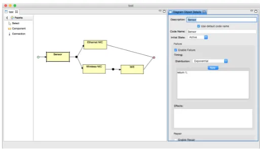
Figure 1: An example of the RBD atomic model editor.

provides a graphical front-end for defining RBD models. RBD model specifications are stored in a textual, XML for-mat. M¨obius uses the RBD implementation to generate C++ code from the XML specification; the code inherits from the formalism-specific, AFI-level C++ code that is part of the implementation and the M¨obius framework.

3.1

RBD Atomic Model Editor

The Reliability Block Diagram atomic model editor is writ-ten in Java and leverages Eclipse libraries to offer a clean and user-friendly interface. The RBD atomic model editor uses the Eclipse Rich Client Platform (RCP) [7], which allows the inclusion of several other useful Eclipse projects. SWT [9] and JFace [5] provide a nice set of native widgets and dialogs. The Eclipse Graphical Editing Framework (GEF) [12] handles the actual drawing and editing of the diagram on a canvas. The Eclipse Modeling Framework (EMF) [15] is a meta-modeling and model code generation engine used widely by Eclipse and Eclipse-related projects. The RBD atomic model implementation uses EMF to define the code models that store a reliability block diagram atomic model. That allows the atomic model to integrate nicely with the existing M¨obius tool. EMF also handles the persistence of RBD models in an XML-formatted file.

Eclipse RCP defines two top-level UI-components, editors and views. For the RBD atomic model editor (Figure 1), a new GraphicalEditorWithFlyoutPalette to handle the palette and diagram canvas was defined, as well as a new ViewPart to allow definition of details of components and nodes.

When a new RBD atomic model is created, a green node and a red node are automatically created and placed on the canvas. They are the start and stop nodes, respectively, of an RBD model. They cannot be deleted, but they can be moved if the default starting position is inconvenient.

On the left side of the editor window is a palette containing a selection tool, an add component tool, and an add con-nection tool. These tools are used to create and change an RBD diagram on the drawing canvas. These tools work as expected, with the exception of the connection tool which will be explained next.

be selected first, followed by the target component. When two previously unconnected components are connected, a new node is created along the path. These nodes are drawn as small black circles and make it possible to have multi-ple sources and multimulti-ple targets for each connection. The importance of nodes will be discussed in Section 3.3. Ad-ditional components can be added to the connection by fol-lowing the above procedure and connecting the component directly to the node itself, or by connecting a component to another component already connected by the node’s connec-tion.

For example, in Figure 1, the connections among Sensor, Ethernet NIC, and Wireless NIC can be defined by using the connection tool on Sensor and then Ethernet NIC, fol-lowed by using the connection tool on the node between Sensor and Ethernet NIC and then the Wireless NIC. Al-ternatively, the second connection can be accomplished by using the connection tool on Sensor and then on the Wire-less NIC. Depending on the order of connections made in an RBD model, several nodes may be created and then merged together. In the end, every component can have at most one incoming connection and at most one outgoing connection.

When a component is selected on the canvas, a Details view appears on the right side of the window. It is shown as the rightmost column in Figure 1. In the Details view, the user can defined the name of a component, as well as its code name, which is the C++ object name by which this component can be referenced within any code expression. Both the name and code name must be unique, and the default behavior is for the code name to be automatically generated based on the name. The initial operational state of the component is next chosen as eitherActive orFailed. Below that portion of the Details view, there are sections for defining the fail behavior and the repair behavior. In each section, there is a check box to indicate whether the behavior should initially be enabled. If it is not enabled, this event will not begin firing until the behavior has been enabled and the operational state of the component has been appropriately set (e.g., fail behavior requires the state to be

Active). Next, a timing distribution can be defined from any of the general distributions that M¨obius supports. The timing distribution will be sampled to find the firing time of this behavior’s event. It is important to note that the parameters of the firing distribution can access the model state. For example, a set of load-balancing servers may fail at a faster rate if their workload increases because one of the other servers fails. Lastly, a C++ expression may be provided in theEffectstext box. That code will execute after the component’s state is updated by the fail/repair event. The effects can be used to alter other parts of the model state in a completely custom way. For example, it can be used to define a k of N failure model for several parallel devices by entering code that checks to see how many of its sibling components are still functional and manually fail a separate component block if thekthreshold has been reached.

3.2

Möbius AFI Overview

The M¨obius AFI is a set of base classes that all formalisms must inherit to integrate with the M¨obius framework and tool [3]. These base classes have pure virtual functions, as

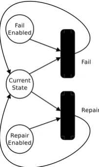
Figure 2: Graphical representation of the state variables and actions that model the failure and repair behavior of a component. Arcs represent preconditions and effects of an action.

defined by the implementation of object-oriented program-ming in C++, that must be defined by derived classes in a formalism. The M¨obius AFI uses these virtual functions to interact in a well-defined manner with the derived classes [3]. The M¨obius AFI defines a base formalism to which every atomic model formalism must provide a mapping. This for-malism containsstate variables andactions. State variables use basic C++ data types to store parts of model state.

TheBaseModelClassdefines a base class that all modeling formalisms must inherit from. A BaseModelClasscontains objects that are state variables and actions that are part of the model. BaseStateVariableClassdefines the C++ class that represents a state variable object in the base formalism. However, a derived class ofBaseStateVariableClass, called SharableSV, can be used to enable the sharing of state vari-ables across different models with varied formalisms. That is an important feature that enables state variable sharing model composition in M¨obius, as explained in Section 4.1.

Actions in the M¨obius AFI define events that change state variable values; those changes transition the model from state to state. An action has an enabling predicate, a firing time distribution (which may be instantaneous), an input function, and an output function. The enabling predicate determines in which model states an action can begin and continue firing. The input and output functions are used to update the model state. BaseActionClassis the base class for all actions in M¨obius.

3.3

RBD AFI Implementation

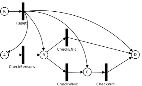
Figure 3: Graphical representation of the state variables and actions that represent the paths of the example model seen in Figure 1. The state variables and actions for component failure and repair have been omitted for clarity. Arcs repre-sent preconditions and effects of an action.

TheRBDModelalso contains a set of ComponentFailaction objects, a set of ComponentRepair action objects, a set of CheckComponentaction objects, and a single ResetPathEx-plorationaction object. All actions in an RBD model are derived fromBaseActionClass.

In Figure 2, we see the state variables and actions that de-fine a single component’s repair and failure behaviors. In the figure, each circle is a state variable containing ashort intvalue, and the black rounded boxes represent timed ac-tions. There are separate timed events for fail and repair. In order for the fail action to be enabled, the FailRepairEn-abledSVstate variable calledFailEnabledmust equal 1, and the Component state variable, called CurrentState, must equalComponent::ACTIVE. In order for the repair action to be enabled, theFailRepairEnabledSVstate variable called RepairEnabledmust equal 1, and theComponentstate vari-able, calledCurrentState, must equalComponent::FAILED (see Table 2). Upon completion of the firing of theFailor Repairaction, the CurrentStatestate variable is updated appropriately, and theRBDModel’sResetPathExplorationSV is set to 1. The need for this state variable will be explained shortly.

Figure 3 illustrates the state variables and actions that are used to explore the paths of the example reliability block diagram model from Figure 1. Each circle represents a state variable containing ashort int, and the thin black rectan-gles represent instantaneous actions. This structure is used to determine the overall system state. A complete picture would include multiple instances of the diagram from Figure 2, one for each component in the RBD, but those have been omitted to reduce the complexity of the diagram.

In Figure 3, there is a singleResetPathExplorationSVstate variable object, labeled simplyR. Next to it is the single Re-setPathExploration instantaneous action, labeled Reset. That action is enabled and fires instantaneously when R equals 1. Upon execution, the value of R is set to 0, the value of all the other state variables in the diagram are set to 0, except for the state variable labeledA, which is set to 1. TheResetPathExplorationaction resets a path exploration process that will happen instantaneously.

The state variables, other thanR, are allNodeobjects, and they indicate whether the current node in the RBD is reach-able from the start node. In Figure 3, Ais the start node, andDis the stop node in the RBD. The actions, other than Reset, are allCheckComponentactions, one for each compo-nent in the RBD. Although it is omitted from the figure for clarity’s sake, eachCheckComponentaction should also have an incoming arc from aComponentstate variable for its com-ponent. ACheckComponentinstantaneous action is enabled when the incomingNodeis 1, the outgoingNodeis 0, and the Component state variable associated with the current state of the component is 1 (which indicates that the component’s state isActive). When theCheckComponentaction fires, it sets the outgoingNodeto 1. That allows a path exploration to occur across the topology of the RBD in order to deter-mine if there is still an active path from the start node to the stop node. Because theRstate variable is set to 1every

time aFailorRepairaction fires, the path exploration gets updated whenever a component’s state changes. To deter-mine the overall system state, one must simply check the value of the stopNode.

4.

USING RBD MODELS IN MÖBIUS

To access the state variables in an RBD model, a user must know the RBD element code names (defined in the Details view in the graphical editor) in conjunction with several member function names. The names of theComponentstate variables shown in Figure 2 are identical to the code names defined on the component. The fail and repair state vari-ables in Figure 2 are respectively named:

• <Component Code Name>FailEnabled

• <Component Code Name>RepairEnabled

The names of theNodestate variables in Figure 3 are iden-tical to the code names defined on the node in the graphical editor. All state variables are in scope for all code expres-sions defined in the graphical editor.

// Gets the current state of the component. short int getState()

// Sets the current state of the component. void setState(short int state)

// Returns true if the fail event is enabled. bool isFailEnabled()

// Enables/disables the fail event. void setFailEnabled(bool enabled)

// Returns true if the repair event is enabled. bool isRepairEnabled()

// Enables/disables the repair event. void setRepairEnabled(bool enabled)

Table 1: Useful member functions for Component class.

// Component is in the active state. short int Component::ACTIVE= 1 // Component is in the failed state. short int Component::FAILED= 0

Table 2: Useful constants.

// Whether node is reachable from the start. bool isReachable()

Table 3: Useful member functions for Node class.

component in the example in Figure 1 had a code name, sensor, then we could determine if the failure event for that component was enabled by considering the return value from sensor->isFailEnabled(). In the case of the func-tions that deal with fail/repair enabled state, it is impor-tant to note that those refer to the state of the FailEn-abled/RepairEnabled state variables shown in Figure 2. The ComponentFailaction in Figure 2 requires theFailEnabled state variable to be 1andtheCurrentStatestate variable to be 1 (Component::ACTIVE) in order to be enabled. The requirements are similar for theComponentRepairaction.

Table 2 lists a set of class constants that are useful when one is working with the state of a component. ACTIVE in-dicates that a component is up and functioning properly. FAILEDindicates that the component is down and that the path in the RBD is broken at the component’s block. Table 3 contains a description of theisReachable()function on Nodeobjects, which determines if an unbroken path exists from the RBD start to that node. To determine the state of the overall RBD model, calling theisReachable()function on the stop node (node D in the example in Figure 3) will suffice.

4.1

Composing RBD Models

The M¨obius framework allows for easy composition of atomic and other composed models through sharing of state vari-ables or synchronizing of events. Model composition with RBD models are a powerful way to expand the behavior of a RBD model or to incorporate RBD models in larger com-plex M¨obius models. To properly compose an RBD model, the actions and state variables described in Section 3 must be carefully considered.

All of the state variables used in RBD models make use of a short intbase data type and can be shared with places in a SAN model [14], or access, skill, knowledge, and goal ele-ments in an ADVISE model [4], etc. For example, a compo-nent whose state behavior is too complicated to be described in an RBD model can be expressed in a SAN model. The SAN model can update theFailEnabled, RepairEnabled, and CurrentState state variables to mimic the change of component state from within the SAN model. That allows the remainder of the RBD model to continue functioning in harmony with the specialized component. Also, action syn-chronization can be leveraged so that a failure in an RBD model can be synchronized with an attack step in an AD-VISE model to model the behavior of an adversary taking down a component.

4.2

Specifying Metrics

M¨obius provides a reward model formalism called perfor-mance variablesto specify model metrics. Performance vari-ables can use rate reward functions to consider the value of any of the state variables mentioned earlier. For example, the average downtime of a system can be calculated by us-ing a rate reward performance variable that examines the

state of the stop node. Impulse reward performance vari-ables can be used to define metrics that track the firing of failure and repair events. For example, an impulse reward performance variable can be used to count the number of times a component fails.

4.3

Defining Studies

Studies in M¨obius allow a user to design a set of experi-ments that vary parameters on a model. Global variables are used to specify a model parameter. The RBD atomic model uses the global variable feature of M¨obius. Any of the code expressions in an RBD model, including the fail-ure/repair timing distribution parameters and failfail-ure/repair effects, can use functional expressions using global variables. For example, by setting the component’s failure timing dis-tribution to use a global variable as its rate, we can define different failure rate values for different experiments in the study.

4.4

Solution Techniques

M¨obius provides a discrete event simulator to solve model metrics using iterative simulation. To do so, M¨obius links together C++ libraries that are generated for an RBD model instance with RBD formalism libraries in the M¨obius AFI. Similarly, libraries are built for the composed model, reward model, and study. Finally, M¨obius links those together with the M¨obius discrete event simulator to create an executable binary. The binary is executed by the graphical front-end and instructed to initialize the model state, begin execution, and continue until all metric times have been reached. The model is then reset to the initial state, and the execution is repeated many times. Each iteration gathers metric obser-vations for a trajectory, and M¨obius calculates statistics on the observed measures, e.g., mean and variance.

Alternatively, M¨obius can build the model instance libraries and link them with a transformer library to create a state space generator that will generate a continuous-time Markov chain (CTMC) representation of the model. M¨obius includes an array of analytical solvers that will solve the CTMC with much higher precision than the simulator. The trans-former/analytical solution route places significant constraints on the model, such as a finite state space and exponential timing distributions. If those constraints cannot be met, the discrete-event simulator must be used instead.

More details on composed models, reward models, studies, and solution methods in M¨obius can be found in the M¨obius documentation [8].

5.

RELATED TOOLS

Since the introduction of Dynamic Reliability Block Dia-grams [2], several tools have incorporated DRBDs to study system reliability. We examined several of the tools during the formulation of our implementation.

M¨obius. SHARPE is able to hierarchically compose mod-els together, which can yield a significant reduction of state space for Markov chain solutions by decomposing a model into parts that can use combinatorial solutions, and parts that require analytical solution techniques. SHARPE does limit the topology of DRBDs and does not allow non-series-parallel nor cyclical DRBD models, which our implementa-tion does allow.

PTC provides a commercial tool called Windchill that in-cludes an RBD module [10]. PTC’s Windchill RBD is a graphical tool for creating and analyzing DRBD models. The tool provides a user-friendly interface, but lacks the flexibility and customization that M¨obius affords with its model composition and reward model specification. For ex-ample, Windchill RBD asks users to select from a list of predefined metrics, while M¨obius allows users to express a wide range of metrics with its performance variables formal-ism. Windchill RBD uses analytical solution techniques and simulation to solve for specified metrics.

ReliaSoft offers a tool called BlockSim [1] that uses DRBDs and dynamic fault trees to perform maintainability and avail-ability analysis. Like M¨obius and Windchill, BlockSim uses analytical solution and simulation to calculate system mea-sures. Also as in Windchill, the metrics that can be defined are constrained by a predefined list for the purpose of main-taining user friendliness.

Although several tools exist for modeling and solving DRBDs, we feel that our implementation offers greater utility because of its use of the M¨obius framework, which offers significantly greater flexibility to the definition and solution of complex models.

6.

CONCLUSION

The main contribution of this paper is the in-depth explana-tion of the implementaexplana-tion of the Dynamic Reliability Block Diagram atomic formalism in M¨obius. This implementa-tion offers a graphic interface for easy definiimplementa-tion of reliabil-ity block diagrams that have model state that changes over time, state-dependent behavior, and more complex compo-nent behavior, such as load balancing and nontrivial re-dundancy. The incorporation of the DRBD implementation in the M¨obius framework allows for composition of DRBD models with other M¨obius models and leverages the mature solution techniques already existing in M¨obius. This im-provement to the M¨obius tool will significantly enhance its offerings for system reliability analysis.

7.

ACKNOWLEDGMENT

The authors would like to acknowledge the contributions of current and former members of the M¨obius team and the work of outside contributors to the M¨obius project. We also thank Jenny Applequist for her editorial contributions.

8.

REFERENCES

[1] R. Corporation. Reliability block diagram software (rbd software tool) and fault tree analysis software

(fta software tool) for system reliability and maintainability analysis, 2014.

[2] S. Distefano and L. Xing. A new approach to modeling the system reliability: dynamic reliability block diagrams. InReliability and Maintainability Symposium, 2006. RAMS ’06. Annual, pages 189–195, Jan 2006.

[3] J. M. Doyle. Abstract model specification using the M¨obius modeling tool. Master’s thesis, University of Illinois at Urbana-Champaign, Urbana, Illinois, January 2000.

[4] M. Ford, K. Keefe, E. Lemay, W. Sanders, and C. Muehrcke. Implementing the advise security modeling formalism in M¨obius. InDependable Systems and Networks (DSN), 2013 43rd Annual IEEE/IFIP International Conference on, pages 1–8, June 2013. [5] R. Harris.The Definitive Guide to SWT and Jface.

Apress, Berkeley, CA, USA, 2nd edition, 2007. [6] B. Johnson.Design and Analysis of Fault-tolerant

Digital Systems. Addison-Wesley series in electrical and computer engineering. Addison-Wesley Publishing Company, 1989.

[7] J. McAffer, J.-M. Lemieux, and C. Aniszczyk.Eclipse Rich Client Platform. Addison-Wesley Professional, 2nd edition, 2010.

[8] M¨obius Team.Official M¨obius Documentation. University of Illinois at Urbana-Champaign, Urbana, IL, 2014.

[9] S. Northover and M. Wilson.SWT: The Standard Widget Toolkit, volume 1. Addison-Wesley Professional, first edition, 2004.

[10] I. PTC. Ptc windchill|product lifecycle management (plm) software|ptc, 2014.

[11] M. Rausand and A. Høyland.System Reliability Theory: Models, Statistical Methods, and Applications. Wiley Series in Probability and Statistics - Applied Probability and Statistics Section. Wiley, 2004. [12] D. Rubel, J. Wren, and E. Clayberg.The Eclipse

Graphical Editing Framework (GEF). Eclipse Series. Pearson Education, 2011.

[13] R. A. Sahner and K. Trivedi. Reliability modeling using sharpe.Reliability, IEEE Transactions on, R-36(2):186–193, June 1987.

[14] W. H. Sanders and J. F. Meyer. Stochastic activity networks: Formal definitions and concepts. In

E. Brinksma, H. Hermanns, and J. P. Katoen, editors,

Lectures on Formal Methods and Performance Analysis, volume 2090 ofLecture Notes in Computer Science, pages 315–343, Berg en Dal, The

Netherlands, 2001. Springer.