Distributed Algorithms for the Optimal Design of Wireless Networks

University of Pennsylvania

ScholarlyCommons

Publicly Accessible Penn Dissertations

1-1-2013

Distributed Algorithms for the Optimal Design of

Wireless Networks

Yichuan Hu

University of Pennsylvania, [email protected]

Follow this and additional works at:

http://repository.upenn.edu/edissertations

Part of the

Electrical and Electronics Commons

This paper is posted at ScholarlyCommons.http://repository.upenn.edu/edissertations/876 For more information, please [email protected].

Recommended Citation

Hu, Yichuan, "Distributed Algorithms for the Optimal Design of Wireless Networks" (2013).Publicly Accessible Penn Dissertations. 876.

Distributed Algorithms for the Optimal Design of Wireless Networks

Abstract

This thesis studies the problem of optimal design of wireless networks whose operating points such as powers,

routes and channel capacities are solutions for an optimization problem. Different from existing work that rely

on global channel state information (CSI), we focus on distributed algorithms for the optimal wireless

networks where terminals only have access to locally available CSI. To begin with, we study random access

channels where terminals acquire instantaneous local CSI but do not know the probability distribution of the

channel. We develop adaptive scheduling and power control algorithms and show that the proposed algorithm

almost surely maximizes a proportional fair utility while adhering to instantaneous and average power

constraints. Then, these results are extended to random access multihop wireless networks. In this case, the

associated optimization problem is neither convex nor amenable to distributed implementation, so a problem

approximation is introduced which allows us to decompose it into local subproblems in the dual domain. The

solution method based on stochastic subgradient descent leads to an architecture composed of layers and

layer interfaces. With limited amount of message passing among terminals and small computational cost, the

proposed algorithm converges almost surely in an ergodic sense. Next, we study the optimal transmission over

wireless channels with imperfect CSI available at the transmitter side. To reduce the likelihood of packet losses

due to the mismatch between channel estimates and actual channel values, a backoff function is introduced to

enforce the selection of more conservative coding modes. Joint determination of optimal power allocations

and backoff functions is a nonconvex stochastic optimization problem with infinitely many variables.

Exploiting the resulting equivalence between primal and dual problems, we show that optimal power

allocations and channel backoff functions are uniquely determined by optimal dual variables and develop

algorithms to find the optimal solution. Finally, we study the optimal design of wireless network from a game

theoretical perspective. In particular, we formulate the problem as a Bayesian game in which each terminal

maximizes the expected utility based on its belief about the network state. We show that optimal solutions for

two special cases, namely FDMA and RA, are equilibrium points of the game. Therefore, the proposed game

theoretic formulation can be regarded as general framework for optimal design of wireless networks.

Furthermore, cognitive access algorithms are developed to find solutions to the game approximately.

Degree Type

Dissertation

Degree Name

Doctor of Philosophy (PhD)

Graduate Group

Electrical & Systems Engineering

First Advisor

Roch Guerin

Keywords

DISTRIBUTED ALGORITHMS FOR THE OPTIMAL DESIGN OF

WIRELESS NETWORKS

Yichuan Hu

A DISSERTATION

in

Electrical and Systems Engineering

Presented to the Faculties of the University of Pennsylvania

in

Partial Fulfillment of the Requirements for the

Degree of Doctor of Philosophy

2013

Supervisor of Dissertation

Alejandro Ribeiro, Assistant Professor of Electrical and Systems Engineering

Graduate Group Chairperson

Saswati Sarkar, Professsor of Electrical and Systems Engineering

Dissertation Committee

Roch Guerin, Professsor of Computer Science and Engineering

ABSTRACT

DISTRIBUTED ALGORITHMS FOR THE OPTIMAL DESIGN OF WIRELESS NETWORKS

Yichuan Hu

Alejandro Ribeiro

This thesis studies the problem of optimal design of wireless networks whose operating

points such as powers, routes and channel capacities are solutions for an optimization problem.

Different from existing work that rely on global channel state information (CSI), we focus on

dis-tributed algorithms for the optimal wireless networks where terminals only have access to locally

available CSI. To begin with, we study random access channels where terminals acquire

instanta-neous local CSI but do not know the probability distribution of the channel. We develop adaptive

scheduling and power control algorithms and show that the proposed algorithm almost surely

maximizes a proportional fair utility while adhering to instantaneous and average power

con-straints. Then, these results are extended to random access multihop wireless networks. In this

case, the associated optimization problem is neither convex nor amenable to distributed

imple-mentation, so a problem approximation is introduced which allows us to decompose it into local

subproblems in the dual domain. The solution method based on stochastic subgradient descent

leads to an architecture composed of layers and layer interfaces. With limited amount of

mes-sage passing among terminals and small computational cost, the proposed algorithm converges

almost surely in an ergodic sense. Next, we study the optimal transmission over wireless

chan-nels with imperfect CSI available at the transmitter side. To reduce the likelihood of packet losses

due to the mismatch between channel estimates and actual channel values, a backoff function is

introduced to enforce the selection of more conservative coding modes. Joint determination of

optimal power allocations and backoff functions is a nonconvex stochastic optimization problem

problems, we show that optimal power allocations and channel backoff functions are uniquely

determined by optimal dual variables and develop algorithms to find the optimal solution.

Fi-nally, we study the optimal design of wireless network from a game theoretical perspective. In

particular, we formulate the problem as a Bayesian game in which each terminal maximizes the

expected utility based on its belief about the network state. We show that optimal solutions for

two special cases, namely FDMA and RA, are equilibrium points of the game. Therefore, the

proposed game theoretic formulation can be regarded as general framework for optimal design

of wireless networks. Furthermore, cognitive access algorithms are developed to find solutions

Contents

1 Introduction 1

1.1 Background . . . 2

1.1.1 Random access wireless channels . . . 2

1.1.2 Random access wireless networks . . . 4

1.2 Roadmap . . . 7

2 Distributed algorithms for optimal random access channels 10 2.1 Problem formulation . . . 13

2.2 Adaptive algorithms for optimal random access channels . . . 15

2.2.1 Problem decomposition and its dual . . . 15

2.2.2 Adaptive algorithms using stochastic subgradient descent . . . 18

2.2.3 Structure of the optimal primal solution . . . 25

2.3 Numerical results . . . 29

2.3.1 System with instantaneous power constraint . . . 30

2.3.2 System with average power constraint . . . 32

2.4 Summary . . . 35

2.5 Appendices . . . 37

3 Distributed algorithms for optimal random access networks 41

3.1 Problem formulation . . . 42

3.1.1 Optimal operating point . . . 42

3.1.2 Problem approximation . . . 43

3.2 Distributed stochastic learning algorithm . . . 44

3.2.1 Stochastic subgradient descent . . . 46

3.2.2 Network operation, layers, and layer interfaces . . . 51

3.2.3 Message passing . . . 54

3.2.4 Successive convex approximation . . . 56

3.3 Feasibility and optimality . . . 57

3.3.1 Proof of Theorem 3 . . . 59

3.4 Numerical results . . . 67

3.5 Summary . . . 71

3.6 Appendices . . . 72

3.6.1 Proof of Lemma 1 . . . 72

3.6.2 Proof of Lemma 3 . . . 75

4 Optimal wireless communications with imperfect CSI 77 4.1 Point-to-point channels . . . 80

4.1.1 Ergodic rate optimization . . . 82

4.1.2 Optimal power allocation and channel backoff functions . . . 84

4.1.3 Online learning algorithms . . . 86

4.2 Orthogonal frequency division multiplexing . . . 89

4.2.1 Optimal solution . . . 92

4.2.2 Online learning algorithms . . . 95

4.3.1 Optimal solution . . . 101

4.3.2 Online learning algorithms . . . 104

4.4 Numerical results . . . 107

4.4.1 Point-to-point channel . . . 107

4.4.2 Downlink OFDM channel . . . 110

4.4.3 Uplink RA channel . . . 113

4.5 Summary . . . 114

4.6 Appendices . . . 115

4.6.1 Proof of null duality gap of problem (4.7) . . . 115

5 Cognitive access algorithms for wireless communications 117 5.1 Cognitive access algorithm for multiple access channel . . . 118

5.1.1 Multiple access channel without power control . . . 121

5.1.2 Multiple access channel with power control . . . 130

5.2 Cognitive access algorithm for wireless networks . . . 136

5.3 Numerical results . . . 140

List of Tables

List of Figures

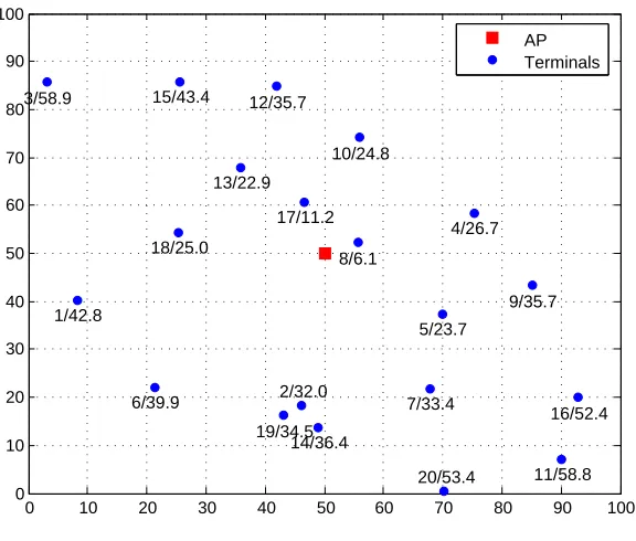
2.1 An example multiple access channel withn = 20nodes communicating with a

common access point (AP). Nodes are randomly placed in a 100 m×100 m square

and the AP is located at the center of the square. Nodes’ labels represent indexes

and distances to the AP. Subsequent numerical experiments use this realization of

the random placement. . . 29

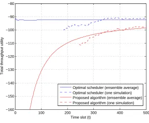
2.2 Convergence of the proposed algorithm to near optimal utility with instantaneous

power constrains but no average power constraints. Throughput utility of the

pro-posed adaptive algorithm and of the optimal offline scheduler are shown as

func-tions of time for one realization and for the ensemble average of realizafunc-tions. In

steady state the adaptive algorithm operates with minimal performance loss with

respect to the optimal offline scheduler. A utility gap smaller than 10 is achieved

in about 350 iterations. Power constraintpinst

i = 100mW, step size= 0.1, capacity

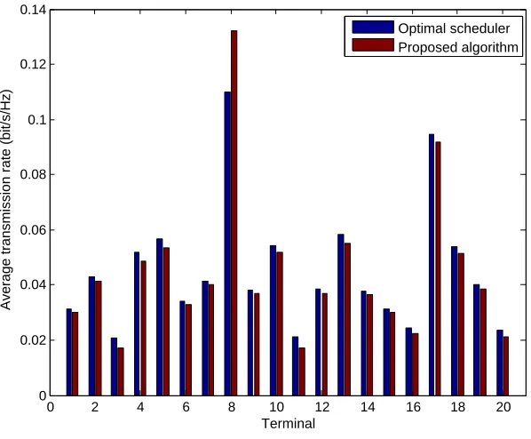
2.3 Average transmission rates (bits/s/Hz) in 500 time slots, i.e.,r¯i(500)as defined in

(2.40), for all terminals. The optimal offline scheduler and the proposed adaptive

algorithm yield similar close to optimal average rates. The variation in achieved

rates is commensurate with the variation in average signal to noise ratios (SNRs)

due to different distances to the access point. For the network in Fig.2.1 and the

pathloss and power parameters used here, average signal to noise ratios vary

be-tween 0.4 and 10. Instantaneous power constraintpinst

i = 100mW, step size= 0.1,

capacity achieving codes. . . 33

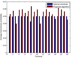
2.4 Average transmission probabilities in 500 time slots for all terminals. Offline and

adaptive optimal schedulers shown. Despite different channel conditions all

ter-minals transmit with a similar probability close to1/n = 0.05. This is consistent

with the use of a logarithmic, i.e., proportional fair, utility. Instantaneous power

constraintpinst

i = 100mW, step size= 0.1, capacity achieving codes. . . 34

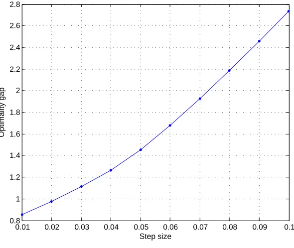
2.5 Steady state optimality gap between proposed adaptive algorithm and optimal

offline scheduler as a function of step size. Values ofbetween10−2_and10−3

shown. As the step size decreases, the optimality gap decreases. The optimality

gap can be made arbitrarily small by reducing. Instantaneous power constraint

pinst

i = 100mW, capacity achieving codes. . . 35

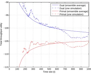
2.6 Primal and dual objectives when instantaneous and average power constraints

are in effect. One realization and ensemble average of realizations shown. As

time grows the duality gap decreases, eventually approaching a small positive

constant and implying near optimality of the achieved rates. Instantaneous power

constraintpinst

i = 100mW, average power constraintp

avg

i = 5mW, step size= 0.1,

adaptive modulation and coding withM = 4modes with ratesτ1= 1bits/s/Hz,

τ2= 2bits/s/Hz,τ3= 3bits/s/Hz, andτ4= 4bits/s/Hz and transitions at SNRs

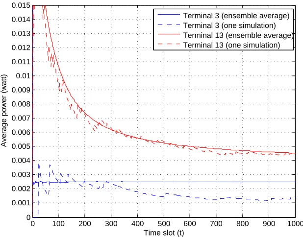
2.7 Average power consumption for terminals 3 and 13, i.e.,p¯3(t)andp¯13(t)as defined

in (2.41). Average power constraints pavg_i = 5mW are satisfied as time grows. Powerp¯3(t)consumed by Terminal 3 is smaller than the allowed budgetpavg3 due

to unfavorable channel conditions. Terminal 13 adheres to its power budget after

approximately 600 iterations. Parameters as in Fig. 2.6 . . . 37

2.8 Instantaneous power allocationspi(t)for terminalsi= 3andi= 13plotted against

the channel realizationhi(t). Notice that the channel axes scales are different in (a)

and (b). In both cases, no power is allocated when channel realizations are bad.

Terminal 3 uses only the AMC mode with the lowest rateτ1= 1bits/s/Hz, while

Terminal 13 uses two modes with ratesτ2 = 2bits/s/Hz andτ3 = 3bits/s/Hz.

This happens because Terminal 13, being closer to the AP, has a better average

channel than Terminal 3. Parameters as in Fig. 2.6. . . 38

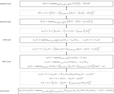
3.1 Layers and layer interfaces. The stochastic subgradient descent algorithm in terms

of layers and layer interfaces. Layers maintain primal variablesak

i(t),rkij(t),˜cij(t),

pij(t),qij(t)as well as auxiliary variablespi(t),xij(t), andyi(t)while multipliers

λk

i(t), µij(t), νij(t),αij(t), βi(t) andξi(t)are associated with interfaces between

adjacent layers. Primal variables can be easily computed based on multipliers

from interfaces to adjacent layers and dual variables are updated using

informa-tion from adjacent layers. . . 51

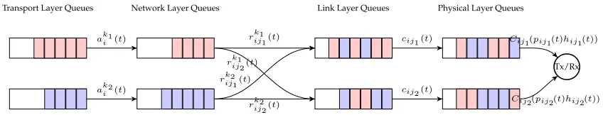
3.2 Queue dynamics. Terminal i operates by controlling queues in different layers

based on operating pointsak

i(t),rijk(t),cij(t),pij(t)andqij(t). In the transport layer

and the network layer, each flowkhas a queue. In the link layer and the physical

layer, each outgoing link(i, j)maintains a queue. In this particular example, there

are two flowsk1andk2 and there are two neighboring nodesj1andj2. Packets

3.3 Message passing. (a) Terminalibegins by transmitting dual variablesλk i(t)and

νij(t)to all neighbors j ∈ N(i). (b) It then computes and shares Pk∈N(i)νki(t)

with allj ∈ N(i). This information, along with locally available multipliers, is

then used to perform the primal iterations associated with all the layers in Fig.3.1.

(c) Terminalipasses primal variablesyi(t)andrijk(t)to all neighborsj∈ N(i). (d)

It then evaluates and broadcastsPk∈N(i)yk(t)toj ∈ N(i). Dual updates

associ-ated with the layer interfaces in Fig.3.1 are now performed using these and locally

accessible primal variables. We proceed to (a) for the next iteration. . . 54

3.4 Connectivity graph of a network with n = 15 terminals randomly placed in a

square with side L = 100meters. Terminals can communicate with neighbors

whose distances are within 30 meters. The numbers on each edge shows the

dis-tance (in meters) between two communicating terminals. . . 67

3.5 Feasibility. After about 500 steps, all constraints are satisfied in an ergodic sense

within 10−2 _{tolerance. The average rate constraint takes the longest time to be}

satisfied. This is because the transmission rate on linkTi →Tj depends not only

on schedules and powers ofTi but also on those ofTj and neighbors ofTj. This

requires information to be received from, and propagated to, 2-hop neighbors. . . 69

3.6 (a) Optimality. As time grows, primal and dual objectives approach each other.

(b) Correlation between Q1(t)and Q6(t). At the beginning, there is significant

correlation betweenQ1(t)andQ6(t). But as time grows, the correlation vanishes

and becomes negligible. . . 70

4.1 Optimal power allocation functionP∗_{(ˆh)(left) and channel backoff functionB}∗_(ˆh)

(right) for single user point-to-point channel. Curves shown for channel state

in-formation (CSI) varianceσ2

e = 0.1,σ2e = 0.1, andσ2e = 0, corresponding to perfect

CSI. As CSI variance increases power allocation is more conservative for small

channel values. When the CSI variance is large, the backoff function selects codes

of a higher rate than what is dictated by the channel estimate. Channel coefficient

follows a complex Gaussian distributionCN(0,2), average power budgetP0= 1,

and channel conditional pdfm_h|ˆhas in (4.9). . . 109

4.2 Convergence of average transmission rate (left) and average power consumption

(right) for Algorithm 2. Average transmission rate as a function of time is shown

for Algorithm 2 and cases in which only the backoff function is optimized –

mean-ing p(t) = P0 – or only the power allocation function is optimized – implying

b(t) = ˆh(t). Joint optimization yields substantial increase of average

communica-tion rate. Average power budgetP0= 1, constant step size= 0.01, and channel

estimation errorσ2

e = 0.1. . . 111

4.3 Rate (left) and power (right) convergence of Algorithm 3. Sum of average

trans-mission rates is shown for Algorithm 3 and two suboptimal solutions. One case

uses a backoff function with fixed outage probability 0.01 and the other case

op-timizes power allocation only – implyingbf

n(t) = ˆhfn(t). Joint optimization yields

substantial increase of average communication rate. Average power budgetP0 =

4, constant step size= 0.01, and channel estimation errorσ2

4.4 Rate (left) and power (right) convergence of Algorithm 4. Proportional fair

util-ity of average transmission rates is shown for Algorithm 4 and two suboptimal

solutions in which only the backoff function – meaningpn(t) = P0,n – or only

the power allocation function – implying bn(t) = ˆhn(t) – are optimized. Joint

optimization yields substantial increase of average communication rate. Average

power budgetP0,n= 1(right), constant step size= 0.01, and channel estimation

errorσ2

e = 0.1. . . 113

5.1 Comparison of the expected sum rate utility achieved by the optimal FDMA (ρ=

1), the optimal RA (ρ = 0) and the proposed algorithm (ρ ∈ {0,0.1,0.2,· · ·,1}).

The total number of terminals isn= 10. . . 141

5.2 The expected sum rate utility achieved by the proposed algorithm normalized by

that achieved by the optimal FDMA forn= 10andn= 50. The horizontal line is

1/e≈0.368. . . 142

5.3 The expected sum rate utility achieved by the proposed algorithm for differentρ.

For all cases, the expected utility increases as the total number of terminals grows. 143

5.4 Comparison of the average sum rate utility of the network achieved by the optimal

FDMA (ρ= 1), the RA (ρ= 0) and the proposed algorithm (ρ∈ {0,0.1,0.2,· · ·,1}).

Chapter 1

Introduction

Optimal design is emerging as the future paradigm for wireless networking. The fundamental

idea is to select operating points as solutions of optimization problems, which, inasmuch as

opti-mization criteria are properly chosen, yield the best possible network. Results in this field include

architectural insights, e.g., [9], and protocol design, e.g., [13, 22], but a drawback shared by most

of these works is that they rely on global channel state information (CSI); i.e., the optimal

vari-ables of a terminal depend on the channels between all pairs of terminals in the network. While

availability of global CSI is plausible in certain situations, it is unlikely to hold if time varying

fading channels are taken into account. In this case, distributed algorithms in which terminals

operate based on locally available CSI are more practical. The focus of this thesis is to develop

distributed algorithms for the optimal design of wireless networks.

When only local CSI is available, operating variables of each terminal are selected as functions

of local CSI. This further leads to the selection of random access as the natural medium access

choice. Indeed, if transmission decisions depend on local channels only and these channels are

random and independent for different terminals, transmission decisions can be viewed as

ran-dom and resultant link capacities as limited by collisions. In this chapter, we present an overview

1.1

Background

1.1.1

Random access wireless channels

Consider a multiple access channel withnterminals contending to communicate with a common

AP. Time is divided in slots identified by an indext. We assume a backlogged system, i.e., all

ter-minals always have packets to transmit in each time slot. The time-varying nonnegative channel

hi(t) ∈R+ between terminaliand the AP at timetis modeled as block fading – for this to be

true the length of a time slot has to be comparable to the coherence time of the channel. Channel

gainshi(t1)andhi(t2)of terminaliat different time slotst1 6=t2are assumed independent and

identically distributed (i.i.d.) with pdfmhi(·). Channel gainshi(t)andhj(t)of different terminals

i6=jare also assumed independent. Channels are assumed to have continuous pdf. This latter

assumption holds true for models used in practice, e.g., Rayleigh, Rician and Nakagami [14, Ch.

3]. We assume each terminal i has access to its channel gain hi(t) at each time slot t. While

there are various alternatives to obtain channel state information, the simplest would be for the

AP to send a beacon signal at the beginning of each time slot. This beacon signal would serve

the double purpose of providing a reference for channel estimation as well as a synchronization

signal.

Based on its channel statehi(t), nodeidecides whether to transmit or not in time slot tby

determining the value of a scheduling functionqi(t) := Qi(hi(t)) : R+ → {0,1}. Nodei

trans-mits in time slot tif qi(t) = 1 and remains silent ifqi(t) = 0. Notice that each terminal has a

different scheduling function and that schedulesqi(t)are determined based on the CSI of each

node independently of other terminals. Although each node has access to its local CSIhi(t), the

underlying pdfmhi(·)is unknown.

Besides channel access decisions, terminals also adapt transmission power to their channel

gains through a power control functionPi(hi(t)) :R+ →[0, pinsti ], wherepinsti ∈R+is a constant

adjusts its transmission powerPi(hi(t))in response tohi(t). Similar toqi(t), we definepi(t) :=

Pi(hi(t)), representing the power allocated to nodeiin time slott. If nodeitransmits in time

slott,pi(t)andhi(t)jointly determine the transmission rate through a functionCi(hi(t)pi(t)) :

R+ →R+. The exact form ofCi(hi(t)pi(t))depends on how the signal is modulated and coded

at the physical layer. Examples considered later in the thesis include capacity-achieving codes

and adaptive modulation and coding (AMC). With capacity-achieving codes,Ci(hi(t)pi(t))takes

the form

Ci(hi(t)pi(t)) =Blog

1 + hi(t)pi(t)

BN0

, (1.1)

whereBandN0are the channel bandwidth and the power spectral density of the channel noise,

respectively. With AMC, there areM transmission modes available. Themth mode affords

com-munication rateτmand is used when the signal to noise ratio (SNR)hi(t)pi(t)/BN0is between

ηmandηm+1. The rate function is therefore

Ci(hi(t)pi(t)) = M

X

m=1

τmI

ηm≤

hi(t)pi(t)

BN0

≤ηm+1

, (1.2)

whereI(·)denotes the indicator function. To keep the analysis general we do not restrict

Ci(hi(t)pi(t))to take either specific form. It is only assumed thatCi(hi(t)pi(t))is a nonnegative

increasing function of the product ofhi(t)andpi(t)that takes finite values for finite arguments.

These assumptions are satisfied by (1.1) and (1.2) and are likely to hold in practice.

Since terminals contend for channel access, transmission of terminaliin a time slottis

suc-cessful if and only ifqi(t) = 1and qj(t) = 0for all j 6= i. If the transmission of terminali is

successful, its transmission rate is determined byCi(hi(t)pi(t)). As as consequence, the

instanta-neous transmission rate for terminaliin time slottis

ri(t) =Ci(hi(t)pi(t))qi(t) n

Y

j=1,j6=i

[1−qj(t)]. (1.3)

be-havior ofri(t). This implies that system performance is determined by the ergodic limits

ri:= lim t→∞

1

t

t

X

u=1

ri(u)

= lim

t→∞

1

t

t

X

u=1



Ci(hi(u)pi(u))qi(u) n

Y

j=1,j6=i

[1−qj(u)]



. (1.4)

Assuming ergodicity of schedulesqi(t) = qi(hi(t))and power allocationspi(t) = pi(hi(t)), the

limitrican be written as a expected value over channel realizations,

ri=Eh



Qi(hi)Ci(hiPi(hi)) n

Y

j=1,j6=i

[1−Qj(hj)]



, (1.5)

where we have defined the vectorh = [h1,· · ·, hn]T grouping all channelshi. An important

observation here is that since terminals are required to make channel access and power control

decisions independently of each other,Qi(hi)andPi(hi)are independent ofQj(hj)andPj(hj)

for alli6=j. This allows us to rewriterias

ri=Ehi[Qi(hi)Ci(hiPi(hi))]

n

Y

j=1,j6=i

1−Ehj[Qj(hj)]

. (1.6)

In addition to instantaneous power constraintspi(t)≤pinsti , terminals adhere to average power

constraintspavgi ∈R+as in, e.g., [8]. This average power constraint restricts the long term average

of transmitted power that we either write as an ergodic limit or as an expectation over channel

realizations,

pi:= lim t→∞

1

t

t

X

u=1

qi(u)pi(u) =Ehi[Qi(hi)Pi(hi)]. (1.7)

1.1.2

Random access wireless networks

Consider an ad-hoc wireless network consisting ofJ terminals indexed asi= 1, . . . J. Network

connectivity is modeled as a graphG= (V,E)with verticesv∈ V :={1, . . . , J}representing theJ

terminals and edgese= (i, j)∈ Econnecting pairs of terminals that can communicate with each

other. Denote the neighborhood of terminaliasN(i) :={j|(i, j)∈ E}and define the interference

can interfere with a transmission fromi toj. The network supports a setK := {1, . . . , K} of

end-to-end flows through multihop transmission. The average rate at whichk-flow packets are

generated atiis denoted byak

i. Terminalitransmits these packets to neighboring terminals at

average ratesrk

ij and, consequently, receivesk-flow packets from neighbors at average ratesrjik.

To conserve flow, exogenous ratesak

i and endogenous ratesrkijat terminalimust satisfy

aki ≤

X

j∈N(i)

rkij−rjik

, for alli∈ V, andk∈ K. (1.8)

Further denote the capacity of the link fromi →j ascij. Since packets of different flowskare

transmitted fromitojat ratesrk

ij it must be

X

k∈K

rkij ≤cij, for all(i, j)∈ E. (1.9)

Unlike wireline networks wherecij are fixed, link capacities in wireless networks are dynamic.

Similar to what we did in Section 1.1.1, let time be divided into slots indexed by tand denote

the channel betweeniandjat timetashij(t). The channel is assumed to be block fading and

channel gainshij(t)of link(i, j)are assumed independent and identically distributed with

prob-ability distribution function (pdf)mhij(·). For reference, define the vector of terminalioutgoing

channels hi(t) := {hij(t)|j ∈ N(i)}and the vector of all channels h(t) := {hij(t)|(i, j) ∈ E}.

Denote their pdfs asmhi(·)andmh(·), respectively.

Based on the channel statehi(t)of his outgoing links, terminalidecides whether to transmit

or not on link(i, j)in time slot t by determining the value of a scheduling functionqij(t) :=

Qij(hi(t))∈ {0,1}. Ifqij(t) = 1, terminalitransmits on link(i, j)and remains silent otherwise.

Further defineqi(t) :=Qi(hi(t)) :=P_j∈N(i)Qij(hi(t))to indicate a transmission fromito any of

his neighbors. We restrictito communicate with, at most, one neighbor per time slot implying

that we must haveqi(t)∈ {0,1}. We emphasize thatqij(t) :=Qij(hi(t))depends on local

outgo-ing channels only and not on global CSI. Further note that terminals have access to instantaneous

local CSIhi(t)but underlying pdfsmhi(·)are unknown.

a power control functionpij(t) := Pij(hi(t))taking values in[0, pinstij ]. Here,pinstij represents the

maximum allowable instantaneous power on link(i, j). The average power consumed by

termi-naliis then given as the expected value over channel realizations of the sum ofPij(hi)over all

j ∈ N(i), i.e.,

pi≥Ehi 

 X

j∈N(i)

Pij(hi)Qij(hi)



, (1.10)

where we also relaxed the equality constraint to an inequality, which can be done without loss

of optimality. If terminal i transmits to node j in time slott, pij(t)and hij(t)determine the

transmission rate through a function Cij(hij(t)pij(t))whose form depends on modulation and

coding.

Due to contention, a transmission fromitojat timetsucceeds if a collision does not occur.

In turn, this happens if: (i) Terminali transmits toj, i.e., qij(t) = 1. (ii) Terminalj is silent,

i.e.,qj(t) = 0. (iii) No other neighbor ofj transmits, i.e. ql(t) = 0for alll ∈ N(j)andl 6= i.

Recalling the definition of interference neighborhoodMi(j)and that if a transmission occurs its

rate isCij(hij(t)pij(t))we express the instantaneous transmission rate fromitoj in time slott

ascij(t) :=cij(hi(t)) =Cij(hij(t)pij(t))qij(t)Ql∈Mi(j)[1−ql(t)]. Assuming an ergodic mode of

operation, the capacity of linki→jcan then be written as

cij=Eh



Cij(hijPij(hi))Qij(hi)

Y

l∈Mi(j)

[1−Ql(hl)]



. (1.11)

Because terminals are required to make channel access and power control decisions

indepen-dently of each other, Qij(hi)andPij(hi)are independent ofQlm(hl)andPlm(hl)for alli 6= l.

SinceQl(hl) :=Pm∈N(l)Qlm(hl(t))by definition, it follows thatQij(hi)is also independent of

Ql(hl)for alli6=l. This allows us to write the expectation of the product on the right hand side

of (1.11) as a product of expectations,

cij ≤Ehi

Cij

hijPij(hi)

Qij(hi)

Y

l∈Mi(j)

1−Ehl

Ql(hl)

where we also relaxed the equality constraint to an inequality, which can be done without loss of

optimality1.

The operating point of a wireless network is characterized by variables ak

i, rijk,cij, pi and

functions Pij(hi), Qij(hi). Besides (1.8)-(1.12), these variables are subject to certain box

con-straints. Admission variables, have lower and upper bounds due to application layer

require-ments, i.e.,amin

i ≤ aki ≤amaxi . Similarly, routing variables, link capacities, and terminal power

budgets cannot be negative and are also subject to given upper bounds, i.e., 0 ≤ rk

ij ≤ rijmax,

0 ≤ cij ≤ cmaxij , and0 ≤pi ≤ pmaxi . Furthermore, according to definition, Pij(hi)andQij(hi)

can only take values from[0, pinst

ij ]and{0,1}, respectively. For notational simplicity, we define

vectorsxi :=

pi, akij, rkij, cij :∀j ∈ N(i) andPi(hi) := {Pij(hi), Qij(hi) :∀j∈ N(i)}to group

all the variables related to terminaliand summarize these box constraints as{xi,Pi(hi)} ∈ Bi

with

Bi:=

 

xi,Pi(hi)

amini ≤aki ≤aimax, 0≤rkij ≤rijmax,

0≤cij ≤cmaxij , 0≤pi≤pmaxi , 0≤Pij(hi)≤pinstij ,

Qij(hi)∈ {0,1}, Qi(hi)∈ {0,1}

 

. (1.13)

1.2

Roadmap

Our first investigation focuses on random access channel where terminals contend for

commu-nicating with a the central AP. This models the physical layer of the wireless random access

network we shall study later on. We develop adaptive scheduling and power control algorithms

for random access in a multiple access channel where terminals acquire instantaneous channel

1_{If we have channel reciprocityh}

ij(t) =hji(t), the derivation of (1.12) from (1.11) is no longer valid since power

control and channel access functions of neighboring nodes will have common arguments implying thatQij(hi)and

Qji(hj)would not be independent. The general methodology used here seems applicable but is beyond the scope of the

state information but do not know the probability distribution of the channel [16]. In each time

slot, terminals measure the channel to the common access point. Based on the observed

chan-nel value, they determine whether to transmit or not and, if they decide to do so, adjust their

transmitted power. We show that the proposed algorithm almost surely maximizes a

propor-tional fair utility while adhering to instantaneous and average power constraints. These results

are presented in Chapter 2.

We then generalize the algorithm proposed for random access channel to wireless multihop

networks where each node determines its operating point using its local CSI distributedly [17].

Since the associated optimization problem is neither convex nor amenable to distributed

imple-mentation, a problem approximation is introduced. This approximation is still not convex but it

has zero duality gap and can be solved and decomposed into local subproblems in the dual

do-main. The solution method is through a stochastic subgradient descent algorithm that operates

without knowledge of the fading’s probability distribution and leads to an architecture

com-posed of layers and layer interfaces. With limited amount of message passing among terminals

and small computational cost, we show that the proposed algorithm converges almost surely in

an ergodic sense. These results are presented in Chapter 3.

Both above proposed algorithms require terminals to adapt transmission parameters such as

power and rate to time-varying channel conditions to improve system’s overall performance.

Al-though accurate CSI is essential to achieve this goal, perfect CSI is rarely available in practice due

to estimation errors and, perhaps more fundamentally, to feedback delay. Our next topic is to

de-velop algorithms to handle imperfect CSI in the transmission over wireless channels [18]. In

par-ticular, we consider three types of wireless channels, namely single user point-to-point block

fad-ing channels [15], multiuser downlink orthogonal frequency division multiplexfad-ing (OFDM) [38],

and multiuser uplink random access (RA) [29], where the transmitter adapt transmitted power

and coding mode to imperfect channel estimates in order to maximize expected throughput

between channel estimates and actual channel values, a backoff function is further introduced to

enforce the selection of more conservative coding modes. Joint determination of optimal power

allocations and backoff functions is a nonconvex stochastic optimization problem with infinitely

many variables that despite its lack of convexity is part of a class of problems with null duality

gap. Exploiting the resulting equivalence between primal and dual problems, we show that

op-timal power allocations and channel backoff functions are uniquely determined by opop-timal dual

variables. This affords considerable simplification because the dual problem is convex and finite

dimensional. We further exploit this reduction in computational complexity to develop iterative

algorithms to find optimal operating points. These results are presented in Chapter 4.

So far the distributed algorithms we developed are based on local CSI only (either perfect

or imperfect). In practice, terminals may have knowledge about channels of neighboring nodes

in addition to local CSI. This motivates us to investigate wireless networks where each terminal

has a different belief about the global channel states and adapts its transmission policy to the

belief. In this setting, frequency division multiple access (FDMA) and channel aware random

access (RA) are two special cases where perfect global and local CSI are available, respectively.

To find solutions for general cases, we formulate the problem as a Bayesian game in which each

terminal maximizes the expected utility based on its belief. We show that optimal solutions for

both FDMA and RA are equilibrium points of the game. Therefore, the proposed game theoretic

formulation can be regarded as general framework for multiuser wireless communications.

Fur-thermore, we develop a cognitive access algorithm that solves the problem approximately. These

Chapter 2

Distributed algorithms for optimal

random access channels

In this chapter, we consider wireless random access channels in which terminals contend for

ac-cess to a common acac-cess point (AP) as introduced in Section 1.1.1. To exploit favorable channel

conditions terminals adapt their transmitted power and access decisions to the state of the

ran-dom fading channels linking them to the AP. The challenges in developing this adaptive scheme

are that terminals have access to their own channel state information (CSI) only, and that the

probability distribution function (pdf) of the fading channel is unknown. Our goal is to develop

a distributed learning algorithm to determine optimal transmitted power and channel access

decisions relying on local CSI only.

The idea of adapting medium access and power control to CSI has been extensively explored

in wireless communications. Early references dealing with power adaptation on the uplink of

multiuser systems focus on centralized power control schemes where the AP collects channel

states for all terminals to select the one to be scheduled. In, e.g., [19], the AP schedules the

have also been used for scheduling and resource allocation in broadcast downlink channels, see

e.g., [3, 11, 23]. Although these centralized schemes exploit multiuser diversity, they require

sig-nificant information exchange between terminals and the AP; a problem exacerbated when the

number of users is large. To avoid this overhead, recent work integrates channel adaptation into

random access protocols. Exploiting the idea of aligning schedules to good channel

opportuni-ties, [29] develops a distributed channel-aware Aloha protocol in which terminals transmit only

when their channel gains exceed pre-defined thresholds. This algorithm is shown to be

asymp-totically optimal in the sense that the only performance loss compared to a centralized scheme is

due to user contention.

Under simple collision models, it has been shown that distributed threshold-based schedulers

with properly designed thresholds maximize total throughput of a network with homogeneous

users and total logarithmic throughput in the case of heterogeneous users [50]. Similar

threshold-based decentralized adaptive random access schemes have been investigated for other types of

networks with different packet reception models, see e.g., [1, 6, 25, 27, 30, 46, 51]. To compute

the optimal thresholds, however, terminals are assumed to know the probability distribution of

their fading channels. This is a restrictive assumption because the channel fading distribution is

usually unknown and can only be estimated based on channel observations. Overcoming this

limitation motivates the development of adaptive algorithms to learn optimal operating points

based on local CSI [4, 37]. The work in [4] proposes a heuristic adaptive algorithm for

threshold-based schedulers in which the thresholds are tuned threshold-based on local channel realizations in a time

window. The work in [37] develops an online learning algorithm for transmission probability

and power control under rate constraints using game-theoretic approaches. However, neither [4]

nor [37] guarantees global optimality.

The contribution of this chapter is the development of an optimal distributed adaptive

algo-rithm for scheduling and power control given that terminals only have access to local CSI and

and decide whether to transmit or not. If they decide to transmit, they choose a power for their

communication attempt. As time progresses, power budgets are satisfied almost surely, while the

network almost surely maximizes a weighted proportional fair utility. We remark that terminals

operate independently without access to the channel state of other terminals and that the channel

pdf is unknown. The proposed algorithm can handle general non-convex, even discontinuous,

rate functions with manageable computational complexity. It is worth noting that under the

frame work of network utility maximization (NUM) algorithms for computing optimal channel

access probabilities in random access networks are developed (see e.g. [21]). However, neither

fading nor power adaptation is considered in these work.

The presentation begins by formulating optimal adaptive random access as a utility

max-imization problem whose objective is to maximize a weighted sum of throughput logarithms

(Section 2.1). The variables to be determined as a solution of this optimization problem are a

scheduling function that determines if a terminal should transmit or not based on its CSI, and

a power allocation function that maps a terminal CSI to its transmit power. It is important to

remark that: (i) because fading takes on a continuum of values, this optimization problem is

infinite-dimensional; (ii) the constraints modeling random access are non-convex; (iii) despite

the existence of these non-convex constraints optimization problems of this form are known to

have null duality gap [33]; and (iv) since the number of constraints turns out to be finite the

op-timization problem is finite-dimensional in the dual domain. A further complication is that the

original problem formulation yields solutions that require access to global CSI.

We start by overcoming the dependence on global CSI by introducing an equivalent

decompo-sition in per-terminal subproblems whereby nodes maximize local utilities (Section 2.2.A). While

this reformulation yields solutions that depend on local CSI only, attempting a solution in the

primal domain is difficult because the per-terminal subproblems inherit infinite dimensionality

and lack of convexity from the original problem formulation, as well as the need to have access to

a stochastic subgradient descent algorithm in the dual domain (Section 2.2.B). Based on channel

realizations in each time slot, the algorithm computes instantaneous values for the scheduling

and power allocation functions and updates Lagrangian multipliers in a direction that can be

proven to point towards the set of optimal dual variables in an average sense (Proposition 1).

Exploiting this fact we prove that the throughput utility achieved by the algorithm almost surely

converges to a value close to the optimal utility. The gap between the optimal and the achieved

utility can be made arbitrarily small by reducing a fixed step size (Theorem 1). The chapter closes

with a numerical evaluation of the proposed algorithm for a randomly generated heterogeneous

network (Section 2.3). To illustrate generality of the proposed approach we consider a system

with terminals employing capacity achieving codes (Section 2.3.1) and a more practical scenario

with nodes employing adaptive modulation and coding (Section 2.3.2). Concluding remarks are

presented in Section 2.4.

2.1

Problem formulation

Consider a random access channel as introduced in Section 1.1.1. With ratesri given as in (1.6),

our objective is to maximize a weighted proportional fair (WPF) utility defined as

U(r) =

n

X

i=1

wilog(ri), (2.1)

wherer= [r1,· · · , rn]T is the vector of rates andwi∈R+is the weight coefficient for terminali.

Settingwi=wjfor alli6=jin a homogenous system with all channels having the same pdf, the

WPF utility is equivalent to maximizing the sum of throughputs. In a heterogeneous network

where channel pdfs vary among users, maximizing U(r) yields solutions that are fair since it

prevents users from having very low transmission rates.

access is formulated as the following optimization problem

P = max U(r)

s.t. ri=Ehi[Qi(hi)Ci(hiPi(hi))]

n

Y

j=1,j6=i

1−_Ehj[Qj(hj)]

,

Ehi[Qi(hi)Pi(hi)]≤p

avg

i ,

Qi(hi)∈ Q, Pi(hi)∈ Pi,∀i (2.2)

whereQis the set of functionsR+ → {0,1}taking values on{0,1}andPirepresents the set of

functionsR+→[0, pinst

i ]taking values on[0, pinsti ]. Notice that the joint optimization across users

required to solve (2.2) introducesfunctionaldependence between the actions of different

termi-nals. This is not incongruent with the requirement ofstatisticallyindependent schedules in each

time slot. In fact, the notationsQi(hi)andPi(hi)in (2.2) stipulates that terminals are required

to make channel access and power allocation decisions based on local CSI only. Consequently,

although problem (9) requires joint optimization across users, it restricts optimization to policies

that result in statistically independent operations.

The goal of this chapter is to develop an online algorithm to determine schedulesqi(t)and

power assignments pi(t)having statistics that solve the optimization problem in (2.2). The

al-gorithm is required to: (i) operate without knowledge of the channel distribution; and (ii) yield

functionsqi(t)andpi(t)that depend on the current and past values of the local channelhi(t)but

are independent of other terminal’s channelshj(t)forj6=i.

Remark 1. In order to allow terminals to know if their transmissions are successful or not, the AP provides feedback on whether the transmission attempt was successful or a collision detected. If a terminal transmits

a packet but detects a collision, it can reschedule the packet for retransmission in a subsequent time slot.

We remark that feedback does not introduce correlation between the transmission decisions of different

terminals. The provided feedback only tells terminals if they should retransmit previous packets or not, but

2.2

Adaptive algorithms for optimal random access channels

The stated goal is to devise scheduling and power control policies based on local CSI that are

globally optimal as per (2.2). These two objectives, i.e., global optimality while relying on local

CSI, seem to contradict each other. Becauseri depends not only onQi(hi)and Pi(hi)but on

Qj(hj)for allj 6=i, it seems that optimalQi(hi)andPi(hi)solving (2.2) might also be functions

of other terminals’ CSI. To see that this is not the case, we will show that it is possible to

decom-pose (2.2) in per terminal subproblems. After introducing this decomposition the complicating

fact that the channel pdf fhi(hi)is unknown remains. To overcome this complication, we will

introduce a stochastic subgradient descent algorithm in the dual domain that is optimal in an

ergodic sense.

2.2.1

Problem decomposition and its dual

Begin then by separating (2.2) in per terminal subproblems. To do so, we substitute (1.6) into

(2.1) and express the logarithm of a product as a sum of logarithms. As a result, the global utility

in (2.1) can be rewritten as

U(r) =

n

X

i=1

wi



logEhi[Qi(hi)Ci(hiPi(hi))] +

n

X

j=1,j6=i

log1−Ehj[Qj(hj)] _

. (2.3)

Note that each summand in (2.3) only involves variables related to a particular node. Thus, we

can reorder summands in (2.3) to group all of the terms pertaining to nodei. Further defining

˜

wi:=Pn_j=1,j6=iwi, we can rewrite (2.3) as

U(r) =

n

X

i=1

wilog [Ehi[Qi(hi)Ci(hiPi(hi))]] + ˜wilog [1−Ehi[Qi(hi)]]

:=

n

X

i=1

Ui, (2.4)

where we have defined the local utilities Ui. SinceUi only involves variables that are related

to terminal i, it can be regarded as a utility function for terminali. To maximizeU(r)for the

whole system it suffices to separately maximize Ui for each terminal i. Introducing auxiliary

the following per terminal subproblems

Pi = maxwilogxi+ ˜wilog(1−yi)

s.t. xi≤Ehi[Qi(hi)Ci(hiPi(hi))],

yi≥Ehi[Qi(hi)],

Ehi[Qi(hi)Pi(hi)]≤p

avg

i ,

xi≥0,0≤yi≤1, Qi(hi)∈ Q, Pi(hi)∈ Pi, (2.5)

where we relaxed the equality constraints to inequality ones which can be done without loss of

optimality. Finding optimal solutions of (2.5) for all terminalsi is equivalent to solving (2.2).

Different from (2.2), however, there is no coupling between variables of different terminals in

(2.5). This property leads naturally to optimalQi(hi)andPi(hi)that are independent of other

terminals’ CSI as required by problem definition. Alas, (2.5) inherits the complex structure of

(2.2).

As is the case with (2.2), solving (2.5) is difficult because: (i) The optimization space in (2.5)

includes functionsQi(hi)andPi(hi)that are defined onR+, implying that the dimension of the

problem is infinite. (ii) The rate functionCi(hiPi(hi))is in general non-concave with respect to

hiPi(hi), and may be even discontinuous as in (1.2). (iii) The constraints involve expected values

over random variableshiwhose pdfs are unknown.

An important observation is that the number of constraints in (2.5) is finite. This implies that

while there are infinite variables in the primal domain, there are a finite number of variables

in the dual domain. This observation suggests that (2.5) is more tractable in the dual space.

Introduce then Lagrange multipliersλi= [λi1, λi2, λi3]T associated with the first three inequality

constraints in (2.5); define vectorsxi := [xi, yi]T andPi(hi) := [Qi(hi), Pi(hi)]T; and write the

Lagragian of the optimization problem in (2.5) as

+λi2[yi−Ehi[Qi(hi)]] +λi3

pavg_i −_Ehi[Qi(hi)Pi(hi)]

=λi3pavgi + [wilogxi−λi1xi] + [ ˜wilog(1−yi) +λi2yi]

+Ehi[Qi(hi) [λi1Ci(hiPi(hi))−λi2−λi3Pi(hi)]]. (2.6)

where the second equality follows after reordering terms in the first equation. Notice that the

first term in the second equality in (2.6) depends onxionly, the second term onyiand the third

term onPi(hi)andQi(hi). This property is exploited later on. The dual function is then defined

as the maximum of the Lagrangian over the set of feasiblexiandPi(hi), i.e.,

gi(λi) := max Li(xi,Pi(hi),λi)

s.t. xi≥0,0≤yi≤1, Qi(hi)∈ Q, Pi(hi)∈ Pi. (2.7)

We now can write the dual problem as the minimum ofgi(λi)over positive dual variables, i.e.,

Di = min

λi≥0

gi(λi). (2.8)

In general, the optimal dual valueDi of (2.8) provides an upper bound for the optimal primal

valuePi of (2.5), i.e.,Di ≥ Pi. While the inequality is typically strict for non-convex problems,

for the problem in (2.5)Pi=Dias long as the fading distribution has no realization with positive

probability [33]. Notice that this is true despite the non-convex constraints present in (2.5). This

lack of duality gap implies that the finite dimensional convex dual problem is equivalent to the

infinite dimensional nonconvex primal problem. While this affords a substantial improvement

in computational tractability, it does not necessarily mean that solving the dual problem is easy

because evaluation of the dual function’s value requires maximization of the Lagrangian. In

particular, this maximization includes an expected value over the unknown channel distribution

fhi(hi). Still, convexity of the dual function allows the use of descent algorithms in the dual

domain because any local optimal solution is a global optimal solutionλ∗_i = [λ∗

i1, λ∗i2, λ∗i3]T. This

property is exploited next to develop a stochastic subgradient descent algorithm that solves (2.8)

2.2.2

Adaptive algorithms using stochastic subgradient descent

Instead of directly finding optimal xi, yi, Qi(hi)and Pi(hi) for the primal problem (2.5), the

proposed algorithm exploits the lack of duality gap to use a stochastic subgradient descent in the

dual domain. Starting from given dual variablesλi(t), the algorithm computes instantaneous

primal variablesxi(t),yi(t),qi(t)andpi(t)based on channel realizationhi(t)in time slott, and

uses these values to update dual variables λi(t+ 1). Specifically, the algorithm starts finding

primal variables that optimize the summands of the Lagrangian in (2.6) (the operator[·]+_denotes

projection in the positive orthant)

xi(t) = argmax xi≥0

{wilogxi−λi1(t)xi}=

wi

λi1(t)

, (2.9)

yi(t) = argmax

0≤yi≤1

{w˜ilog(1−yi) +λi2(t)yi}=

1− w˜i λi2(t)

+

, (2.10)

{qi(t), pi(t)}= argmax qi∈{0,1},pi∈[0,pinsti ]

{qi[λi1(t)Ci(hi(t)pi)−λi2(t)−λi3(t)pi]}, (2.11)

The maximization in (2.11) determines schedules and transmitted power associated with current

channel realizationhi(t). Sinceqi in (2.11) takes values on{0,1}the objective is either0when

qi = 0orλi1(t)Ci(hi(t)pi)−λi2(t)−λi3(t)piwhenqi = 1. Thus, to solve (2.11) we only need to

find the optimalpi(t)whenqi(t) = 1and see if the resulting objective is greater than 0. Thus, we

can rewrite (2.11) as

pi(t) = argmax pi∈[0,pinsti ]

{λi1(t)Ci(hi(t)pi)−λi2(t)−λi3(t)pi},

qi(t) =H

λi1(t)Ci(hi(t)pi(t))−λi2(t)−λi3(t)pi(t)

, (2.12)

whereH(a)denotes Heaviside’s step function withH(a) = 1fora >0andH(a) = 0otherwise.

Based onxi(t),yi(t),qi(t)andpi(t), define the stochastic subgradientsi(t)= [si1(t), si2(t),si3(t)]T

with components

si1(t) =qi(t)Ci(hi(t)pi(t))−xi(t), (2.13)

si3(t) =pavgi −qi(t)pi(t). (2.15)

The algorithm is completed with the introduction of a constant step sizeand a descent update

in the dual domain along the stochastic subgradientsi(t)

λil(t+ 1) = [λil(t)−sil(t)]+, forl= 1,2,3. (2.16)

Notice that computation of variables in (2.9)-(2.16) does not require information exchanges

be-tween terminals. This guaranteesQi(hi)andPi(hi)to be independent ofQj(hj)andPj(hj)for all

i6=jas required by problem formulation. The proposed algorithm is summarized in Algorithm

1.

To analyze convergence of (2.9)-(2.16) let us start by showing thatsi(t)is indeed a stochastic

subgradient of the dual function as stated in the following proposition.

Proposition 1. Givenλi(t), the expected value of the stochastic subgradientsi(t)is a subgradient of the

dual function in(2.7), i.e.,∀λi≥0,

Ehi

sT_i(t)|λi(t)(λi(t)−λi)≥gi(λi(t))−gi(λi). (2.17)

In particular,

Ehi

sT_i(t)|λi(t)(λi(t)−λ∗i)≥gi(λi(t))−Di≥0. (2.18)

Proof. See Appendix 2.5.1.

Proposition 1 states that the average of the stochastic subgradient si(t) is a subgradient of

the dual function. We can then think of an alternative algorithm by replacingEhi

si(t)

λi(t)

for

si(t)in the dual iteration step (2.16), which would amount to a subgradient descent algorithm for

the dual function. Since,Ehi

si(t)

λi(t)

points towardsλ∗– the angle betweenEhi

si(t)

λi(t)

andλi(t)−λ∗i is positive as indicated by (2.18) –, it is not difficult to prove thatλi(t)eventually

approachesλ∗_i, e.g., [39, Ch. 2]. However, since we assume the pdf ofhiis unknown, the

subgra-dientEhi

si(t)

λi(t)

can only be approximated using past channel realizationshi(1), . . . , hi(t).

Algorithm 1:Adaptive scheduling and power control at terminali

1 Initialize Lagrangian multipliersλi(0);

2 fort= 0,1,2,· · · do

3 Compute primal variables as per (2.9), (2.10), and (2.12):

4 xi(t) =

wi

λi1(t);

5 yi(t) =

1− w˜i λi2(t)

+

;

6 pi(t) = argmax

pi∈[0,pinsti ]

{λi1(t)Ci(hi(t)pi)−λi2(t)−λi3(t)pi};

7 qi(t) =H

λi1(t)Ci(hi(t)pi(t))−λi2(t)−λi3(t)pi(t)

;

8 ifqi(t) = 1then

9 Transmit with powerpi(t);

10 end

11 Compute stochastic subgradients as per (2.13)-(2.15):

12 si1(t) =qi(t)Ci(hi(t)pi(t))−xi(t);

13 si2(t) =yi(t)−qi(t);

14 si3(t) =pavgi −qi(t)pi(t);

15 Update dual variables as per (2.16):

16 λil(t+ 1) = [λil(t)−sil(t)]+, forl= 1,2,3;

The computation of the stochastic subgradientsi(t), on the contrary, is simple because it only

depends on the current channel statehi(t). Furthermore, since si(t)points towards the set of

optimal dual variables λ∗_i on average [cf. (2.18)] it is reasonable to expect the stochastic sub-gradient descent iterations in (2.16) to also approachλ∗_i in some sense. This can be proved true and leveraged to prove almost sure convergence of primal iteratesxi(t),yi(t),pi(t)andqi(t)to

an optimal operating point in an ergodic sense [31]. Specifically, Theorem 1 of [31] assumes as

hypotheses that the second moment of the norm of the stochastic subgradientsi(t)is finite, i.e.,

Ehi

ksi(t)k2

λi(t)

≤Sˆ2

i, and that there exists a set of strictly feasible primal variables that

sat-isfy the constraints in (2.5) with strict inequality. If these hypotheses are true, primal iterates

of dual stochastic subgradient descent are almost surely feasible in an ergodic sense. For the

particular case of the problem in (2.5), [31, Theorem 1] implies that

lim t→∞ 1 t t X u=1

qi(u)pi(u)≤pavgi a.s., (2.19)

lim t→∞ 1 t t X u=1

xi(u)≤ lim t→∞ 1 t t X u=1

qi(u)Ci(hi(u)pi(u)) a.s., (2.20)

lim t→∞ 1 t t X u=1

yi(u)≥ lim t→∞ 1 t t X u=1

qi(u) a.s. (2.21)

It also follows from [31, Theorem 1] thatxi(t)and yi(t)yield ergodic utilities that are almost

surely withinSˆ2

i/2of optimal, i.e.,

Pi− lim

t→∞ 1 t t X u=1

[wilogxi(u) + ˜wilog(1−yi(u))]≤

Sˆ2

i

2 a.s. (2.22)

From (2.19) we can conclude that the ergodic limit of the power allocated by the proposed

algo-rithm satisfies the average power constraint. However, (2.22) does not imply that the scheduling

and power allocation variablespi(t)andqi(t)are optimal. The optimality claim in (2.22) is for the

auxiliary variablesxi(t)andyi(t)but the goal here is to claim optimality of the scheduling and

power allocation variablespi(t)andqi(t). To prove optimality of the algorithm, we need to show

that the ergodic transmission rateriof (1.4), achieved by allocationsqi(t)andpi(t)is optimal in

If the constraints in (2.5) were satisfied for all timest, i.e., if xi(t) ≤ qi(t)Ci(hi(t)pi(t))and

yi(t)≥qi(t), transforming (2.22) into an almost sure near optimality claim for the ergodic limit

riis a simple matter of substitution and algebraic manipulation. However, these inequalities do

not necessarily hold for all timest. They hold in an ergodic sense as stated in (2.20) and (2.21).

This subtle yet fundamental mismatch is addressed in the proof of the following theorem.

Theorem 1. Consider a random multiple access channel with n terminals using schedulesqi(t) and

power allocations pi(t) generated by the algorithm defined by (2.9)-(2.16) resulting in instantaneous

transmission rates ri(t)as given by(1.3)and ergodic rates ri as defined by (1.4). Define vectorr :=

[r1, . . . , rn]T, and letU(r)be the weighted proportional fair utility in(2.1). Assume that the second

mo-ment of the norm of the stochastic subgradientsi(t)with components as in(2.13)-(2.15)is finite1, i.e.,

Ehi

ksi(t)k2

λi(t)

≤Sˆ2

i, and that there exists a set of strictly feasible primal variables that satisfy the

constraints in(2.5)with strict inequality. Then, the average power constraint is almost surely satisfied

lim

t→∞

1

t

t

X

u=1

qi(u)pi(u)≤pavgi a.s., (2.23)

and the utility of the ergodic limit of the transmission rates almost surely converges to a value within

/2Pn_i=1Sˆ2

i of optimality,

P−U(r) :=P−

n

X

i=1

wilog lim t→∞

1

t

t

X

u=1

ri(u)

! ≤

2

n

X

i=1 ˆ

Si2. (2.24)

Proof. The hypotheses of Theorem 1 are chosen to satisfy the hypotheses guaranteeing

conver-gence of ergodic stochastic optimization algorithms [31, Theorem 1]. Thus, almost sure feasibility

and almost sure near optimality of iteratesxi(t),yi(t),pi(t)andqi(t)follows in the sense of

(2.19)-(2.22). To establish almost sure satisfaction of average power constraints as per (2.23) just notice

that this inequality coincides with the one in (2.19). To establish (2.24) start by rearranging terms

in (2.22) to conclude thatPi−Sˆi2/2 ≤limt→∞1t

Pt

u=1[wilogxi(u) + ˜wilog(1−yi(u))]. Due to

1_{The finite assumption of the second moment of the subgradients is necessary for the proof of almost sure near}

continuity and concavity of the logarithm function we can further boundPi−Sˆi2/2as

Pi−

Sˆ2

i

2 ≤wilog

" lim t→∞ 1 t t X u=1

xi(u)

#

+ ˜wilog

"

1− lim

t→∞ 1 t t X u=1

yi(u)

#

. (2.25)

The limits in (2.25) are equal to the limits in the left hand sides of the inequalities in (2.20) and

(2.21). Thus, using this almost sure ergodic feasibility resultsPi−Sˆi2/2is bounded as

Pi−

Sˆ2

i

2 ≤wilog

" lim t→∞ 1 t t X u=1

qi(u)Ci(hi(u)pi(u))

#

+ ˜wilog

"

1− lim

t→∞ 1 t t X u=1

qi(u)

#

. (2.26)

Ergodicity, possibly restricted to an ergodic component, allows replacement of the ergodic limits

in (2.27) by the corresponding expected values, leading to the bound

Pi−

Sˆ2

i

2 ≤wilogEhi[Qi(hi)Ci(hiPi(hi))] + ˜wilogEhi[1−Qi(hi)]. (2.27)

Recall thatP=Pn_i=1Pi per definition, and consider the sum of the inequalities in (2.27) for all

terminalsiso as to write

P−

n

X

i=1

Sˆ2

i

2 ≤

n

X

i=1

wilogEhi[Qi(hi)Ci(hiPi(hi))] + ˜wilogEhi[1−Qi(hi)] ≤

n

X

i=1

wilog



Ehi[Qi(hi)Ci(hi(t)Pi(hi))]

n

Y

j=1,j6=i

Ehj[1−Qj(hj)] 

, (2.28)

where the second inequality follows by using the definitionw˜i:=Pnj=1,j6=iwi, reordering terms

in the sum, and rewriting a sum of logarithms as the logarithm of a product.

The fundamental observation in this proof is that the scheduling functionQi(hi)and the

power allocation functionPi(hi)are independent of the correspondingQj(hj)andPj(hj)of other

terminals. This is not a coincidence, but the intended goal of reformulating (2.2) as (2.5). Using

this independence, the product of expectations in (2.28) can be written as single expectation over

the vector channelhto yield

P−

n

X

i=1

Sˆ2

i

2 ≤

n

X

i=1

wilog

 Eh



Qi(hi)Ci(hiPi(hi)) n

Y

j=1,j6=i

(1−Qj(hj))

  

. (2.29)

expectation in (2.29) by an ergodic limit to yield

P−

n

X

i=1

Sˆ2

i

2 ≤

n

X

i=1

wilog

 lim

t→∞

1

t

t

X

u=1

qi(u)Ci(hi(u)pi(u)) n

Y

j=1,j6=i

(1−qj(u))



:=U(r), (2.30)

where we have used the definitions of the ergodic rate in (1.4) and of the utility in (2.1). The result

in (2.24) follows after reordering terms in (2.30).

Theorem 1 states that the stochastic dual descent algorithm in (2.9)-(2.16) computes

sched-ulesqi(t)and power allocationspi(t)yielding ratesri(t)that are almost surely near optimal in

an ergodic sense [cf. (2.24)]. It also states thatpi(t)satisfies the average power constraint with

probability 1. Notice that the stochastic dual descent algorithm in (2.9)-(2.16) does not compute

the optimal scheduling and power control functions for each terminal. Rather, it draws schedules

qi(t)and power allocationspi(t)that are close to the optimal functions. This is not a drawback

because the latter property is sufficient for a practical implementation. Further note that the use

of constant step sizesendows the algorithm with adaptability to time-varying channel

distri-butions. This is important in practice because wireless channels are non-stationary due to user

mobility and environmental dynamics. The gap between U(r)and Pcan be made arbitrarily

small by reducing.

Remark 2. The desired optimal schedulesQ∗_{(h(t))and power allocationsP}∗_{(h(t))as prescribed in} Sec-tion 2.1 are funcSec-tions of the current channel realizaSec-tions only. The proposed online policy, however,

com-putes schedulesqi(t)and power allocationspi(t)based on the current channelhi(t)and dual variables

λi(t). In each time slot the iterative policy updatesλi(t)usingλi(t−1)and stochastic subgradientssi(t)

which depend onqi(t),pi(t)andhi(t). As a result, the dual variableλi(t)depends on all previous

chan-nel gains fromhi(0)up tohi(t). Sinceqi(t)andpi(t)are functions ofλi(t), they depend on all previous

channel gains as well. This is not a contradiction because as the algorithm progresses,λi(t)approaches

the optimal multiplierλ∗_i, implying that the time-dependent variablesqi(t), pi(t)converge towards the

optimal policyP∗_{(h(t)), Q}∗_{(h(t)). As a matter of fact,λ}

i(t)does not converge toλ∗i, but to a

algorithm’s (arbitrarily small) optimality penalty as stated in Theorem 1.

2.2.3

Structure of the optimal primal solution

While the algorithm in (2.9)-(2.16) provides a method to find the optimal operating point for the

random multiple access channel, it does not provide intuition on the properties of this operating

point. This section studies structural properties of the optimal primal solution.

In convex optimization problems optimal primal variables are obtained as the Lagrangian

maximizers for optimal dual variables. The optimization problem in (2.5) is not convex. This

is not a hindrance because the recovery of optimal primals from optimal duals through

La-grangian maximization follows from the lack of duality gap, which is a property that (2.5) does

possess [33]. Let us then begin by showing that the optimal primal variablesx∗_i = [x∗

i, y∗i]T and

P∗_i(hi) = [Q∗i(hi), Pi∗(hi)]T of the primal problem in (2.5) can be obtained from the maximizers

of the LagrangianLi(xi,Pi(hi),λ∗i). From the definition of the dual function in (2.7), the optimal

dual value can be written as

Di=gi(λ∗i) = maxLi(xi,Pi(hi),λ∗i) (2.31)

s.t. xi ≥0,0≤yi≤1, Qi(hi)∈ Q, Pi(hi)∈ Pi.

Since the maximization in (2.31) is with respect to all primal variables satisfying the stated

con-straints and the optimal variablesx∗_i andP∗_i(hi)satisfy these constraints, it must be

Di≥ Li(x∗i,P∗i(hi),λ∗i). (2.32)

Consider now the explicit expression ofLi(x∗i,P∗i(hi),λ∗i)as it follows from the definition in (2.6)

Li(x∗i,P∗i(hi),λ∗i) = wilogx∗i + ˜wilog(1−y∗i) +λ∗i1[Ehi[Q ∗

i(hi)Ci(hiPi∗(hi))]−x∗i]

+λ∗i2[yi∗−Ehi[Q ∗

i(hi)]] +λ∗i3

pavg_i −_Ehi[Q ∗

i(hi)Pi∗(hi)]. (2.33)

Sincex∗_i andP∗_i(hi)are solutions of (2.5), they are feasible, i.e., they satisfy the inequalities in

(2.5). Thus, the terms Ehi[Q∗i(hi)Ci(hiPi∗(hi))]−x∗i ≥ 0, yi∗ −Ehi[Q∗i(hi)] ≥ 0, and p

avg