IMPROVEMENT AND COMPARISON OF THREE META HEURISTICS TO OPTIMIZE FLEXIBLE FLOW-SHOP SCHEDULING PROBLEMS

IMPROVEMENT AND COMPARISON OF

THREE META HEURISTICS TO

OPTIMIZE FLEXIBLE FLOW-SHOP

SCHEDULING PROBLEMS

Wahyudin P. Syam

1. Department of Industrial Engineering, King Saud University, Riyadh, 11421, Kingdom of Saudi Arabia 2. Princess Fatimah Alnijris’s Research Chair for Advance Manufacturing Technology

([email protected])

Ibrahim M. Al-Harkan

Department of Industrial Engineering, King Saud University, Riyadh, 11421, Kingdom of Saudi Arabia ([email protected])

Abstract

This study improved and comprehensively compared three Meta heuristics to minimize make-span (Cmax) for Flexible Flow-Shop (FFC) Scheduling Problem. This problem is known to be NP-Hard. This study proposed an improvement for three Meta heuristic searches which are Genetic Algorithm (GA), Simulated Annealing (SA), and Tabu Search (TS). SA and TS are known as deterministic improvement heuristic search. Meanwhile, GA is known as stochastic improvement heuristic search. In addition, in this paper, the three Meta heuristic searches were compared to the GA developed by Kahraman et al. by using a computational analysis. The results for the experiments conducted show that the improved Meta heuristics are better and the TS is the most effective and efficient algorithm to solve FFC scheduling problems.

Keywords: Scheduling, Heuristics, Genetic algorithms, Simulated annealing, Tabu search.

1. Introduction

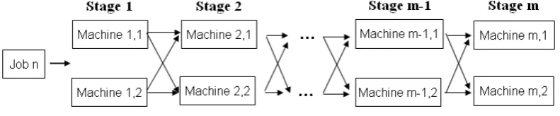
Scheduling is allocating limited resources (machine, gate, people, etc) to certain task to optimize objective functions (Lee, et al. 1997). Flexible Flow Shop (FFC) is one kind of scheduling problem. FFC is a combination of Parallel machine and Flow shop scheduling (Pinedo, 2008; Ronconi and Henriques, 2009; Nowicki and Smutnicki, 1998). In addition, it is a generalization of flow shop problem (Brah and Loo, 1999). In FFC, jobs are processed through some stages, in any stage m, there are two or more identical machine i that can process the job. Fig. 1 shows FFC scheme. The job in each stage will be processed by every machine that is idle. The machines have capacity constraint so that only one job machine can process at a time.

The notation for this scheduling problem is as follows: FFC | perm | Cmax (Pinedo, 2008). The meaning of this notation is as follows: Flexible flow shop scheduling environment with all jobs have identical sequence, queues may or may not follow First come First Served (FCFS), and to minimize make-span.

According to Hong Wang (1998), Mathematical model for FFC is as follows:

Notation of the FFC model:

J: The set of the job to be scheduled |J| = N: number of jobs

s: Number of stages that all jobs will be processed with the same order.

j: Subscript letter representing job j.

l: Subscript letter representing stage l.

i: Subscript letter representing machine i.

:

l

m

Number of identical parallel machine in stage l.

B: A very large positive number.

:

jl

S

Starting time of job j in stage l. ,

, ,

,l s j j J l ∈ ∀ ∈

∀ m .., ... 1, i J, j j, s, l l, otherwise 0 l. stage at i machine on is j job if 1, Xjli = ∈ ∀ ∈ ∀    = m .., ... 1, i J, j j, s, l l, otherwise 0 l stage on i machine on g job before is f job if 1, Y_fgli = ∈ ∀ ∈ ∀    =

:

lj

p

Processing time of job j at stage l.

J, j j, s, l

l, ∈ ∀ ∈

∀ Objective Function: Minimize Q Subject to: j Q; p

Sjs+ js ≤ ∀ (1)

s l l j S p

S_jl + _jl ≤ _j,l+1;∀,, ≠ (2)

g f g f i l Y B S p

S_{fl fl gl fgli}

≠ ∀ − + ≤ + , , , , ); 1 ( (3)

g

f

g

f

i

l

Y

Y

fgli gfli

≠

∀

≤

+

,

,

,

,

;

1

(4) g f g f i l Y Y X

Xfli gli fgli gfli

≠ ∀ + + ≤ + , , , , ; 1 (5)



= ∀ = ml i

jli j l

X

1

, ;

1 (6)

l j

S_jl≥0; ∀, (7)

} 1 . 0 { , _fgli ∈ jli Y

X (8)

Explanation of the model are as follows: (1) indicates that Q is the completion time of the last job j at the last stage s. (2) indicates that it is impossible for every job j to be processed at stage l+1 before every job j is completed at stage l, (3), (4), and (5) are the processing order for jobs f and g on machine i at stage l. These constraints are defined to guarantee that one machine can only process one job at any time, (6) guarantee that one job can only be processed on one machine at any time, (7) provides non-negativity constraint for variable S, (8) restricts that the value of X and Y only have 0 or 1.

To solve FFC problem, we presented three improvement heuristic searches (Lee, at al. 1997), which are Genetic

solve identical problem instances to directly compare performance of these three searches algorithm. The problems to be solved consist of small size problem to big size problem that are considerable NP-hard to be analytically solved. By using these searches, the problem can be solved in polynomial time computation. From the experiment result, performances of these three searches are studied.

The structures of this paper are organized as follows. In section 2, description of improvement heuristic search, as one kind of heuristic search, will be presented. Detail of improvement heuristic search, which are GA, SA, and TS will be presented in section 3, 4, and 5 respectively. Experiment result will be presented in section 6 and closed by conclusion in section 7.

2. Improvement Heuristic Search

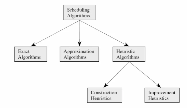
In scheduling problem, there are three classifications of search algorithms, which are exact algorithms, approximation algorithms, and heuristic algorithms as in Fig. 2. Exact algorithm is a complete enumeration search that searches all feasible solution in solution region. This algorithm will give optimum solution. Exact algorithm has limited implementation regarding to computational time for large size problem. Branch and bound is kind of exact algorithm. Approximation algorithm is a search algorithm that uses mathematical formulation to guide the search direction to find good feasible solution. Heuristic algorithm is a search algorithm that uses certain rule to search feasible solution in solution region to find good feasible solution.

Fig. 2 Classification of search algorithm in scheduling problem.

Heuristic search consist of two groups, which are construction heuristic and improvement heuristic (Koulamas, 1998; Ronconi, 2004). Construction heuristic is heuristic search that start from empty schedule solution set and, in each iteration, one job is added into schedule solution set until all jobs are scheduled. Improvement heuristic search is heuristic search that start from initial complete schedule, generated randomly or with certain dispatching rule and the schedule solution set is improved in each iteration until reach certain stopping criteria. GA, SA, and TS are classified as improvement heuristic search.

The background to use approximation search or heuristic search is significantly less computational time even though this search can only give good solution, optimum by chance. Approximation and heuristic search is effective for large scale problem size, especially for problems that are NP-hard if it is solved using exact algorithm.

3. Genetic Algorithm

To generate new population, GA makes selection from current population to choose the best individual in current population and uses operators to create the new population on new generation. The operators are: Crossover and Mutation. By crossover operation, GA generates the neighborhood to explore new feasible solution (Kahraman, et al. 2008; Zhou, et al. 2009; Low and Yeh, 2009; Chou, 2009; Martin, 2009; Al-Harkan, 1997).

3.1 Selection

This process chooses the best individual with fitness function. The fitness function is:



=

=

n

j j i i

f

f

P

1

(9)

3.2 Crossover

Crossover is GA operator to generate new individual to fill the population of the new generation. Parents are randomly chosen from individuals from last generation and selected by crossover rate, that is probability that one individual will become parent. There are many methods for crossover operator (Kellegoz, 2008), which are: Position Based Crossover (PBX), Order Based Crossover (OBX), One Point Crossover (1PX), Cycle Crossover Operator (CX), Order Crossover (OX), Linier Order Crossover (LOX), Partially Mapped Crossover (PMX), Two Point Crossover Version 1 (2PX_V1), Two Point Crossover Version 2 (2PX_V2), and Two Point Crossover Version 3 (2PX_V3).

3.3 Mutation

The objective of mutation operator is to prevent search space fall into local optima. It hopes that by avoiding local optima, it can give near global optima result. Mutation process is an optional process for chromosome. That is why the probability (mutation rate) number is very small. There are two common types of mutations, which are:

3.3.1 Inversion

Inversion mutation as in Fig. 3 is method to randomly change the position of gene with other gene in chromosome.

Fig. 3 Mutation Inversion

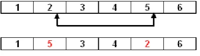
3.3.2 Pair-wise Interchange

Pair-wise interchange as in Fig. 4 is method to change the position between two adjacent genes in chromosome.

Fig. 4 Mutation Pair-wise

Genetic Algorithm Step:

STEP 1: Generate initial population P (0) randomly and Set i=0

STEP 2: REPEAT

P

_i<



=

=

n

j j f f

f

f

P

1

(10)

b. Apply crossover according to crossover rate. c. Apply mutation according to mutation rate.

d. produce offspring or child until the population is filled up. STEP 3: UNTIL Stopping criteria is satisfied.

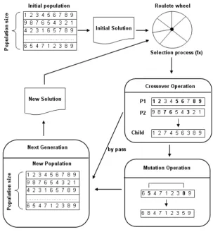
In Fig. 5, scheme of GA is presented. From the scheme, not every new individual, resulted from crossover operation, will be mutated. Only some new individual will be mutated depend on its mutation rate.

Maximum 70% populations of next generation are chosen by roulette wheel method using fitness function (9). The rest of the populations will be filled by crossover operation that is done from crossing two random individuals, according to crossover rate, from populations of the last generation. The crossover processes will be iteratively done until individuals in the next generation reach the population size. Subsequently, mutation operation will be done to some individuals in new generation according to its mutation rate.

4. Simulated Annealing

SA is one of improvement heuristic search. SA is more deterministic compared to GA. SA starts from one initial solution and, in each iteration, new solution will be generated to improve the solution. SA allows accepting bad solution in certain probability, called probability acceptance test. With probability acceptance test, it can avoid local optima while searching around the neighborhood. SA uses interchange operator to generate its neighborhood. There are two most common interchange operators, which are SWAP and Pair-wise Interchange. In GA, these two operators are used to escape from local optima instead of generating neighborhood.

In the beginning, Final, Current, and Candidate have identical initial solution. Then, in each iteration, current solution is compared with Final solution that has been recorded, if current solution is better than the final solution, then current solution will become candidate solution, if it is not, with some probability, this worst current solution can still be acceptable. The process continues until stopping criteria is reached.

Simulated Annealing Algorithm: Let:

Sf = Final Solution found so far. Sc = Candidate Solution. Sk = Solution on Kth Iteration. F(Sf) = Value of Final Solution. F(Sc) = Value of Candidate Solution. F(Sk) = Value of Kth Iteration.

P(F(Sk), F(Sc)) = Probability from moving from Sk schedule to Sc Schedule.

[0,1]

α

and

parameter

cooling

α

β

β

:

where

e

β

F(Sc) F(Sk)

=

=

×

=

−

(11)

STEP 1: Set k = 1 Set β1 and α

Set initial solution S1 Set Sf = S1

Set F(Sf) = F(S1)

STEP 2: Generate K+1 solution (using SWAP or Pair-wise Interchange)

Evaluate F(Sk):

IF F(Sk) < F(Sf) which is better THEN Sc = Sk

Sf = Sk F(Sf) = F(Sk) ELSE

Calculate P(F(Sk), F(Sc)) Generate Random Number U[0,1]

IF U<P(F(Sk),F(Sc)) THEN

Sc = Sk

ELSE

Sk+1 = Sk

STEP 3: Set k = k+1 and β = β x α IF k = N THEN STOP ELSE GOTO STEP 2

5. Tabu Search

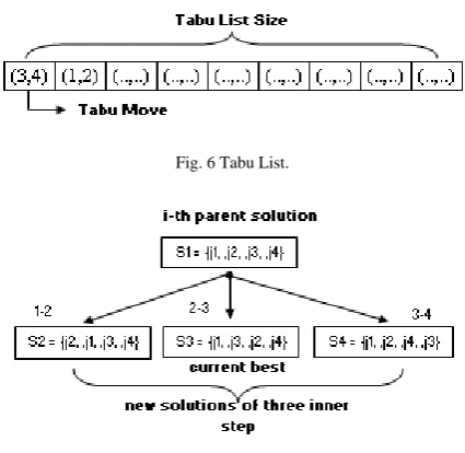
TS has similar characteristic with SA in which that it starts from one initial solution and iteratively generate new solution to search through its neighborhood (Zhou, et al. 2009). In TS, acceptance of moving to other solution in neighborhood is not probabilistic like SA, but deterministic. Records of move, called Tabu move, are kept in a list, called Tabu list as depicted in Fig. 6. The function of Tabu list is to remember moves that have been done, so that it will avoid identical move.

Fig. 6 Tabu List.

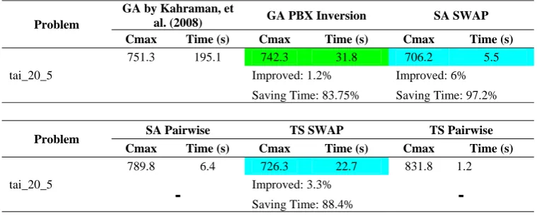
Fig. 7 Example of inner step.

Before generating the neighborhood, TS move will be checked in tabu list. After new solution neighborhoods generated, the best solution on its iteration will be chosen as the parent for the next solutions generation.

Tabu Search Algorithm: STEP 1: Initialization.

Set k = 1

Generate initial solution S0 Set S1 = S0, then G(S1) = G(S0)

STEP 2: Moving.

Select Sc from neighborhood of Sk

IF move from Sk to Sc is already in Tabu list THEN Sk+1 = Sk, GOTO STEP 3

END IF

IF G(Sc) < G(S0) THEN S0 = SC

END IF

Delete the Tabu move in the bottom of Tabu list Add new Tabu Move in the top of Tabu list GOTO STEP 3

STEP 3: Next Iteration. Set k = k + 1 IF k = N THEN STOP

ELSE

GOTO STEP 2

END IF

Kahraman, et al. (2008) used PBX crossover and inversion mutation in their best GA. Subsequently, the improved GA used identical PBX crossover and inversion mutation for comparison. The last two improved SA and TS used SWAP and pair-wise operator.

6. Experiment Results

resulted from 10 GA solutions, 2 SA solutions, and 2 TS solutions. 10’s GA solutions were resulted from 10 different crossover operations. Crossover operator was chosen to differentiate the result because crossover operators are the way GA generated new neighborhood or solutions. Crossover operators that were used: PBX, OBX, 1PX, CX, OX, LOX, PMX, 2PX_V1, 2PX_V2, and 2PX_V3. Pair-wise interchange was used for GA mutation operation. SWAP and pair-wise interchange are neighborhood generation method for SA and TS to obtain different results. Then, total number of runs were 12 Problem sets

×

10 problems instances on each problem set

×

14 different solution approach = 1680 number of runs. Naming system of the problem set were tai_NumberOfJobs_NumberOfStages. i.e. tai_50_20a is FFC problem with 500 jobs, 20 stages, and subtype problem

a. All stages of the problem consist of two identical parallel machines.

Parameters setting for GA were population size = 100, Number of generation = 100, Crossover ratio = 0.9, and Mutation ratio = 0.1. Parameters setting for SA are Cooling parameter = 100,

α

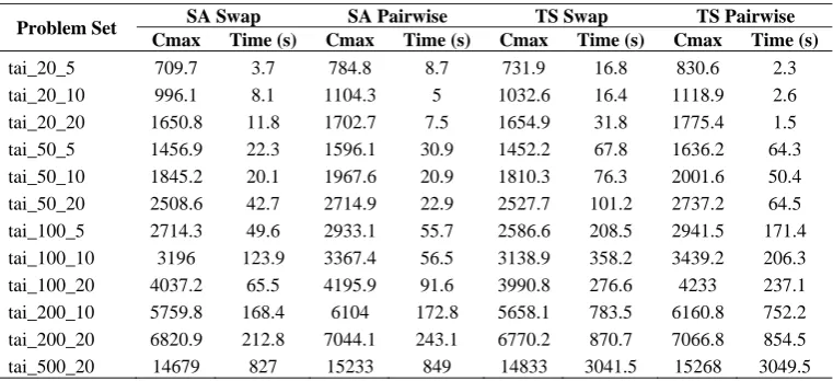
=0.8, and number of iterations = 1000. Parameters setting for TS are Tabu List size = 20, Number of inner steps = 5, and number of iteration = 1000. Computer specifications to run all the computer code to solve the problems were Intel Core 2 Duo 2 GHz, 1GB DDR2 Memory, 80 GB hardisk, and Windows XP SP2 operating system.

These parameters setting of GA, SA, and TS were tested to be compared with the result from reference GA (Kahraman, et al. 2008). This reference GA had the best parameters setting as follows: using PBX crossover with crossover rate = 0.3, using inversion mutation with mutation rate 0.1, population size = 25 and number of generation = 1000. Its selection method used roulette wheel which was generate random number between 1 and total Cmax of all chromosomes and create Cmax slot to determine which chromosome to be selected as parents. In Table 1, it shows that proposed GA, SA, and TS improve the result of reference GA, both for Cmax and computation time. High mutation rate = 0.9 of the proposed GA significantly reduces the computation time compared to reference GA. Results from run of all problem sets are shown in Table 2a, 2b, and 2c. The results were an average result from 10 problems in each problem set. The run results consisted of 14 solutions of average Cmax and average computation time from each problem set.

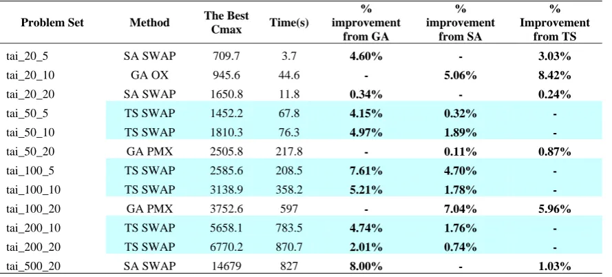
In Table 3, the best solutions of Cmax from each problem set are presented. On each problem set, methods that had the best result are shown as well as result of percentage (%) improvement compared with the other methods. TS produces 6 best results. Meanwhile, both SA and GA produce 3 best results. All the best results of TS and SA are resulted from SWAP neighborhood generation. And, the best results from GA are mostly obtained from OX, PMX, and 2PX_V2 crossover. TS produce most of the best result because it used 5 inner steps to generate neighborhoods in each iteration. It forced TS to widely explore feasible solution space. It increased the probability to find optimal solution. In GA, crossover rate used was 0.9; it means that 90% probability of gene will become parents to create a new population. It transformed feasible solution space, explored by GA, into a narrow space so that it reduced the probability to find optimal solution.

In Fig. 8, comparisons of computation time are shown. SA has the minimum computation time and GA has the maximum computation time. In this experiment, TS computation times are between SA and GA computation times. For SA, computation times only depend on problem size and number of iteration. In the contrary, for GA and TS, computation times are not merely depending on problem size and number of iteration (in GA, number of generation). GA computation time also depends on population size and TS computation time also depends on the number of inner steps applied. From the graph in Fig. 8, TS algorithm is efficient to solve the problem in computation time and effective to solve FFC problems.

Table 1. Improvement results of proposed heuristic search

Problem

GA by Kahraman, et

al. (2008) GA PBX Inversion SA SWAP

Cmax Time (s) Cmax Time (s) Cmax Time (s)

tai_20_5

751.3 195.1 742.3 31.8 706.2 5.5

Improved: 1.2% Improved: 6%

Saving Time: 83.75% Saving Time: 97.2%

Problem SA Pairwise TS SWAP TS Pairwise

Cmax Time (s) Cmax Time (s) Cmax Time (s)

tai_20_5

789.8 6.4 726.3 22.7 831.8 1.2

-

Improved: 3.3%

-

Table 2a. Average Cmax and computational time.

Problem Set GA PBX GA OBX GA CX GA OX GA 1PX

Cmax Time (s) Cmax Time (s) Cmax Time (s) Cmax Time (s) Cmax Time (s)

tai_20_5 744.4 32.2 767.5 34.6 745.2 30.9 746.1 31.3 755.7 31.4

tai_20_10 1046.3 42.6 1069.4 42.7 1040.1 43.6 945.6 44.6 1042.3 41.9

tai_20_20 1656.8 74.5 1682.9 74.8 1659.3 85.8 1656.5 146.9 1660.8 85.4

tai_50_5 1532.4 152.2 1552.4 125.9 1525.8 135.9 1520 134.6 1527.3 137.2

tai_50_10 1918.5 158.7 1953.1 168 1913.1 159 1913.9 161.8 1914.4 175.7

tai_50_20 2515.5 225.6 2647.6 297.8 2606 210.7 2605.8 210.6 2617.6 347.8

tai_100_5 2802.7 490.9 2854.4 493.8 2801.2 456.9 2799.7 651.4 2808.6 574.4

tai_100_10 3324.6 550.2 3360 543 3304.3 544 3312.6 571.7 3309.3 735.7

tai_100_20 4123.8 594.4 4170.7 626.7 4116.4 597.1 4113.2 604.2 4127.6 591.4

tai_200_10 5962.8 1573.1 6042.9 1531.6 5952.3 1619.2 5952.6 1587.9 5971.4 1638.6

tai_200_20 6926.3 1814.5 7001.8 1772.5 6922.4 1823.8 6931.2 1840.1 6922.3 1901.6

tai_500_20 15041 9037.5 15134 9107 14986 9107 15024 9117 15033.5 8917

Table 2b. Average Cmax and computational time (continued).

Problem Set GA LOX GA PMX GA 2PX_V1 GA 2PX_V2 GA 2PX_V3

Cmax Time (s) Cmax Time (s) Cmax Time (s) Cmax Time (s) Cmax Time (s)

tai_20_5 751.3 30.8 748.4 37.1 755.7 36.2 750.2 30.6 750.8 34.4

tai_20_10 1042.5 45.4 1047 43.7 1053.9 40.6 1042.1 49.1 1048.3 44.9

tai_20_20 1663.2 173 1662.1 74.6 1684.7 85.5 1663.3 143.1 1661.5 98.7

tai_50_5 1536.7 135.5 1520.3 135.3 1545.4 313.9 1515.1 205.7 1528.9 132.6

tai_50_10 1923.7 172.2 1919.5 180.3 1919.6 191.7 1905.1 171 1917.8 167.7

tai_50_20 2615.3 222.8 2505.8 217.8 2622.2 225.7 2605.7 230.5 2608 209

tai_100_5 2827.3 434.1 2805.1 458.6 2815.3 525.8 2812.8 524 2800.4 541.1

tai_100_10 3326.8 492.8 3314.2 515.3 3315.6 480.9 3314.9 487.8 3307.8 488.9

tai_100_20 4129.2 605.4 3752.6 597 4125.3 631.2 4121.2 631.2 4120.5 607.2

tai_200_10 5996.6 1565.2 5948.8 1871.4 5973.2 1737.4 5940.1 1722.5 5962.6 1777.3

tai_200_20 6922.3 1801.9 6909.6 1748.4 6948.3 1734.1 6944.6 1762.2 6943.6 1766.4

tai_500_20 15063.5 9017 14995 9147.5 15029 9017.5 14988 9013 14957 9023

Table 2c. Average Cmax and computational time (continued).

Problem Set SA Swap SA Pairwise TS Swap TS Pairwise

Cmax Time (s) Cmax Time (s) Cmax Time (s) Cmax Time (s)

tai_20_5 709.7 3.7 784.8 8.7 731.9 16.8 830.6 2.3

tai_20_10 996.1 8.1 1104.3 5 1032.6 16.4 1118.9 2.6

tai_20_20 1650.8 11.8 1702.7 7.5 1654.9 31.8 1775.4 1.5

tai_50_5 1456.9 22.3 1596.1 30.9 1452.2 67.8 1636.2 64.3

tai_50_10 1845.2 20.1 1967.6 20.9 1810.3 76.3 2001.6 50.4

tai_50_20 2508.6 42.7 2714.9 22.9 2527.7 101.2 2737.2 64.5

tai_100_5 2714.3 49.6 2933.1 55.7 2586.6 208.5 2941.5 171.4

tai_100_10 3196 123.9 3367.4 56.5 3138.9 358.2 3439.2 206.3

tai_100_20 4037.2 65.5 4195.9 91.6 3990.8 276.6 4233 237.1 tai_200_10 5759.8 168.4 6104 172.8 5658.1 783.5 6160.8 752.2 tai_200_20 6820.9 212.8 7044.1 243.1 6770.2 870.7 7066.8 854.5

0 100 200 300 400 500 600 700 800 900 1000 1100 1200 1300 1400 1500 1600 1700 1800 1900 2000 2100 2200 2300 2400 2500

0 1 2 3 4 5 6 7 8 9 10 11 12

GA PBX

GA OBX

GA CX

GA OX

GA 1PX

GA LOX

GA PMX GA 2PX_V1

GA 2PX_V2

GA 2PX_V3

SA SWAP

SA Pairwise

TS SWAP

TS Pairwise

GA

TS

SA Time(s)

Tai_20_5 Tai_20_10 Tai_20_50 Tai_50_5 Tai_50_10 Tai_50_20 Tai_100_5 Tai_100_10 Tai_100_20 Tai_200_10 Tai_200_20 Tai_500_20

Problem Type

GA

TS

SA

Table 3. The best result from each problem set.

Problem Set Method The Best

Cmax Time(s)

% improvement

from GA

% improvement

from SA

% Improvement

from TS

tai_20_5 SA SWAP 709.7 3.7 4.60% - 3.03%

tai_20_10 GA OX 945.6 44.6 - 5.06% 8.42%

tai_20_20 SA SWAP 1650.8 11.8 0.34% - 0.24%

tai_50_5 TS SWAP 1452.2 67.8 4.15% 0.32% -

tai_50_10 TS SWAP 1810.3 76.3 4.97% 1.89% -

tai_50_20 GA PMX 2505.8 217.8 - 0.11% 0.87%

tai_100_5 TS SWAP 2585.6 208.5 7.61% 4.70% -

tai_100_10 TS SWAP 3138.9 358.2 5.21% 1.78% -

tai_100_20 GA PMX 3752.6 597 - 7.04% 5.96%

tai_200_10 TS SWAP 5658.1 783.5 4.74% 1.76% -

tai_200_20 TS SWAP 6770.2 870.7 2.01% 0.74% -

tai_500_20 SA SWAP 14679 827 8.00% - 1.03%

7. Conclusion

In this paper, we present three improvement heuristic searches, which are GA, SA, and TS, to solve FFC scheduling

problems that is known to be NP-hard. The problem consisted of two identical parallel machines in each stage. Experiment used problems from Taillard (1993) that have problem size ranging from 20 jobs to 500 jobs. Improvement of three improved heuristic searches show better result for Cmax and computation time compared to

GA by Kahraman, et al. (2008). Subsequently, effectiveness and efficiency comparisons of the three improvement heuristic searches are presented. From the experiment result, TS produces the most effective result with efficient computation time to solve FFC scheduling problems.

References

[1] C. Y. Lee, L. Lei, M. Pinedo, Current Trends in Deterministic Scheduling, Annals of Operations Research. 70 (1997) 1-41. [2] M. L. Pinedo, Scheduling: Theory, Algorithms, and Systems, 3rd _{edn,” (Springer Science and Business Media, New York, 2008).}

[3] D. P. Ronconi and L. R. R. R. Henriques, Some Heuristic Algorithm for Total Tardiness Minimization in a Flowshop with Blocking,

OMEGA The International Journal of Management Science. 37 (2009) 272-281.

[4] E. Nowicki and C. Smutnicki, The Flow Shop with Parallel Machines: A Tabu Search Approach, European Journal of Operational Research.106 (1998) 226-253.

[5] S. A. Brah and L. L. Loo, Heuristic for scheduling in a flow shop with multiple processors, European Journal of Operation Research. 113

(1999) 113-122.

[6] M. A. Hong Wang, A new model in designing neural network in optimization: A Hybrid neural network approach to machine scheduling, (Business Administration Graduate Program, The Ohio State University, Thesis, 1998).

[7] C. Kahraman, O. Engin, I. Kaya, M. K. Yilmaz, An Application of Effective Genetic Algorithm for Solving Hybrid Flowshop Scheduling Problems, International Journal of Computational Intelligence Systems. 1 (2) (2008) 134-147.

[8] C. Koulamas, A New Constructive Heuristic for The Flowshop Scheduling Problem. European Journal of Operational Research. 105

(1998) 66-71.

[9] D. P. Ronconi, A Note on Constructive Heuristic for The Flowshop Problem with Blocking. International Journal of Production Economics,. 87 (2004) 39-48.

[10] H. Zhou, W. Cheung, L. C. Leung, Minimizing Weighted Tardiness of Job-Shop Scheduling using Hybrid Genetic Algorithm. European Journal of Operation Research. 194 (2009) 637-649.

[11] C. Low and Y. Yeh,, Genetic Algorithm-Based Heuristics for An Open Shop Scheduling Problem with Setup, Processing, and Removal Times Separated. Robotics and Computer-Integrated Manufacturing. 25 (2009) 314-322.

[12] F. Chou, An Experienced Learning Genetic Algorithm to Solve The Single Machine Total Weighted Tardiness Scheduling Problem. Expert System with Application. 36 (2009) 3857-3865.

[13] C. H. Martin, A Hybrid Genetic Algorithm / Mathematical Programming Approach to The Multi-Family Flow Shop Scheduling Problem with Lot Streaming. OMEGA: The International Journal of Management Science. 37 (2009) 126-137.

[14] T. Kellegoz, B. Toklu, J. Wilson, Comparing Efficiencies of Genetic Crossover Operators for One Machine Total Weighted Tardiness Problem. Applied Mathematics and Computation.199 (2008) 590-598.

[15] I. M. Al-Harkan, On Merging Sequencing and Scheduling Theory with Genetic Algorithms to Solve Stochastic Job Shops, (Department of Industrial Engineering, University of Oklahoma, PhD Dissertation, 1997).